Low-Order Post-Stall Aerodynamics Modeling for use in Flight Simulation and Stability Analysis.

(1)

ABSTRACT

PAUL, RYAN CHRISTENSEN. Low-Order Post-Stall Aerodynamics Modeling for use in Flight Simulation and Stability Analysis. (Under the direction of Dr. Ashok

Gopalarathnam.)

Aerodynamic models that can be used to rapidly compute forces and moments acting

on a wing or aircraft configuration have applications in flight simulation, design, and flight

dynamics characterization. For use in aerodynamic prediction on arbitrary aircraft

con-figurations, these models are difficult to formulate for situations like post-stall conditions

where flow separation causes the aerodynamics to be highly nonlinear. A decambering

approach, which uses known airfoil section data as input, is studied for incorporation

in an aerodynamics analysis method such as a vortex-lattice formulation. To perform

post-stall aerodynamic analysis of a finite wing, it is necessary to formulate the

decam-bering calculation as a Newton iteration. The application of the Newton iteration to the

decambering problem is non-standard as no closed form expression exists to facilitate the

residual calculation. Four residual calculation methods are evaluated on the basis of

com-putational efficiency and robustness. Solutions for the post-stall behavior of a rectangular

wing using the most appropriate residual calculation method are compared to

computa-tional fluid dynamics predictions. The comparison between the low-order analysis using

decambering and the computational solutions is excellent. With increasing sweep angle,

however, spanwise propagation of separated flow resulting from transverse pressure

gra-dients causes the behavior of wing sections to depart from that of the corresponding

airfoil. This flow phenomenon results in progressively inaccurate prediction with

increas-ing sweep. Next, an architecture is presented for combinincreas-ing the post-stall aerodynamics

(2)

un-steady vortex lattice method. The formulation of the vortex-lattice method in discrete

time is well suited for time marching simulation. Finally, by utilizing a linearized form

of the unsteady vortex lattice equations coupled with a rigid body model the stability of

wings and configurations is studied. The decambering approach lends itself to a natural

incorporation into the stability analysis framework. For post-stall flight dynamics,

de-cambering is introduced into the system matrices by treating it at each strip as a control

effector, whose deflection is linearly related to the change in flight velocities. This

rela-tionship between the change in flight velocities and change in decambering is appended

to the system in feedback form. Results for the post-stall stability analysis are validated

through a study of a free-to-roll wing as compared to experimental results. A full aircraft

configuration is studied to predict the changes in stability characteristics as the post-stall

model is introduced. The trends shown by the rigid body modes as the post-stall effects

are introduced agree well with experiments, but additional study is warranted to validate

(3)

(4)

Low-Order Post-Stall Aerodynamics Modeling for use in Flight Simulation and Stability Analysis

by

Ryan Christensen Paul

A dissertation submitted to the Graduate Faculty of North Carolina State University

in partial fulfillment of the requirements for the Degree of

Doctor of Philosophy

Aerospace Engineering

Raleigh, North Carolina

2015

APPROVED BY:

Dr. Charles Hall Dr. Fen Wu

Dr. Andre Mazzoleni Dr. Ashok Gopalarathnam

(5)

DEDICATION

(6)

BIOGRAPHY

Ryan was born to Chris and Anne Paul in Monterey, California while his dad was

sta-tioned at Fort Ord as part of the Army 7th Infantry Division. Following a move, most of

his childhood was spent between Downingtown, PA and Tulsa, OK, until Tulsa became

a more permanent home for his family in 1993. He graduated Union High School in 2006,

and subsequently attended Oklahoma State University graduating in 2010 with a B.S.

in Aerospace Engineering and a B.S. in Mechanical Engineering. Ryan joined N.C. State

in the Fall of 2010 and shortly thereafter began working with Dr. Goparlarathnam. The

Summer of 2014, Ryan spent working with the Flight Dynamics Branch at NAVAIR,

located in Patuxent River, MD. He looks forward to starting his career at NAVAIR after

(7)

ACKNOWLEDGEMENTS

There are many people to whom I owe gratitude for their guidance and support

through-out my graduate education. First of all, I would have never have pursued grad school

without the excellent instructors during my undergraduate studies at Oklahoma State

University. They instilled in me a desire to learn more, and more importantly, helped me

to develop a work ethic that has since served me well. Dr. Arena at OSU provided me

with opportunities to work on research teams, and these activities were instrumental in

helping me secure the funding that supported the beginnings of my graduate career.

From the beginning of my time at NC State, my research advisor, Dr. Gopalarathnam,

has provided me with constant support and encouragement, without which, this work

would have never been completed. I am grateful for his guidance on research problems

and also for his constant pursuit to make the work we are doing better, even when

a deadline is rapidly approaching. Dr. G is gratefully acknowledged for pushing me to

pursue two opportunities that otherwise may have passed me by. The first occurred when

I was buried deeply in coursework, and he encouraged me to apply to a DoD SMART

Program. Although the application process could not have occurred at a time any less

favorable, it did help establish where I plan to start my career. Secondly, Dr. G worked

to connect our research with Dr. Murua from the University of Surrey which led our

research in different and interesting directions.

Through travel support provided by the UGPN at NC State, I had the opportunity

to spend time working in the UK with Dr. Murua at the University of Surrey. Dr. Murua

is gratefully acknowledged for hosting me in the UK, for providing me with guidance in

the research, and for sharing his SHARP toolset for use in my research.

(8)

coursework, parts of which were implemented into my research work, and for the time

they dedicated to serving on my committee. I also wish to pass my thanks to our wonderful

graduate services coordinator, Annie White, for her help in all administrative matters.

Very generous funding for the first three years of my graduate studies was provided by

the National Science Foundation Graduate Research Fellowship Program. This support is

gratefully acknowledged. Additionally, I am thankful for the DoD SMART Program that

(9)

LIST OF TABLES

Table 3.1 Number of iterations required for convergence for three angles of attack. Under-relaxation factor ofD≤0.6 was needed forα of 24 degrees with scheme A. The numbers in parenthesis for scheme A show the number of iterations required for convergence with D = 0.6 at α of 16 and 30 degrees. Schemes B and C did not converge at the high angles of attack even with damping. Scheme D did not require damping at any

angle of attack. . . 35

Table 4.1 Post-stall example aircraft geometric properties. . . 71

Table 4.2 Post-stall example aircraft mass properties and reference areas. . . 72

Table 5.1 Geometric Properties for the Free-to-Roll Wing . . . 95

Table 5.2 Aircraft geometric properties, inertial properties, and reference infor-mation for the configuration used in the full aircraft used for stability results. . . 103

Table 5.3 Longitudinal continuous-time eigenvalues compared to other analysis method. . . 109

(13)

LIST OF FIGURES

Figure 2.1 Decambering applied to an airfoil: (a) potential- and viscous-flow lift curves (lines) and operating points (symbols) for a cambered airfoil at

α of 2o and 20o; potential-flow lift curves are shown for decambering of δ1 = 0o and −9.65o, (b) airfoil with boundary-layer displacement

thickness forα= 20o _{added, (c) equivalent decambering using a linear}

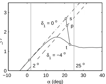
function, and (d) original and modified camberlines. . . 10 Figure 2.2 Geometry of wing-tail configuration used. . . 13 Figure 2.3 Potential-flow operating points for section 5 of the wing are shown

for wing angles of attack of 2o and 25o. Potential-flow lift curves are shown for two values of δ1: 0o (dash-dot line) and −4o (dashed line).

Viscous-flow lift curve for the airfoil is shown as a solid line. For wing

α of 25o are the starting (s) and perturbed (p) operating points which define the trajectory line are shown. The intersection of this line with the viscous lift curve gives the target operating point (t). Vertical lines in gray at α of 2o and 25o are shown for providing context. . . 14 Figure 2.4 Initial section operating points with δ1 = 0 degrees for low and high

values of the wing angle of attack. . . 18

Figure 3.1 Comparison of spanwise Cl distributions from the superposition

ap-proach and direct analysis (using Weissinger method) for wing-tail configuration: (a) Additional loading and two example basic loadings, with the basic loading scaled by 3 times for clarity, (b) Total loading from superposition and direct analysis for α = 10o _{with no}

decam-bering and with δ1 = −3o applied to wing sections 10,11 near the

root. . . 26 Figure 3.2 Comparison of the trajectory lines from the four schemes for section 5

on the wing. The initial operating point (with δ1 = 0 degrees) is for

wing angle of attack of 20 degrees. . . 27 Figure 3.3 Wing-only CL-αcurves from schemes A–D compared with 2D and 3D

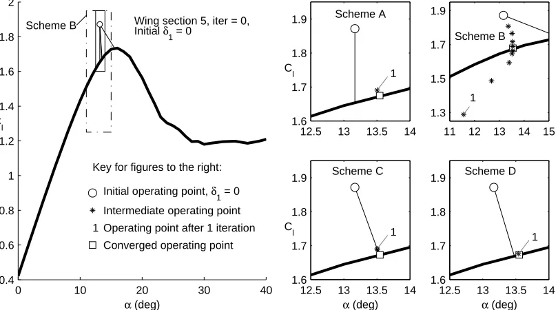
CFD results. . . 33 Figure 3.4 Evolution of the operating points from initial (δ1 = 0 degrees) to

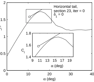
con-verged for section 5 compared for schemes A–D. Wing angle of attack is 16 degrees and no under-relaxation was used with any scheme. . . . 37 Figure 3.5 Trajectory line for section 23 on the tail illustrating the reason for

failure of scheme C. . . 38 Figure 3.6 Effect of initial δ1 value on the evolution of the operating points from

initial (δ1 = 0 degrees) to converged for section 5 for schemes A and

(14)

Figure 3.7 Wing-only lift coefficient vs. angle of attack from schemes D, D0, and D1 compared with 2D and 3D CFD results. Also shows are the results

from one iteration of scheme A. . . 43

Figure 3.8 Comparison of wingCl distributions from schemes D, D0, and D1 with CFD results for α = 14 and 20 degrees. . . 44

Figure 3.9 Comparison of wing Cl distributions using 20 and 80 strips along the wing span, with CFD results for α = 24 and 26 degrees. . . 45

Figure 3.10 Upper-surface flow visualizations on the wing from CFD for 24 and 26 degrees angle of attack. Right side of geometry is shown. . . 45

Figure 3.11 Comparison of wingCl distributions from schemes D, D0, and D1 with CFD results for α = 24 and 26 degrees. . . 47

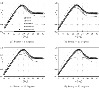
Figure 3.12 Wing-only CL-α curves from schemes D, D0, and D1 compared with CFD for the four aft-sweep angles. . . 49

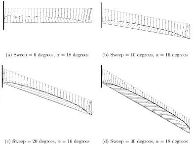
Figure 3.13 Upper-surface flow visualizations on the wings from CFD at CL,max. Right side of each wing is shown. . . 50

Figure 3.14 Comparison of wing Cl distributions for α = 4 and 26 degrees from schemes D, D0, and D1 with CFD results for the four sweep angles. . 51

Figure 4.1 Aerodynamics model showing the lifting-surface and wake discretiza-tion using vortex-ring elements. . . 56

Figure 4.2 Flowchart for the method. . . 62

Figure 4.3 Wing-tail geometry with ring vortices (bound only) shown. The ring vortices corresponding to one spanwise section, or ‘strip’, are high-lighted in blue. . . 65

Figure 4.4 Input viscous data for NACA 0012 airfoil. . . 71

Figure 4.5 Input viscous data for NACA 4415 airfoil. . . 71

Figure 4.6 Post-stall simulation example trajectory. . . 73

Figure 4.7 Elevator command and α response. . . 74

Figure 4.8 Rudder command and β response. . . 74

Figure 4.9 Post-stall Cl distribution at Sim Time = 7.6s. . . 74

Figure 4.10 Unstalled Cl distribution from Sim Time = 20s. . . 74

Figure 5.1 Flowchart describing the process to perform stability analysis cases. . 79

Figure 5.2 Axis system used in the the SHARP Linear Stability Analysis . . . . 81

Figure 5.3 Schematic of the coupling between the linearized aerodynamics and rigid-body systems. . . 84

Figure 5.4 Aircraft undergoing steady roll rate. . . 88

(15)

Figure 5.6 Pole locations corresponding to roll damping plotted as the wing angle of attack is increased. . . 97 Figure 5.7 Operating points for the port wing at various equilibrium

configura-tions for the free to roll wing example. . . 99 Figure 5.8 Variation of non-dimensional roll damping derivative with increase in

the wing angle of attack. . . 100 Figure 5.9 The configuration for the full aircraft stability test case: (a) Isometric

view of the aircraft, and (b) Viscous airfoil input information applied to the main wing. . . 102 Figure 5.10 Trimming routine outline. . . 105 Figure 5.11 Aircraft orientation and operating points for the main wing strips

shown for α = 1 deg. (left) and α= 20 deg. (right). . . 105 Figure 5.12 Trim solutions for 1≤αAC ≤25 degrees. . . 106 Figure 5.13 Variation of the eigenvalues for the longitudinal modes with increase

in angle of attack. . . 108 Figure 5.14 Eigenvalues for the lateral-directional modes plotted as angle of attack

(16)

LIST OF SYMBOLS, ABBREV., NOMENCLATURE

Γb bound circulation vector

Γw wake circulation vector

υ right eigenvector

w non-circulatory velocity vector at collocation points

δ1 decambering variable

γf p flight path angle

λi continuous time eigenvalue

ν body-axis velocities

Θ orientation angles of the body fixed reference frame

ζ aerodynamic lattice coordinate

a0 potential flow lift curve slope

Ab bound aerodynamic influence coefficient matrix

Aw wake aerodynamic influence coefficient matrix

Cl airfoil lift coefficient

Gcon control input matrix

Kb number of bound panels

(17)

Kdec decambering sensitivity matrix

x state vector

z discrete time eigenvalue

(18)

Chapter 1 Introduction

Increasingly, training for flight crews is taking place in simulators rather than actual

aircraft. For effective training to occur, the simulator must accurately replicate the

be-havior of the aircraft. Along with numerous other factors, such as providing realistic

visual effects, control feel, and even motion queues, adequate simulation fidelity requires

that the aerodynamic model be representative of the aircraft. High-fidelity aerodynamic

models implemented in the form of look-up tables are commonplace in certified flight

simulators and training devices. Force and moment information for these look-up tables

is often developed using some combination of the following techniques: computational

fluid dynamics (CFD), experimental testing of models in wind tunnels (static and

dy-namic), and/or experimental flight testing. Developing these data tables requires

signif-icant effort and expense. Each expected operating condition, which is generally defined

by aerodynamic inflow angles, body axis velocities, and other explanatory variables must

be considered using computational analysis, in an experimental environment, or in a

flight test. Assembling the requisite number of test points for a database covering even

(19)

eval-uations, depending on how coarse of a grid between the explanatory variables is deemed

acceptable.

Because of the significant amount of effort and expense required to develop the high

fidelity aerodynamic data, often only a small range of the flight envelope is covered.

Beyond the range of coverage, aerodynamic force and moment data is interpolated (if

possible), held constant, or even extrapolated [1]. As aircraft are not expected to

oper-ate outside the bounds of their aerodynamic model coverage, this approach is normally

acceptable.

However, the need to improve aerodynamic modeling at off nominal operating

con-ditions can not be ignored. In fact, the majority of commercial aircraft accidents, as

reported by Boeing [2] in the years 2004-2013, have been attributed to loss of control.

The general aviation fleet has not fared much better, so much so that the National

Transportation Safety Board has recognized general aviation loss of control in its Most

Wanted improvement areas for 2015 [3]. By definition, loss of control accidents involve

flight outside of the normal aerodynamic operating envelope [4], where the normal

op-erating envelope is characterized by low angle of attack and sideslip excursions. Part of

addressing loss of control as a cause of accidents involves expanding the capability of

aerodynamic models to include high angle of attack regimes [5].

Research performed under the NASA Aviation Safety Program has endeavored, with

admirable success, to expand the modeling capability beyond the nominal flight regime

for transport type configurations. Researchers in this program have proven the capability

of both CFD [6] and carefully designed experiments [7] to represent forces and moments

where significant amounts of flow separation exist, such as aerodynamic stall. While it

may be that the characteristic behaviors discovered in these studies can be modeled and

(20)

applicability to other types of configurations is uncertain.

This research represents a departure from the high-fidelity data-based aerodynamics

modeling being applied to transport configurations discussed above. Rather, a

medium-fidelity aerodynamics analysis method is considered, based on vortex lattice

aerodynam-ics in conjunction with the application of decambering to account for flow separation,

when necessary. This sort of aerodynamics model has the capability to output force and

moment predictions with only geometry and viscous data representing airfoil sections

supplied as input. If formulated properly, the model is well suited to fast aerodynamics

prediction even when being evaluated for post-stall conditions, and has applications in

design, dynamics simulation, and flight dynamics characterization.

1.1 Literature Review

This section provides a brief description of some of past work relevant to the topics in

this document.

1.1.1 Post-Stall Corrections in Potential Flow Aerodynamics

Analysis Methods

For linear conditions such as in pre-stall flight, the ability of low-order linear aerodynamic

methods such as lifting-line theory, Weissinger’s method, and vortex lattice methods

(VLMs) to predict the aerodynamics of multiple lifting surface configurations is well

established. For several decades, researchers have sought to extend these linear prediction

methods to handle the aerodynamic analysis of wings in which nonlinear airfoil lift curves

(21)

The motivation is that it is significantly easier to obtain aerodynamic characteristics for

airfoils than for wings and configurations. The input airfoil data may be generated using

CFD or experiment or by drawing on existing databases from a multitude of sources

— from Abbott and von Doenhoff [20] and those from the University of Stuttgart [21]

and University of Illinois at Urbana-Champaign [[22],[23],[24]], to modern computational

approaches designed to predict sectional aerodynamic characteristics based on arbitrary

input geometry, such as XFOIL [25]. The flow over a wing at post-stall conditions is

highly three dimensional, and the use of a quasi-two-dimensional approach represents a

significant approximation. However, for use in real-time and design-oriented applications,

rapid, albeit approximate approaches that model the important effects of flow separation

on lifting surfaces continue to be of interest.

Efforts at NC State University, initially by Mukherjee and Gopalarathnam [26], led to

the development of a decambering concept which is capable of extending the validity of

a classical VLM or similar to model the effects of separated flow at post-stall conditions.

Research by Cho and Cho [27] has resulted in the incorporation of the decambering

con-cept in a frequency-domain VLM. The post-stall solutions computed using decambering

have shown great promise, and the methodology is further improved as described in this

document.

1.1.2 Aerodynamics in the Loop

An alternative to the use of extensive look-up tables with pre-computed values of

aero-dynamic force and moment coefficients is to use an aeroaero-dynamic calculation method as

the function evaluation to predict forces and moments in a flight dynamics simulation.

(22)

piloted aircraft and the FS One [29] for radio-control aircraft. Both these simulators

use variations of the so-called strip-theory and component-buildup methodologies. In

the strip-theory approach, the lifting surfaces and the bodies are divided into strips.

On each strip at every time step, the forces and moments are determined from the net

velocity at the strip and integrated to get total force and moment on the component.

With component-buildup methodology, aerodynamic forces and moments on different

components of the vehicle are summed up to determine the total force and moment on the

vehicle. Aerodynamic models based on semi-empirical methods are used for determining

the forces and moments on the strips and components. The modeling approach used in

the FS One has been described by Selig in [30]. This paper [30] illustrates the significant

effort and experience necessary to develop efficient semi-empirical aerodynamic models

for use in realistic, full-envelope flight simulation. The development of such semi-empirical

models are often informed by data from myriad sources including wind-tunnel results,

analytical predictions, CFD solutions, flight experiments, and observations of aircraft

flight behavior.

While the approaches described above are able to model the effects of aerodynamic

stall, there are drawbacks to the strip-theory approach besides necessitating empirical

model corrections. The primary disadvantage is in the evaluation of spanwise variations.

Spanwise variations may be modeled correctly using lifting surface methods, such as

vortex lattice models. Vortex lattice aerodynamic models have been combined with the

equations of motion by researchers such as Bunge and Kroo [31], who demonstrated

the use of a VLM formulated in a compact form in real time dynamic simulation, and

Obradovic and Subbarao [32], who used a vortex lattice aerodynamics to model the flight

dynamic behavior of a morphing wing configuration. The aerodynamics in [31] and [32]

(23)

1.1.3 Stability Analysis

Flight dynamics equations are directly obtained by applying the Newton-Euler equations

to the center of gravity of an aircraft. For stability analysis, these nonlinear dynamic

equations are linearized about an equilibrium configuration (corresponding to aircraft

trim) through a Taylor series expansion [33]. In the linearization, the loads generally

are from aerodynamics, weight, and possibly thrust. For a typical aircraft configuration

where it is reasonable to assume that longitudinal and lateral states are decoupled, the

longitudinal stability quartic and lateral stability quintic are obtained, and the modes

may be computed. Stability analysis routines have been implemented using aerodynamic

loads from a vortex lattice method. The linear relationship between the circulations

computed in the VLM and the flight velocities precludes the use of the standard VLM

based stability analysis techniques in situations where flow separation is present.

1.2 Layout of the Document

Chapter 2 begins by describing the decambering approach in two-dimensional flow past

an airfoil. An example calculation for this simple test case is carried out. Next, the

itera-tive process by which the decambering calculation is applied to a finite wing is discussed.

This discussion brings out the principal challenge that must be overcome to perform the

post-stall analysis rapidly, mainly the residual calculation. Four assumptions, leading to

four different residual calculation schemes, and the motivation behind each are presented

in Chapter 3. The residual calculation schemes are compared against one another in

their ability to successfully converge when analyzing a rectangular wing geometry. After

determining the most robust and efficient residual calculation scheme, the

(24)

Chapter 4. Chapter 5 utilizes the toolbox provided by the SHARP routines to study the

flight dynamic characteristics a free-to-roll wing and a full aircraft configuration in the

post-stall regime. Conclusions are drawn in Chapter 6 and recommendations for future

(25)

Chapter 2 The Decambering Post-Stall

Aerodynamic Model

In the following sections, the concept of decambering is explained. The discussion and

figures in this chapter are adapted from Paul and Gopalarathnam [34]. Section 2.1

demon-strates decambering as it is applied first to a two-dimensional airfoil case. For an airfoil

flow, the application of decambering is relatively straightforward, as demonstrated in a

simple example case. Complications arise when decambering is applied to a finite wing.

The interactions between sections that arise when a three-dimensional finite wing is

considered in post-stall analysis cases are described in Section 2.2. Finally, posing the

decambering problem for a finite wing into the framework of a Newton iteration is treated

(26)

2.1 Decambering Applied to a 2D Flow

At small angles of attack, the boundary layer on an airfoil is usually attached and thin. At

these conditions, the predicted lift coefficient from potential-flow methods like thin airfoil

theory agrees excellently with lift coefficient from experiments or viscous computations.

Potential-flow methods do not model any viscous effects. Consequently they predict an

almost linear lift curve having a slope close to 2π per radian, with lift increasing with

angle of attack even beyond stall. As the angle of attack is increased to stall and beyond,

the boundary layer on the upper surface thickens and separates. It is this flow separation

that causes the viscousCl to deviate from the potential-flow theory prediction. Because

the flow separation in effect causes a reduction in camber, the effect is sometimes referred

to in the literature as “viscous decambering” [35] or “decambering.”

The idea behind the current decambering approach is that the potential-flow

predic-tion for lift coefficient of the decambered airfoil at some α will match the viscous Cl at

thatα even if thatα is well beyond the angle of attack for stall. The decambering can be

modeled as an effective reduction in the airfoil angle of attack using a decambering

vari-able δ1 that is given (in radians) by δ1 = (Cl,viscous−Cl,potential)/2π. This is a simplified

version of the two-variable decambering approach described in [26]. Note that camber

reduction due to upper-surface flow separation corresponds to a negative δ1 in this sign

convention.

The overall idea behind decambering is illustrated in Fig. 2.1. Figure 2.1(a)

com-pares the Cl-α curves from potential flow and viscous flow for an airfoil. Considering

two example angles of attack of 2 degrees and 20 degrees, it is seen that the Cl values

from potential flow and viscous flow are nearly identical for the 2-degree case, but are

(27)

−100 0 10 20 30 40 1

2 3

α [deg] C

l

Pot. flow Visc. flow

2o 20o

δ₁ = 0o δ

1 = −9.65 o

(a)

(b)

(c) −9.65

o

0 0.2 0.4 0.6 0.8 1

0 0.05 0.1 0.15 Original Camberline Modified Camberline (d) x/c

Figure 2.1: Decambering applied to an airfoil: (a) potential- and viscous-flow lift curves (lines) and operating points (symbols) for a cambered airfoil atαof 2oand 20o; potential-flow lift curves are shown for decambering of δ1 = 0o and −9.65o, (b) airfoil with

boundary-layer displacement thickness for α = 20o _{added, (c) equivalent decambering}

using a linear function, and (d) original and modified camberlines.

related to the flow separation, shown in Figure 2.1(b) by overlaying the boundary-layer

displacement thickness forα= 20 degrees on the airfoil contour. Using the difference inCl

between the viscous and potential flow predictions forα = 20 degrees in Figure 2.1(a) to

calculate the effective decambering for this angle of attack results in δ1 =−9.65 degrees.

Figures 2.1(c) shows the decambering angle ofδ1 =−9.65 degrees, which when added to

the original camberline of the airfoil results in an effective camber reduction, as shown

in Figure 2.1(d). Shown in Figure 2.1(a) as one of the dashed lines is the potential-flow

Cl-α curve for the decambered airfoil with δ1 = −9.65 degrees. This Cl-α curve crosses

the viscous Cl-α curve at α = 20 degrees, confirming that δ1 = −9.65 degrees is the

appropriate amount of decambering for this airfoil at this angle of attack. Note that the

linear decambering function defined by δ1 is not intended to exactly match the viscous

decambering resulting from the separated flow shown in Figure 2.1(b); it is only intended

(28)

2.2 Decambering in a 3D Flow

The primary goal of the decambering approach is to apply it to post-stall prediction of

finite wings and multiple lifting-surface configurations. The aerodynamic prediction for

a finite wing, whether it is for a pre-stall or post-stall angle of attack, has to necessarily

satisfy two conditions:

Condition 1:The boundary conditions of zero normal flow on all the wing sections are correctly satisfied such that the resulting spanwise lift distributions are consistent with

the distribution of the induced flow angles, and

Condition 2: The resulting operating point on each section, given by (α, Cl) for that

section, falls on the airfoil Cl-α curve for that section.

As an illustration of how these conditions are satisfied for the simpler example of a

finite wing operating in a pre-stall condition, it is useful to briefly review Prandtl’s

lifting-line theory (see [36, 37, 38]), which is applicable to unswept finite wings of moderate to

high aspect ratio. In this theory, the first condition is satisfied by using Biot-Savart’s

law to relate the induced angle of attack, αi, at any section to the spanwise distribution

of the gradient of the bound-circulation strength, dΓ/dy, and by expressing the effective

angle of attack,αef f, as the difference between geometric angle of attack and the induced

angle of attack, i.e., αef f = α−αi. The second condition is satisfied by ensuring that

the local Cl and the effective angle of attack, αef f, at any y location are related by the

potential-flow linear lift curve for the airfoil (defined by the lift-curve slope, a0, and the

zero-lift angle of attack, α0l) as follows:

Cl(y) =a0(y) [αef f(y)−α0l(y)] (2.1)

(29)

lifting-line theory, which is relatively straightforward to solve because the lift curve is

linear.

The challenge with post-stall aerodynamic analysis of finite wings arises because the

section lift curves in viscous flows are nonlinear. As a result, an iterative procedure is

typically required if both the conditions discussed in the preceding two paragraphs are to

be satisfied for all sections of all the lifting surfaces. In the current formulation,

decam-bering is applied to a multiple lifting-surface configuration using a strip-theory approach

by dividing each lifting surface into sections (or “strips”). Figure 2.2 shows an example of

a wing-tail configuration divided into sections. Each sectionj has a decambering variable

δ1j for defining the local decambered geometry at that section. The overall objective of

the post-stall aerodynamic calculation is to determine the values of δ1 on all the sections

so that the two conditions are simultaneously satisfied on all sections. It is also seen

that the current approach of using decambering to model the effects of flow separation is

essentially the same as applying a spanwise twist distribution, δt(y), to the wing. While

the twist distribution remains unchanged for a rigid wing, the spanwise distribution of

decambering angles changes with flight condition and needs to be determined for each

condition.

The formulation of such a procedure is not straightforward because of how the

in-duced flow and hence the decambering at any section is affected by the operating points

and the decambering of the other sections on the wing. To better illustrate the issues

involved with the formulation of a suitable procedure, the effect of decambering on the

operating conditions of a section (section 5) of the wing of Figure 2.2 is considered at a

multiple angles of attack. It is assumed that the wing is not twisted and has the same

airfoil throughout the span; the airfoil is assumed to have the characteristics shown in

(30)

Wing: Chord = AR = (x,z) of LE = Number of strips = c 12 (0,0) 20 over span

Tail: Chord = AR = (x,z) of LE = Number of strips =

0.67c 5 (7.5c,0) 6 over span

Wing and tail: Airfoil = Twist = Incidence = NACA 4415 0 degrees 0 degrees α 1 21 section j 5 20 ₂₆ x y V_∞

Figure 2.2: Geometry of wing-tail configuration used.

gles of attack: a pre-stall angle of attack of 2 degrees, and a post-stall angle of attack of

25 degrees. To provide context, the figure also shows the potential-flow and viscous-flow

Cl-α curves for the airfoil.

Taking the pre-stall case first, it is seen that the potential-flow operating point for the

section occurs at an angle of attack that is less than the wing angle of attack of 2 degrees.

This difference is because of the induced flow resulting from the lift distribution on the

wing. Such induced-flow calculations are routinely handled by any standard finite-wing

analysis method such as lifting-line theory, vortex lattice, Weissinger or similar methods.

At this low angle of attack the boundary layers are thin and the viscous-flow operating

point coincides with the potential-flow operating point. Thus, there is no need for any

decambering, andδ1 = 0 degrees works well.

Considering the post-stall case next, it is seen again that the potential-flow operating

point for the section occurs at an angle of attack that is less than the wing angle of attack

of 25 degrees due to induced flow. At this high angle of attack, the potential-flow operating

(31)

−100 0 10 20 30 40 1

2 3

s p

t

2 o 25 o

δ₁ = 0 o

δ₁ = −4 o

α (deg) C

l

Figure 2.3: Potential-flow operating points for section 5 of the wing are shown for wing angles of attack of 2o _{and 25}o_{. Potential-flow lift curves are shown for two values of} _δ

1:

0o _{(dash-dot line) and} ₋₄o _{(dashed line). Viscous-flow lift curve for the airfoil is shown}

as a solid line. For wing αof 25o are the starting (s) and perturbed (p) operating points which define the trajectory line are shown. The intersection of this line with the viscous lift curve gives the target operating point (t). Vertical lines in gray at α of 2o _{and 25}o

are shown for providing context.

boundary layers at this stalled condition. The crux of the problem is to determine the

amount of decambering (i.e., the values of δ1) needed so that the operating point for

the section falls on the viscous Cl-α curve for this and every other section of the wing.

In seeking an appropriate procedure, a negative perturbation to δ1 is considered at this

section to study the effect of a small amount of boundary layer separation. The

potential-flowCl-α curve for the airfoil with a small negative value of δ1 =−4 degrees is shown as

a dashed line in Figure 2.3. While it is clear that, with δ1 = −4 degrees, the operating

point for this section will fall somewhere on this dashed line, it is not known a priori

where exactly the point will lie on this line. The location of the point on this line will

depend on the induced flow, which in turn will depend on the unknown decambering on

all the other sections of the wing.

To start the iteration, an assumption is made for how the operating point in the Cl-α

(32)

dashed line for the perturbedδ1 value. The line joining the original, or starting, operating

point (αs,Cls) and the perturbed operating point is referred to as the “trajectory line” in

this document. This trajectory line can be extrapolated to intersect with the viscousCl-α

curve to determine the approximate “target” operating point given by (αt,Clt). Plausible

examples for trajectory line and target operating point are co-plotted in Figure 2.3.

The residual for this section of the wing is the difference in lift coefficient between the

starting value from potential flow and the assumed target value on the viscous curve:

∆Cl =Cls−Clt. As seen, the residual at any section depends on the decambering at all the other sections, which are also being determined as a part of the procedure. While such

a coupled nonlinear problem can be solved using a multi-dimensional Newton iteration by

relying on strong under-relaxation for convergence, the objective of the current research

is to utilize the post-stall model for flight simulation, which makes it essential that the

procedure is both robust and highly efficient. Four different assumptions for calculating

the trajectory line, which offer four different residual calculation methods, are studied in

detail in Chapter 3. In that Chapter, the computational efficiency and robustness of each

trajectory line calculation method is evaluated, and a recommendation is made for the

scheme to be implemented in the methodology for simulation of post-stall flight dynamics

which is presented in Chapter 4.

2.3 Solution Procedure for Applying Decambering

to a 3D Wing

This section discusses the solution procedure for applying decambering to a wing at

(33)

iteration, which generally takes the form shown in Equation 2.2. The goal in the general

formulation of a Newton iteration is to drive the residual, F, toward zero.

2.3.1 The General Form of a Newton Iteration

The multi-dimensional Newton-Raphson method is described in detail in several

refer-ences such as [39] and [40], in which the following matrix equation is solved to determine

the correction vectorδxat every step using the known Jacobian matrixJand the residual vector F:

J·δx=−F (2.2)

The correction vector is then used to determine the next best approximation to the

vector of zeros x with an appropriate under-relaxation, or damping, factor D which is necessary for highly nonlinear functions:

xnew =xold+Dδx (2.3)

The application of the Newton-Raphson method to the decambering approach in the

current problem differs from the standard implementation in some important aspects.

This is most easily explained using the case of a single-variable iteration, for which the

standard Newton update to go from iteration n ton+ 1 is calculated as follows:

xn+1 =xn−Df(x n₎

f0₍_xn₎ (2.4)

In the above expression, the update to the estimate of the root is given by an

(34)

Newton-Raphson method to a function expressed analytically, the update is

straightfor-ward to implement. When the Newton-Raphson method is applied in the decambering

scheme, questions arise as to how to calculate the residual. Depending on the method of

residual calculation, the equation for calculating the update will also change.

2.3.2 Applying the General Form of a Newton Iteration to

Post-Stall Wing Aerodynamics

In this section, an overview of how the decambering calculation is carried out for a finite

wing is provided. Making the procedure robust and efficient is largely dependent on how

the residual is computed. The residual computation details are left out and treated in

detail in Chapter 3. The decambering procedure may be described as follows:

1. Assume initial decambering

Begin with an assumed starting δ1 value for each section, denoted by δ1,s(j) for

section j. Typically, no decambering is applied initially andδ1,s(j) = 0 for all j.

2. Calculate current operating points

A wing analysis method is used to calculate the current operating point for each

section with the current values forδ1. Various potential flow analysis techniques are

suitable for use in this calculation, as long as an output of the technique includes

the current section lift coefficient, Clsec, for each section, which corresponds to a

spanwise strip on the lifting surface. The effective angle of attack,αef f, at this lift

coefficient, which is taken as the current value of the operating angle of attack,

αsec, for section j is determined as follows:

(35)

In Equation 2.5, a0 is the slope of the linear portion of the airfoil lift curve, which

is typically close to 2π per radian. The point (αsec(j),Clsec(j)) defines the current

operating point of section j for the decambering procedure. At the start of the

iterative procedure (iter = 0), the current operating point is the starting operating

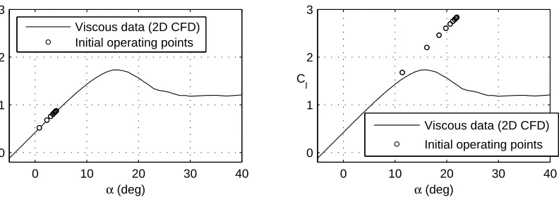
point and is denoted by (αs(j),Cls(j)). Figure 2.4 shows these initial operating

points for both a low and a high angle of attack decambering computation on a

3-D wing. In the low angle of attack case, it is seen that the starting points lie on

the input viscous data, as the solution exists in the linear aerodynamic regime. In

the high angle of attack case, the starting points lie on the potential-flowCl-αcurve

for the airfoil, which is significantly different from the viscous Cl-α curve because

of the separated boundary layer on the upper surface.

0 10 20 30 40

0 1 2 3

α (deg) C

l

Viscous data (2D CFD) Initial operating points

(a) Low angle of attack,α= 5 degrees

0 10 20 30 40

0 1 2 3

α (deg) C

l

Viscous data (2D CFD) Initial operating points

(b) High angle of attack,α= 25 degrees

Figure 2.4: Initial section operating points with δ1 = 0 degrees for low and high values

(36)

3. Calculate residual

The residual is calculated for each section. In the decambering formulation, the

residual for section j is the ∆Cl(j) between the current operating point, (αsec(j), Clsec(j)), and some unknown target point, (αt(j), Clt(j)), which lies on the viscous

input data:

F(j) = ∆Cl(j) =Clsec(j)−Clt(j) (2.6)

Unlike in a typical Newton iteration, where the residual calculation is generally via

a straightforward function evaluation, it is not clear in the current procedure how to

select the target point on the viscous curve for computing the residual. The target

point for section j will depend on the unknown decambering at other sections.

4. Modify δ1 vector

After the target points are identified for all sections and the residual vectorFis de-termined, the vector of corrections is calculated. Experience with the decambering

schemes has shown that, for a wing with N sections, rather than solve theN ×N

matrix equation (Equation 2.2) and apply the update equation (Equation 2.3) for

calculating the updates to δ1 values, it is just as effective to determine the

cor-rection vector by independent application of Equation 4.13 to the N sections. For

section j, the update toδ1 from iteration n ton+ 1 is as follows:

δ₁n+1(j) =δ₁n(j)−D ∆C n l (j)

∂Cl

∂δ1 n

(j)

(2.7)

This update approximation tends to bring down the computational cost with no

(37)

After initialization, the final three steps of the decambering procedure are repeated until

each operating point, defined to be on a strip of a lifting surface, are brought within a

specified tolerance of the input viscous Cl-α data.

Using a wing analysis method inside the solution procedure ensures that condition 1

of section 2.2 is satisfied at every iteration for the values of δ1 used in that iteration.

Once convergence is achieved, condition 2 of section 2.2 is also satisfied.

2.4 Chapter Summary

A description of the decambering concept has been provided. The method allows the

effects of flow separation to be modeled by applying a twist distribution to an airfoil or

finite wing such that the potential flow Cl matches the viscous Cl. In a two-dimensional

flow, the amount of decambering applied is straightforward to calculate. Complications

arise when applying decambering to a finite wing because of the interactions between

all sections when decambering is changed on any one section. The problem is necessarily

formulated into a Newton iteration to seek the proper amount of decambering to apply

to all sections simultaneously. The application of the Newton iteration to the problem is

non-standard due assumptions that must be made to perform the residual calculation.

(38)

Chapter 3 Comparison of Residual Calculation

Schemes

This chapter compares four residual calculation schemes as implemented in the

decam-bering approach to predict post-stall aerodynamics for finite wings. As with Chapter 2,

much of the discussion and figures in this chapter has also been adapted from Paul and

Gopalarathnam [34]. While later chapters in this document focus on implementing the

decambering calculation in an unsteady vortex lattice method, throughout the course

of this research it has been found to be enlightening to study the residual calculation

schemes using an alternate aerodynamic analysis method based on the superposition of

basic and additional aerodynamic loadings. The superposition approach is an equivalent

representation of a vortex lattice (or similar) method, and is described in Section 3.1.

Fol-lowing the brief description of the superposition approach, the four separate approaches

for the trajectory line, and the motivation behind each are presented in Section 3.2.

Af-ter the trajectory line approximations and the corresponding equations that are used for

(39)

schemes are compared against one another on the basis of computational efficiency and

rate of convergence. Two of the approaches are found to converge to nearly the same

so-lutions for the test case considered, while two are shown to be unsuitable for the problem

at hand. Due to higher computational efficiency, a particular scheme for implementation

in the vortex lattice method. The Chapter concludes by highlighting a limitation of the

decambering methodology that is independent of the residual calculation scheme utilized.

3.1 Aerodynamic Analysis Method Used to Study

the Residual Calculation Schemes

To use the decambering approach for calculating the forces and moments acting on an

aircraft, a lifting-surface aerodynamic analysis method is needed. This can be a vortex

lattice method (VLM) (as used in [26], and in subsequent chapters of this document),

Weissinger method, or similar tool. The analysis method is used to determine the

aero-dynamics for a given set of aircraft states and a given distribution ofδ1 on all the sections

of the surfaces. In the superposition approach, elementary basic and additional lift

dis-tributions are pre-computed using an analysis method and stored. For any given flight

condition, the lift distributions and aerodynamic forces and moments are computed in

the approach by linear superposition of the elementary loadings. The superposition of

basic and additional lift distributions is described in several references [36, 41, 20] and

has been used effectively for several decades in wing design [41, 42], and most recently in

flap optimization of adaptive wings [43, 44] and multiple-wing configurations [45]. The

results of [43], [44], and [45] show that the superposition approach is highly effective in

(40)

compa-rable to the original analysis method used to compute the elementary lift distributions.

A brief description of the superposition approach is provided here.

Within the assumption of linear aerodynamics (linear Cl-α variation and linear Cl

-Γ relationship), the spanwise distribution of Cl over a wing or configuration can be

expressed as a sum of two contributions: i) basic distribution, Clb(y), and ii) additional

distribution, Cla(y):

Cl(y) = Clb(y) +Cla(y) (3.1)

The basic distribution, Clb, is theCl distribution atCL= 0, and is the result of

span-wise variations in twist and flap/control deflections. Because the spanspan-wise decambering

is modeled using decambering variable δ1, it is similar to spanwise flap-angle variation,

and hence can be used to generate basic loadings.

The additional Cl distribution, Cla, is due to changes to α for the wing with zero

twist and zero decambering. The additional Cl distribution is, therefore, independent

of geometric or aerodynamic twist and it scales with wing CL. Thus, the additional Cl

distribution for CL = 1, written as Cla,1, can be precomputed for a wing and used to

compute theCla for any CL, as follows:

Cla(y) =CLCla,1(y) (3.2)

The advantage of using the superposition concept is that the net Cl distribution for

a particular wing CL can be posed in terms of the unknown decambering variables, δ1.

AssumingN sections on the wing and denoting the δ1 at sectionj byδ1,j, the expression

(41)

Cl =CLCla,1+Clb,0+Clb,1δ1,1 +Clb,2δ1,2+· · ·+Clb,Nδ1,N (3.3)

where, Clb,0 is the zero-decambering basic Cl distribution due to geometric and

aerody-namic twist resulting from spanwise changes to the wing airfoil. The increment in basic

Cl distribution due a unit δ1 for section j is denoted byClb,j.

While Equation 3.3 is expressed in terms of the wing CL, for post-stall computations

at a given wing angle of attack, αw, it is necessary to write the wingCL in terms of wing αw, as follows:

CL=a(αw−αb,0−(αb,1δ1,1+αb,2δ1,2+· · ·+αb,Nδ1,N)) (3.4)

where, a is the wing lift-curve slope (a = 1/αa,1), αb,0 is the wing angle of attack

cor-responding to the zero-decambering basic Cl distribution and αb,j is the wing angle of

attack corresponding to the increment in basic Cl distribution due a unit δ1 for section

j.

The use of the superposition approach instead of a VLM-like analysis method for the

decambering method was first proposed in [46] where additional details are available. The

approach was subsequently used for flight-dynamics simulation in [47]. More details of

the use of the superposition technique in the decambering approach and flight-dynamics

simulation are discussed in [47].

For the results presented in the Chapter, the WINGS Weissinger code was used to

compute the elementary basic and additional loadings for the superposition approach.

To illustrate the effectiveness of the superposition approach, Figure 3.1 compares the

spanwise Cl distributions for the wing-tail configuration of Figure 2.2 from the

(42)

this illustration, symmetric loadings are assumed, although the formulation is applicable

to the modeling of asymmetric loadings or asymmetric stall. Figure 3.1(a) shows the

ad-ditional loading (Cla,1) for the wing-tail configuration. Two example basic loadings due

to decambering, Clb,j, are shown, with each basic loading shown for a strip on the left

side of the aircraft added to that from its mirror-image strip on the right side to ensure

symmetry of loadings. The two basic loadings, magnified by three times for clarity, are

for strip pairs (2,19) at the wing tips and (10,11) at the wing root. Figure 3.1(b)

com-pares the total Cl distribution from superposition with direct analysis (Weissinger) for

α = 10 degrees with and without prescribed decambering. For the prescribed

decam-bering case, δ1 is set to a value of −3 degrees for the pair of strips (10,11) at the wing

root. When decambering is specified at the wing root, the loss in lift there affects the lift

distribution on the downstream tail surface. It is seen that the predicted loadings from

the superposition approach agree excellently with those from direct analysis. Of interest

as it relates to the post-stall aerodynamics is that the effect of wing decambering on the

(43)

C

la,1 distribution C

lb, δ1 = 1 degree at strips 2,19 C

lb, δ1 = 1 degree at strips 10,11 C

l

(a)

Direct analysis (no decambering) Superposition (no decambering) Direct analysis (decambering) Superposition (decambering)

C l

(b)

Figure 3.1: Comparison of spanwise Cl distributions from the superposition approach

and direct analysis (using Weissinger method) for wing-tail configuration: (a) Additional loading and two example basic loadings, with the basic loading scaled by 3 times for clarity, (b) Total loading from superposition and direct analysis for α = 10o _{with no}

decambering and with δ1 =−3o applied to wing sections 10,11 near the root.

3.2 Residual calculation schemes

This section presents the details of the four residual calculation schemes. In the discussion

for each scheme, the concept of the “trajectory line” from Section 2.2 is used to explain

how the target operating point on the viscousCl-αcurve is selected. The trajectory lines

for the four schemes are compared in Figure 3.2 for a section (section 5) of the rectangular

wing (shown in Figure 2.2) operating at α = 20 degrees with zero initial decambering.

The four trajectory lines are co-plotted from the initial operating point for this section,

(44)

0 5 10 15 20 25 30 35 40 0.4

0.6 0.8 1 1.2 1.4 1.6 1.8 2

α (deg) C

l

Starting point

Target point

Viscous data (2D CFD)

12.5 13 13.5 14 14.5 15 15.5

1.5 1.6 1.7 1.8 1.9

C l

A

B

C D

α (deg)

Figure 3.2: Comparison of the trajectory lines from the four schemes for section 5 on the wing. The initial operating point (withδ1 = 0 degrees) is for wing angle of attack of

(45)

3.2.1 Scheme A

The trajectory line used in scheme A is similar to that used in previous efforts by other

researchers [15, 18]. In this method, a vertical trajectory line is used to find the

intersec-tion with the viscous input data, as shown in Figure 3.2. The implicit assumpintersec-tion is that

the operating point for a section changes with decambering as if the section was in 2D

flow, with no induced flow due to other portions of the wing. Thus, in the calculation of

the residual, this scheme does not take into consideration any effect of the wing aspect

ratio or the spanwise location of the section on the wing. Using a wing section j for this

discussion, the decambering variableδ1(j) is updated from iterationn ton+ 1 as follows:

δ₁n+1(j) = δn₁(j)−DCl n

sec(j)−Cl n t(j) a0

(3.5)

As discussed later in Section 3.3.2, this scheme is very robust in determining a converged

solution, but requires considerable under-relaxation for convergence at some post-stall

conditions. Owing to the fact that the conditions at which under-relaxation is needed are

not known a priori, a conservative decision to use under-relaxation at all conditions is

taken, whether the conditions correspond to pre-stall or post-stall angle of attack. The

large number of iterations results in increased computational time for convergence.

3.2.2 Scheme B

Scheme B uses a sloped trajectory line following the approach presented in [26] in which

a VLM was used as the aerodynamic analysis method. This scheme was subsequently

used in [46] in which the superposition approach was used in lieu of a full aerodynamic

analysis method with the aim of decreasing computational time. The use of the

(46)

slope in this scheme are invariant with angle of attack and decambering. They need to

be calculated only once for a given geometry and discretization. To determine the slope

of this trajectory line, a small perturbation is made to the decambering of the current

section as illustrated in Figure 2.3 and the operating point for the perturbed condition is

determined by assuming that there is no change in the decambering for all the other

sec-tions of the wing. The resulting trajectory-line slope for sectionj, for which the derivation

was provided in [46], is given as:

dCl dα

traj,j

= −αb,jCla,1(j)/αa+Clb,j(j)

Clb,j(j)/a0−αb,jCla,1(j)/(αaa0)−1

(3.6)

The δ1 vector is updated from iteration n to n+ 1 as follows:

δ₁n+1(j) =δn₁(j)−D Cl n

sec−Clnt

−a0αb,jCla,1(j) +Clb,j(j)

(3.7)

Scheme B was the first scheme [26] to take three-dimensional effects into account in

computing the residuals for post-stall calculations. However, this scheme has drawbacks

of the trajectory line being sensitive to the number of sections on the wing. This scheme

also lacks robustness for certain combinations of wing aspect ratios and airfoil lift curves.

3.2.3 Scheme C

Scheme C was developed [47] with the aim of taking into consideration the effect of

decambering on all sections of the wing on the trajectory line at any given section. In

this scheme, using section j for illustration, the first iteration is made using a vertical

trajectory line (as described in scheme A) from the starting operating point with zero

decambering, (αs(j), Cls(j)). As a result of the first iteration, a new operating point is

(47)

Newton iteration step, it partially takes into consideration the changes in decambering

of all sections on the wing. The line joining (αs(j), Cls(j)) and (αp(j), Clp(j)) is the

trajectory line for section j, and is shown in Figure 3.2. The slope of the trajectory line

is determined as follows:

dCl dα

traj,j

= Clp−Cls

αp−αs

(3.8)

The update to δ1 at iteration n that will bring the operating point closer to the airfoil

Cl-α curve is as follows:

δ₁n+1(j) =δ₁n(j)−D Cl n

sec−Clnt

(Clp−Cls)/(δ1p−δ1s)

(3.9)

As discussed later in Section 3.3.2, scheme C has issues of being unable to converge

because of significantly incorrect trajectory-line slopes when some sections of the

config-uration have operating points that are converged (on the viscousCl-α curve) while other

sections are well away from convergence.

3.2.4 Scheme D

Scheme D was developed because of issues with the robustness of schemes B and C and

large computational times of scheme A. In scheme D, the trajectory lines are determined

by assuming that all sections have the same change in decambering, which is essentially

like a change in the wing angle of attack. To determine the slope of this trajectory line,

a small perturbation is made to the decambering of the current section as illustrated in

Figure 2.3 and the operating point for the perturbed condition is determined by assuming

that the same perturbation is also applied to all the other sections of the wing. The

(48)

dCl dα

traj,j

= Cla,1(j)

αa,1(j)−αa,wing

(3.10)

These trajectory lines are then used to determine the target operating points for each

section. The update to δ1 at iteration n that will bring the operating point closer to the

viscous Cl-α curve of the airfoil is as follows:

δn₁+1(j) =δ₁n(j)−D Cl n sec−Cl

n t Cla,1(j)/αa,wing

(3.11)

As discussed later in Section 3.3.2, the approximation for the trajectory-line slope

in this scheme results in a very good estimation of the target operating point on the

viscous Cl-α curve, resulting in excellent convergence even for post-stall conditions. The

estimated trajectory-line slope takes into consideration both the wing geometry (such as

aspect ratio) and the spanwise location of the section along the wing. Additionally, it does

not exhibit any undesirable sensitivity due to the discretization (number of sections). The

calculated slopes are invariant with angle of attack and decambering, because of which

they need to be determined only once, and this may be done as a pre-processing step

after which many aerodynamic inflow conditions may be evaluated. It is also shown that

no under-relaxation factor is needed for this scheme. Among the four schemes considered

in this paper, this scheme requires the minimum number of iterations for convergence at

any angle of attack. This scheme has proven to be both fast and robust.

3.3 Results and Discussion

Results are presented in this section from pre- and post-stall calculations to compare

(49)

configuration shown in Figure 2.2. The wing will be the primary focus of the study.

The tail surface has been included to illustrate convergence problems with one of the

schemes. Because the decambering approach uses airfoil lift curve as input and provides

the wing lift curve as output, validation of the approach requires the availability of

pre-and post-stall data for both airfoil pre-and wing from the same source. Owing to the dearth

of experimental data having consistent airfoil and wing lift characteristics at post-stall

conditions, a recent effort was undertaken at NC State to develop a database of results

for airfoils and wings using CFD with a Reynolds Averaged Navier Stokes (RANS) code

in time-accurate mode. For this effort, the NASA TetrUSS CFD software [48] was used

with the Spalart-Allmaras turbulence model [49], with care taken to ensure that the

grids were consistent between the simulations for the 2D (airfoils) and the 3D (wings)

geometries. More details of the approach and early results from the effort are documented

in Ref. [50]. The RANS CFD computations were performed for the wing alone (without

the tail surface) to keep computational costs low. Because of the negligible influence of

the tail on the wing aerodynamics, the comparison of wing-onlyCLresults from the four

residual-computation schemes applied to wing+tail geometries with CFD results for the

wing-alone geometries is adequate for validation of the low-order method.

The comparison of the predicted lift curves for the wing from the four schemes with

CFD results is presented in Section 3.3.1 along with results comparing the four schemes

based on the number of iterations needed for convergence. It is shown that schemes B

and C do not converge for certain situations even with under-relaxation. Section 3.3.2

next presents an explanation of the observed behavior of the four schemes by comparing

the trajectory lines and the “evolution” of the solution from the initial to the converged

solution. Section 3.3.3 then compares the effects of initial value of the decambering on

(50)

0 5 10 15 20 25 30 35 40 0.2

0.4 0.6 0.8 1 1.2 1.4 1.6 1.8

α (deg)

C_l, C_L Scheme Bfails for

α > 16 deg

Scheme C fails for

α > 19 deg

Scheme A uses damping

for α = 24, 25 deg 2D CFD

3D CFD Scheme A Scheme B Scheme C Scheme D

Figure 3.3: Wing-only CL-α curves from schemes A–D compared with 2D and 3D CFD results.

robust, but also the most computationally efficient. Section 3.3.4 compares the spanwise

distributions of lift coefficient from scheme D with those from CFD for several angles

of attack, highlighting interesting features of the solution. Finally, section 3.3.5 presents

the effect of sweep angle on the stall characteristics to illustrate the limitations of the

current decambering approach.

3.3.1 Comparison of residual calculation schemes

The results from CFD were computed at a Reynolds number of 3.0 million for the NACA

4415 airfoil and the aspect ratio 12 constant-chord wing. Figure 3.3 shows the wing-only

CL vs.α curves for the wing-tail configuration computed using each residual calculation

scheme. For these decambering calculations, the 2D lift curves from CFD were used as

Low-Order Post-Stall Aerodynamics Modeling for use in Flight Simulation and Stability Analysis.

ABSTRACT

DEDICATION

BIOGRAPHY

ACKNOWLEDGEMENTS

TABLE OF CONTENTS

LIST OF TABLES

LIST OF FIGURES

LIST OF SYMBOLS, ABBREV., NOMENCLATURE

Chapter 1

Introduction

1.1

Literature Review

1.1.1

Post-Stall Corrections in Potential Flow Aerodynamics

Analysis Methods

1.1.2

Aerodynamics in the Loop

1.1.3

Stability Analysis

1.2

Layout of the Document

Chapter 2

The Decambering Post-Stall

Aerodynamic Model

2.1

Decambering Applied to a 2D Flow

2.2

Decambering in a 3D Flow

2.3

Solution Procedure for Applying Decambering

to a 3D Wing

2.3.1

The General Form of a Newton Iteration

2.3.2

Applying the General Form of a Newton Iteration to

Post-Stall Wing Aerodynamics

2.4

Chapter Summary

Chapter 3

Comparison of Residual Calculation

Schemes

3.1

Aerodynamic Analysis Method Used to Study

the Residual Calculation Schemes

3.2

Residual calculation schemes

3.2.1

Scheme A

3.2.2

Scheme B

3.2.3

Scheme C

3.2.4

Scheme D

3.3

Results and Discussion

3.3.1

Comparison of residual calculation schemes