INVESTIGATION
Combining Markers into Haplotypes Can Improve
Population Structure Inference
Lucie M. Gattepaille* and Mattias Jakobsson*,†,1
*Department of Evolutionary Biology, Evolutionary Biology Centre, and†Science for Life Laboratory, Uppsala University, SE-752 36, Uppsala, Sweden
ABSTRACTHigh-throughput genotyping and sequencing technologies can generate dense sets of genetic markers for large numbers of individuals. For most species, these data will contain many markers in linkage disequilibrium (LD). To utilize such data for population structure inference, we investigate the use of haplotypes constructed by combining the alleles at single-nucleotide polymorphisms (SNPs). We introduce a statistic derived from information theory, thegain of informativeness for assignment(GIA), which quantifies the additional information for assigning individuals to populations using haplotype data compared to using individual loci separately. Using a two-loci–two-allele model, we demonstrate that combining markers in linkage equilibrium into haplotypes always leads to non-positive GIA, suggesting that combining the two markers is not advantageous for ancestry inference. However, for loci in LD, GIA is often positive, suggesting that assignment can be improved by combining markers into haplotypes. Using GIA as a criterion for combining markers into haplotypes, we demonstrate for simulated data a significant improvement of assigning individuals to candidate populations. For the many cases that we investigate, incorrect assignment was reduced between 26% and 97% using haplotype data. For empirical data from French and German individuals, the incorrectly assigned individuals can, for example, be decreased by 73% using haplotypes. Our results can be useful for challenging population structure and assignment problems, in particular for studies where large-scale population–genomic data are available.
S
TRUCTURE of populations and assigning individuals to populations have attracted considerable attention in population genetics, conservation biology, and ecology (Pritchard et al.2000; Beaumont 2004; Manelet al.2005; Platt et al. 2010). Since the introduction of Wright’s FST (Wright 1921, 1943), numerous studies of population struc-ture have been conducted for a multitude of species, using a variety of genetic or phenotypic markers. The recent de-velopment of high-throughput genotyping and sequencing technologies has resulted in a substantial increase in studies of population structure that are based on a large number of markers (e.g., Jakobssonet al.2008; Plattet al.2010; Von-holdt et al. 2010). At the same time, powerful clustering methods have been developed to infer population structure on the basis of multiloci genetic data (e.g., Pritchardet al.2000; Dawson and Belkhir 2001; Corander et al. 2003;
François et al. 2006; Huelsenbeck and Andolfatto 2007; Alexander et al.2009).
For most species, individuals rarely reproduce at random and this can create genetically differentiated subgroups within a population or species. Geographic barriers such as mountains, rivers, and oceans can furthermore hinder random mating, thereby causing populations to be struc-tured (Haleet al.2001; Rosenberget al.2005). In humans, cultural differences, such as language or religious beliefs, may play an additional role in shaping structure among individuals (Cavalli-Sforza and Feldman 2003; Beharet al.
2010; Bryc et al. 2010). Large efforts have been made to characterize population structure, both at the global level (e.g., Rosenberget al.2002; Jakobssonet al.2008; Liet al.
2008) and at smaller scales (e.g., Rosenberg et al. 2006; Wang et al. 2007; Friedlaender et al. 2008; Novembre
et al. 2008; Segurelet al.2008; Reichet al. 2009; Tishkoff
et al.2009). Although population structure can give impor-tant information on the demographic history of a species and may lead to better understanding of evolutionary pro-cesses, population structure may also complicate certain investigations. For example, cryptic population structure Copyright © 2012 by the Genetics Society of America
doi: 10.1534/genetics.111.131136
Manuscript received May 26, 2011; accepted for publication August 11, 2011
1Corresponding author: Department of Evolutionary Biology, Uppsala University,
can lead to false positives in association studies (Marchini
et al.2004). Another problem may arise in forensics: if a sus-pect originates from a population that is genetically differ-entiated from the reference population, the difference in allele frequencies may lead to incorrect conclusions about matching DNA evidence to a suspect (Balding and Nichols 1994; Weir 1996; Aitken and Taroni 2004).
Assignment methods, in contrast to clustering methods, use prior knowledge about candidate groups in addition to genetic data to assign individuals of unknown origin to groups (Paetkauet al.1995; Manelet al.2005). These meth-ods have been extensively used for conservation manage-ment (see, e.g., Wasser et al. 2004; Gaskin et al. 2009) and parentage analysis (see,e.g., Nielsenet al.2001). Meth-ods that focus on finding potential hybrids of particular types (e.g.,first-generation offspring and backcrosses) have also been developed (Anderson and Thompson 2002) and used for identifying hybrids between closely related species (Adams et al.2007).
High-throughput sequencing and genotyping methods have generated dense sets of single-nucleotide polymor-phisms (SNPs) for large samples of individuals for several organisms. Linkage disequilibrium (LD) is strong for many SNPs in these dense sets (for most species), and these SNPs are therefore not independent markers. To overcome the problem of LD, some studies prune the set of SNPs before inferring population structure (e.g., Novembre et al.2008; Bryc et al. 2010) and some studies analyze subsets of markers and combine the results for different subsets (Jakobsson et al. 2008). These approaches of overcoming the problem caused by closely linked markers do not take full advantage of all the information provided by the large number of SNPs. Instead, it may be possible to combine SNPs into haplotypes, which may integrate extra informa-tion about ancestry, potentially from recombinainforma-tion events that should in principle harbor information about ancestry similar to mutation events. A previous study utilized haplo-types for revealing population structure, which point at somewhat different inference of population structure for SNPs and haplotypes (Jakobsson et al. 2008). Using simu-lations, Morin et al.(2009) demonstrated greater power of population structure inference using haplotypes in many, but not all, cases. However, it is unclear whether, and under which conditions, haplotypes can be more powerful than single SNPs for inferring population structure or assigning individuals to populations.
In this article, wefirst investigate whether haplotype data can increase the statistical power of assigning individuals to populations compared to SNP data. Second, using a newly developed statistic, the gain of informativeness for assign-ment (GIA), we characterize under which circumstances it may be advantageous to use haplotypes compared to using SNPs for ancestry inference. Third, we demonstrate by sim-ulations and by using empirical SNP data from Europeans that assignment of individuals significantly improves through combining SNPs into haplotypes guided by GIA.
Theory
We define a“haplotype locus”as the combination of more than one SNP locus. The SNP loci in a haplotype locus are not required to be consecutive along the chromosome. We define a “haplotype allele” as a particular combination of alleles at the SNP loci constituting the haplotype locus. For instance, for a haplotype locus formed by x SNPs, 2x distinct alleles can exist, but the number of observed haplo-type alleles is typically much smaller than 2xifxis reason-ably large. In addition, the number of distinct haplotype alleles is upwardly bounded by the sample size.
To develop a statistic that quantifies under which circum-stances it is advantageous for ancestry inference to combine markers into haplotype loci, we start by considering a model of two multiallelic loci denoted locus Aand locus B. The combination of the two loci into a haplotype locus is denoted locusH, and the possible haplotype alleles are the combinations of alleles from locusAand locusB(see Figure 1 for notation). Note that this model can be generalized to handle any number of markers by recursively merging two loci into one multiallelic haplotype locus. LociAandBmay be in LD, which can, for example, be quantified with theD
statistic (Lewontin and Kojima 1960). We consider K ran-domly mating populations and we assume that the allele frequencies at each locus in each population are known.
Rosenberget al. (2003) derived a criterion on the basis of information theory to evaluate the efficiency of a marker for assigning individuals to one ofKpopulations. This criterion, the
informativeness for assignment(IA), can be computed for bi- or multiallelic loci, such as SNPs, microsatellites, or haplotype loci,
IA¼X
N
j¼1 0
@2pjlogpjþ
XK
i¼1 pðjiÞ
Klogp ðiÞ j
1
A ; (1)
where N is the number of alleles for the locus, K is the number of populations, pðjiÞ is the frequency of allele j in populationi, andpjis the average frequency of allelejacross populations,
pj¼X K
i¼1 pðjiÞ
K:
Using the IA statistic, we define the GIA as
GIA¼IAðHÞ2½IAðAÞ þIAðBÞ; (2)
where IA(H) is the informativeness for assignment of the hap-lotype locus and IA(A) and IA(B) are the informativeness of locusAand locusB, respectively. Since IA is nonnegative and bounded upward by logK, GIA is restricted to [22 logK, logK]. By comparing the information content about ancestry of the haplotype to the sum of the information content of each marker, GIA is specifically designed to answer the question of whether two markers can improve the power of assigning individuals to candidate populations by combining the markers into a haplotype locus. As can been seen from Equations 1 and 2, to compute GIA, we need to know the allele frequencies of the two loci and the allele frequencies of the haplotype locus. When addressing assignment problems, phased data from candidate populations can typically be used to estimate the SNP and haplotype allele frequencies, followed by the use of GIA to determine which loci to combine to haplotype loci for optimal power. Guided by this information, individuals of unknown origin could then be assigned to candidate popula-tions on the basis of haplotype data (see the results section for explicit examples of this procedure).
GIA is not a simple function of the allele frequencies and the haplotype allele frequencies. For example, the sign of GIA cannot be determined by a simple rule of thumb based on allele frequencies. However, for the special case of biallelic markers, we can show that when two loci are in linkage equilibrium, GIA # 0. To arrive at that result, we note that because the loci are biallelic, only the frequencies of one allele for each locus are needed to characterize GIA. Recall also thatDcan be defined as the difference between the frequency of a haplotype allele and the product of the frequencies of its constitutive alleles so that haplotype allele frequencies in Equation 2 can be replaced byDand allele fre-quencies (e.g.,x11=a1b1+D).
Theorem. Let A and B be two biallelic loci and H be their associated haplotype locus. Consider K randomly mating pop-ulations. For population i,let að1iÞand bð1iÞbe the allele frequen-cies at locus A and locus B, respectively. Then, for all the frequency distributions of the alleles,
"i21 . . . K; Di¼0⇒GIA¼IAðHÞ2IAðAÞ2IAðBÞ#0
with equality if and only if PKi¼1 Pi
k¼1ðað iÞ 1 2að
kÞ 1 Þ ðbð1iÞ2bð
kÞ 1 Þ ¼0.
A proof of the Theorem is given in the Appendix. This Theorem demonstrates that when locus Aand locus B are in linkage equilibrium within all populations, the haplotype locusHprovides less information (or the same amount) for
assigning individuals to populations than locusAand locusB
provide when used separately. Intuitively, since there is no cor-relation between the allele frequencies at locusAand the allele frequencies at locusB, we expect the combination of alleles into haplotype alleles to arise randomly within each population.
GIA for two populations
We study Equation 2 for the two-population case (K= 2) and for two biallelic markers. To reduce the complexity of the problem, we assume that the level of LD is dominated by linkage of the two markers and that the two populations have similar demographic histories, so that D1 =D2= D. Five parameters characterize our problem:D,að11Þ,a1ð2Þ,bð11Þ, and bð12Þ. The haplotype allele frequencies must be greater than or equal to zero in both populations, which limits the range ofDand the range of the allele frequencies at locusA
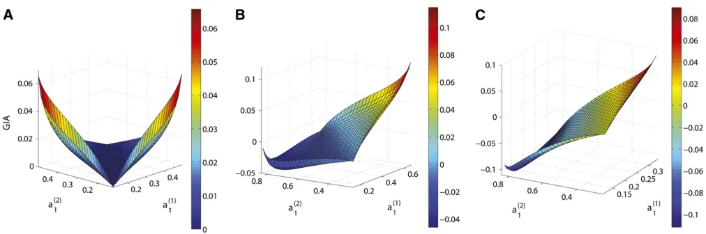
and locusB; constraints are summarized in Table 1. As an example, we study the behavior of GIA as a function ofað11Þ and að12Þ forD = 0.1 and different fixed values of bð
1Þ 1 and
bð12Þ. Figure 2 shows that GIA is positive for some parts of the parameter space, but it can also be negative, depending on the valuesað11Þ,a
ð2Þ 1 ,b
ð1Þ 1 , andb
ð2Þ
1 . Figure 2A shows the val-ues of GIA whenbð11Þ¼b
ð2Þ
1 ¼0:2 andD= 0.1 for the entire range of possible values of að11Þ and a
ð2Þ
1 , a case in which locus B is uninformative on its own [IA(B) = 0] since it has identical allele frequencies in both populations. GIA is nonnegative for all possible values of að11Þ and að12Þ, which means that the haplotype locus contains more information for assigning individuals to populations than the two loci used separately. The intuition behind this result is that locus
Ahas only two alleles, whereas the haplotype locus can have up to four different alleles, increasing the possibility for the haplotype alleles to uniquely characterize populations, which makes the assignment of individuals easier.
Figure 2, B and C, shows that the sign and magnitude of GIA varies depending on the values of the allele frequencies at locus A. The borders of the surfaces are defined by the constraints on að11Þ and a
ð2Þ
1 given in Table 1 and at each border of the surfaces, at least one haplotype allele fre-quency equals zero in one of the two populations,i.e., pri-vate for one population. There are two interesting points on the surfaces, the leftmost tip and the rightmost tip. Although they share the same property of being the only cases where two haplotype alleles are private, the rightmost tip yields the
Table 1 Constraints on Dand allele frequencies for locusAand locusBto ensure admissibility of haplotype allele frequencies in populationi
Constraints
Sign ofD OnD Onb1D Ona1jD,b1
Positive D
#1
4 b121
2
#pffiffiffiffiffiffiffiffiffiffiffiffiffi124D D
12b1
#a1#12
D b1
Negative D$21
4 b121
2
#pffiffiffiffiffiffiffiffiffiffiffiffiffiffiffi1þ4D 2bD 1
#a1$1þ D
12b1
maximum GIA whereas the leftmost tip yields a negative GIA. The absolute differencejað11Þ2a
ð2Þ
1 jdistinguishes the two points, which is greater for the leftmost tip, resulting in a greater IA(A) and therefore a smaller GIA than for the rightmost tip. Never-theless, they are both local maxima, which is caused by the often substantial informativeness of private alleles.
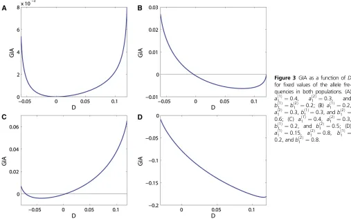
We also investigate the behavior of GIA as a function ofD
when all the allele frequencies arefixed and GIA is therefore completely determined by IA(H). Figure 3 shows four exam-ples of GIA as functions of D, across the range of possible values ofD, for different values ofað11Þ,að
2Þ 1 ,bð
1Þ 1 , andbð
2Þ 1 . We first observe that if D = 0, GIA # 0 (consistent with the Theorem). For að11Þ¼0:4, að
2Þ
1 ¼0:3, and bð 1Þ 1 ¼bð
2Þ 1 ¼0:2 (Figure 3A), GIA is nonnegative for the whole range of D. This example is similar to the example in Figure 2A, for which locus B was also uninformative.
The sign and the magnitude of GIA varies as a function of
Dforfixed allele frequencies of locusAand locusB. GIA can be positive for the entire range ofD(Figure 3A), negative for the entire range (Figure 3D), or change sign depending onD
(Figure 3, B and C). The range of Dis defined by the con-straints that all haplotype allele frequencies have to be non-negative. The two extreme values for each case in Figure 3 correspond to one of the eight haplotype allele frequencies (four haplotype allele frequencies in each population) being equal to zero in one population, which means being a private allele for the other population.
In summary, although there are a number of predictable behaviors of GIA—such as that GIA#0 when markers are in linkage equilibrium and that GIA is often large for cases where private alleles exist—GIA is not a trivial function of LD or allele frequencies.
Results
Comparing GIA and performance of assignment
To assess how haplotype loci that are constructed on the basis of GIA perform for assigning individuals to populations,
we evaluate assignment in a two-population case for a wide range of allele frequencies and levels of linkage disequi-librium. We investigate a case of 200 haploid individuals, 100 individuals from each population, where each individual is assumed to be typed for 40 pairs of SNPs. We generate a discrete set of haploid gene copies (for a pair of SNPs) for each population that satisfies a particular choice of allele frequencies and levels of LD (see Table 2). This set of gene copies is randomly permuted to generate a set of 40 pairs of SNPs, which ensures that the pairs of SNPs are independent of each other (conditional on the allele frequencies). This procedure guarantees that all the SNP pairs have the same allele frequencies for SNPA, SNPB, and theA–B haplotype locus and consequently the same level of LD between the two SNPs. Note that within a population, most of the LD in the sample is a result of the linkage between the two SNPs in each pair.
For these population-genetic data, we use the software STRUCTURE (Pritchardet al.2000; Falushet al.2003), to assign the 200 haploid individuals to two clusters (no-admixture model, burn-in period of 20,000 iterations followed by 5,000 iterations from which estimates were obtained), using either the 80 SNPs or the 40 haplotype loci obtained by combining each pair of SNPs into one haplotype locus. From the STRUCTURE result, the mean incorrect assign-ment proportion (MIAP) is computed, which is the average proportion of individuals that are assigned to the incorrect population. For a given set of allele frequencies, we generate 100 different replicate samples using the data-randomization procedure described above, assign individuals to populations, and compute the average (across replicates) of MIAP. For comparison,FSTvalues for the SNP pairs, as well asFSTvalues for the haplotype loci, are computed. Similarly to IA,FSTalso relies on information about allele frequencies.
Table 2 shows the performance of the assignment based on the 80 SNPs and based on the 40 haplotype loci for various choices of allele frequencies and levels of LD. In most cases when GIA is positive, the MIAP values are lower
Figure 2 GIA as a function ofað1Þ
1 , a
ð2Þ
1 , whenD ¼0.1, for differentfixed values ofb ð1Þ
1 andb
ð2Þ 1 . (A)b
ð1Þ
1 ¼0:2 andb ð2Þ
1 ¼0:2; (B)b ð1Þ
1 ¼0:3
andbð2Þ
1 ¼0:6; (C)b ð1Þ
1 ¼0:15 andb ð2Þ
for the haplotype loci than for the SNPs. Similarly, when GIA is negative, the MIAP values are in most cases lower for the SNPs than for the haplotype loci. For the choices of allele frequencies and levels of LD in Table 2, Figure 4 shows the difference between the MIAP based on SNPs and the MIAP based on haplotype loci (i.e., improved assignment due to haplotype loci) as a function of GIA (Figure 4A), the mean (across populations) ofjDj(jDj, Figure 4B), the mean (across populations) ofr2(r2, Figure 4C), and the difference inF
ST between the 40 haplotype loci and the 80 SNPs (Figure 4D). The improved assignment due to using haplotype loci is pos-itively correlated with GIA (Pearson’sr = 0.748, P = 4· 1025), and the correlation is nonsignificant withjDjandr2 (r=20.289,P= 0.16 andr=20.302,P= 0.18, respec-tively). The improved assignment is neither correlated with
FSTfor haplotype loci nor correlated withFSTfor SNPs (r= 20.037,P= 087 andr= 0.401,P= 0.06, respectively), but it is positively correlated with the difference betweenFSTfor haplotype loci and FSTfor SNPs (r = 0.790,P= 7·1026). GIA and the difference inFSTvalues appear to be good indi-cators of how assignment can be improved by combining SNPs into a haplotype loci. The outlier observed far from the regression line in Figure 4A corresponds to the 10th entry in Table 2. For this set of allele frequencies, 40 pairs of SNPs are enough to obtain a very accurate assignment (MIAP close to 0) and there is not much room for improvement when combining the SNPs into haplotype loci. GIA and the differ-ence inFSTvalues are correlated (r= 0.792), suggesting that
the two statistics contain similar information despite the fact that GIA is based on a measure of information whereas FST measures differentiation, but there are similarities of the two statistics as well. Indeed, if the differentiation between the two populations is easier to capture when considering haplo-type loci compared to considering SNPs separately, we would expect that assignment also improves for haplotype data com-pared to SNP data.
Improving assignment using GIA—a simulation study
For empirical population genetic data, allele frequencies and levels of LD vary extensively among loci. GIA is defined for multiallelic markers and can be used for assessing the usefulness of combining not only pairs of SNPs, but also haplotype loci themselves. Thus, GIA can be used for large numbers of SNPs. To demonstrate the utility of GIA, we compare the results of the assignment of 200 haploid individuals originating from two populations and based on 1000 SNPs using different strategies of dealing with the SNPs, e.g., by pruning the SNPs or combining them into haplotype loci. We simulate the 200 haploid individuals with the software ms (Hudson 2002) from a two-island model with migration rate m (migrants per generation) and an effective population size of 1000. Each haploid in-dividual represents a DNA fragment of 4.2 Mb with a total scaled recombination rate ofr= 4Nr= 150 orr= 4Nr= 1500 (where Nis the population size andris the recombi-nation rate per generation for the entire fragment). We
Figure 3 GIA as a function ofD for fixed values of the allele fre-quencies in both populations. (A)
að1Þ
1 ¼0:4, a
ð2Þ
1 ¼0:3, and
bð1Þ
1 ¼b
ð2Þ
1 ¼0:2; (B) a ð1Þ
1 ¼0:2,
að2Þ
1 ¼0:3,b
ð1Þ
1 ¼0:3, andb ð2Þ
1 ¼
0:6; (C) að1Þ
1 ¼0:4, a
ð2Þ
1 ¼0:3,
bð1Þ
1 ¼0:2, and b ð2Þ
1 ¼0:5; (D)
að1Þ
1 ¼0:15, a
ð2Þ
1 ¼0:8, b
ð1Þ
1 ¼
0:2, andbð2Þ
repeat the simulation 100 times for a given migration rate and a given recombination rate. For each sample, we assign the 200 individuals using STRUCTURE on the basis of seven different treatments of the SNPs:
1. Using all 1000 SNPs.
2. Using a subset of the SNPs obtained by pruning. We prune the set of SNPs with the program PLINK (Purcell
et al.2007), to remove SNPs that are in high LD (rejec-tion threshold of r2 = 0.1, windows of 20 SNPs, and shifts of 5 SNPs).
3. Combining the SNPs into haplotype loci with a greedy algorithm that recursively combines the pair of loci that has the greatest GIA among all the pairwise comparisons of loci until no remaining pair of loci has a positive GIA. We refer to this strategy as MaxGIA.
4. Using a set of randomly formed haplotype loci with a haplotype length distribution matching the haplotype length distribution of the set in c. We call this strategy RandomHaplotypes.
5. Using the set of SNPs and haplotype loci obtained with the following algorithm: starting at thefirst SNP, if GIA is positive between SNP 1 and SNP 2, combine them into a haplotype. Compute GIA for the SNP 1–SNP 2 haplo-type and SNP 3, and combine them into a haplohaplo-type if GIA is positive. Repeat this process until a SNPsis found for which the haplotype locus and SNPshave a nonpos-itive GIA. Repeat the process starting from SNP s. We refer to this strategy as NeighborGIA.
6. Using a set of haplotype loci formed by neighboring SNPs obtained by randomly permuting the breakpoints of the haplotype loci set in e, so that the haplotype length dis-tribution is the same as in e. We call this strategy RandomNeighbor.
7. Combining the SNPs into haplotype loci with a greedy algorithm that recursively combines the pair of loci that has the greatestd=FST(H)2FST(M1, M2) among all the pairwise comparisons of loci until no remaining pair of loci has a positived.FST(H) denotesFSTfor a haplotype locus, and FST(M1, M2) denotes FST computed for the two markers constituting the haplotype loci. We refer to this strategy as MaxFST.
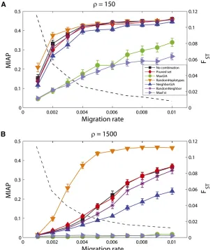
For each sample, migration rate, and strategy, we record the performance of assigning individuals to populations that is obtained from STRUCTURE (with the same settings as above). Figure 5 shows MIAP for the different strategies (no combination, pruning, MaxGIA, RandomHaplotypes, NeighborGIA, RandomNeighbor, and MaxFST) for a range of migration rates m and scaled recombination rates of r= 150 andr= 1500. The GIA- and the FST-based strate-gies require some knowledge about allele frequencies for the considered markers, including the haplotype loci formed in the iterative processes. In the context of an assignment problem, this information can be obtained from phased data for candidate populations. In this simulation study, we estimate the allele frequencies directly from the sample and use our knowledge of the individuals’ true ancestry. Thus,
Table 2 The mean incorrect assignment proportion (MIAP) obtained by assigning 200 haploid individuals to either of two populations using STRUCTURE based on 80 SNPs, or based on 40 haplotype loci, and for various allele frequencies and levels of LD
að1Þ
1 a
ð2Þ
1 b
ð1Þ
1 b
ð2Þ
1 jDj r2 GIA MIAP SNPs MIAP hapl. FST(SNPs) FST(hapl.)
0.41 0.60 0.17 0.05 1.5·1024 1.3·1026 26.29·1024 0.0976 0.1209 0.0606 0.0498
0.62 0.81 0.38 0.25 0.0384 0.0500 1.59·1022 0.1212 0.0719 0.0517 0.0844
0.38 0.17 0.11 0.15 0.0413 0.0998 1.03·1022 0.1642 0.1140 0.0612 0.0689
0.47 0.32 0.21 0.12 0.0685 0.1500 1.07·1022 0.4286 0.1519 0.0301 0.0589
0.11 0.23 0.26 0.18 0.0514 0.1846 7.55·1022 0.4186 0.0015 0.0229 0.0568
0.05 0.01 0.13 0.05 0.0215 0.2004 23.23·1023 0.2422 0.2625 0.0257 0.0226
0.61 0.88 0.15 0.03 0.0589 0.2514 22.19·1022 0.0372 0.0460 0.1400 0.1168
0.31 0.35 0.23 0.30 0.1018 0.2981 3.01·1022 0.4736 0.1376 20.0022 0.0260
0.08 0.21 0.03 0.11 0.0522 0.3599 28.53·1023 0.1740 0.1988 0.0503 0.0419
0.38 0.17 0.11 0.23 0.0895 0.3659 5.78·1022 0.0444 0.0047 0.0731 0.0901
0.04 0.08 0.05 0.08 0.0222 0.3996 5.33·1022 0.3738 0.0353 6.17·1024 0.0527
0.71 0.61 0.60 0.49 0.1575 0.4560 23.96·1023 0.4205 0.4962 0.0133 0.0081
0.28 0.14 0.25 0.22 0.1196 0.4974 8.11·1023 0.3747 0.2859 0.0194 0.0133
0.05 0.01 0.11 0.01 0.0172 0.5645 6.02·1023 0.1701 0.0768 0.0562 0.0687
0.18 0.36 0.28 0.37 0.1582 0.6043 2.12·1022 0.2387 0.0851 0.0378 0.0460
0.17 0.37 0.13 0.25 0.1327 0.6486 21.07·1022 0.1516 0.1618 0.0653 0.0597
0.14 0.34 0.19 0.38 0.1521 0.6913 21.75·1022 0.1042 0.1251 0.0848 0.0733
0.01 0.06 0.99 0.89 0.0316 0.7582 27.37·1023 0.1759 0.1227 0.0576 0.0539
0.33 0.26 0.33 0.24 0.1843 0.8138 22.45·1023 0.4545 0.4920 0.0057 0.0044
0.08 0.10 0.08 0.14 0.0798 0.8413 9.66·1023 0.4378 0.2871 0.0011 0.0040
0.06 0.08 0.06 0.10 0.0642 0.8913 4.35·1023 0.4408 0.3645 20.0028 20.0020
0.28 0.07 0.28 0.07 0.1283 0.9516 23.5·1022 0.0483 0.0474 0.1332 0.1294
0.81 0.69 0.81 0.69 0.1839 1 29.67·1023 0.3272 0.4344 0.0280 0.0280
Values ofjDjandr2are means across populations. The values presented are averages across 100 replicate cases. GIA,F
STbased on the 80 SNPs, andFSTbased on the 40
haplotype loci are given for comparison.FSTvalues are computed using equation 5.3 in Weir (1996). For MIAP, the smallest values between SNPs and haplotypes of incorrect
improvement based on the GIA or theFSTstrategy is to some degree magnified by the fact that we are using information about the individuals’ true ancestry to compute the allele frequencies. However, the NeighborGIA strategy uses the same information as the MaxGIA and MaxFST strategies, and the improvement obtained for the MaxGIA and MaxFST
strategies cannot be explained solely by using information about the individuals’ancestry.
For both recombination rates, the MaxGIA and MaxFST strategies for combining SNPs show the fewest incorrect assignments, but recombination rate has a strong impact on the accuracy of the assignment. For the high-recombination
Figure 4 The difference in assignment accuracy (MIAP) based on SNPs and haplotypes as a function of GIA, LD (jDjandr2), and the difference between
FSTfor haplotype loci andFSTfor SNPs (values are given in Table 2). A linear regression line is included for each comparison. (A) GIA,r¼0.748,y¼4.1x+
0.046 (P¼4·1025); (B)jDj,r¼20.302,y¼20.75x+ 0.14 (P¼0.16); (C)r2,r¼20.289,y¼20.13x+ 0.14 (P¼0.18); (D)F
ST(Haplotypes)2FST(SNPs), r¼0.790,y¼6.1x+ 0.040 (P¼7·1026).
Figure 5 Mean incorrect assignment proportion (MIAP) computed on the basis of assignment of 200 individuals using STRUCTURE for different strategies of combining SNPs and for different migration rates. A total of 1000 SNPs for a fragment of DNA are simulated for 200 haploid individuals, 100 from each of two populations, and with a scaled recombination rate (r) of 150 (A) or 1500 (B) for the entire DNA fragment. MIAP values are averages across 100 replicate simulations and error bars give the interval
61.96 times the standard error of the mean. MeanFST
case (r= 1500), the markers are less correlated and the set of markers carries more information about ancestry than the markers in the low-recombination case. Furthermore, as expected, when the migration rate increases (and FST decreases), MIAP also increases for all seven strategies. However, for the high-recombination case and a migration rate of 0.01, the MaxGIA and MaxFSTstrategies can uncover the structure with (on average),2% incorrect assignment compared to 37% using the full set or the pruned set of SNPs (Figure 5B). Combining neighboring SNPs that have positive GIA also improves the assignment, but to a lesser extent than the MaxGIA strategy. For both choices of recombination rates, the strategies that combine SNPs into haplotypes in a random manner (RandomHaplotypes and RandomNeighbor) result in poor assignment. Thus, the improved assignment for MaxGIA, and to some degree NeighborGIA, compared to the pruning or no combination strategies is likely to be the result of using GIA as a criterion for combining SNPs into haplotypes and not just a result of randomly combining SNPs into haplotypes. However, for r= 1500, the strategy RandomNeighbor, which consists of randomly combining neighboring SNPs, increases the accuracy of the assignment compared to the pruning or no combination strategies. Fi-nally, we note that the accuracy of the assignment for the pruned set of SNPs is similar to that of the assignment based on the full set of SNPs, suggesting that the removed SNPs contained redundant information about ancestry.
In the case of 1% migrants per generation (m= 0.01, the greatest migration rate that we investigate), the distribution of MIAP for the 100 replicates varies depending on the
strat-egy for treating the SNP data. Six distributions of MIAP (based on different treatments of the SNPs) for the low-recombination case (r= 150) are shown in Figure 6 and the corresponding distributions of MIAP for the high-recombination case (r = 1500) are shown in Figure 7. Forr= 150, the distribution of MIAP based on the MaxGIA strategy is spread over a range of values compared to the results of the other strategies, which are skewed toward 0.5, the expected value of MIAP for random assignment of individuals to populations (but note that this expected value may be slightly smaller for finite population sizes and un-labeled populations). So, as also shown by the mean MIAP in Figure 5A, MaxGIA is the most accurate strategy, but there are also cases of poor assignment using this strategy. If we increase the recombination rate, all six distributions of MIAP move away from 0.5, except for RandomHaplotypes. The distributions of MIAP for RandomNeighbor, pruning, or no combination strategies are similar and have large variances. The distribution of MIAP for the MaxGIA strategy is skewed toward 0, demonstrating superior assignment accuracy com-pared to the other strategies.
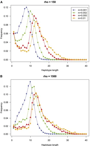
To get an idea of how many SNPs make up the haplotype loci that are constructed using the MaxGIA strategy, we compute the distribution of the number of SNPs in haplo-type loci for four different migration rates and for two different recombination rates (Figure 8). All the length dis-tributions show a clear mode, and the value of the mode appears to increase with increasing migration rate. This observation suggests that when it becomes more difficult to assign individuals to populations because of higher
Figure 6 Histograms of the mean incorrect assignment prob-abilities (MIAP) for 100 replicates of simulated data from a two-island-model with migration rate
migration rate, longer haplotype loci may increase the accu-racy of the assignment. For the low-recombination case (r= 150), there is also a second mode at one single SNP (for all but the lowest migration rate), showing that many SNPs are not combined with other SNPs for these cases. In general, however, the recombination rate appears to have little impact on the length distribution of the majority of haplotype loci.
Improving assignment using GIA—POPRES data
To investigate whether haplotype loci can improve ancestry inference for empirical population genetic data, we use SNP-chip data from the POPRES panel that contain some 1385 individuals from Europe (Nelson et al. 2008), which have been genotyped for some 500,000 SNPs. We phased all indi-viduals using fastPHASE (Scheet and Stephens 2006), ver-sion 1.4 (“haplotype clusters”set to 20 and 20 runs of the EM algorithm), which generated “best guess”estimates of the phase of each of the two haploid copies for each individual.
We conduct a cross-validation study for the 89 French and 70 German individuals (one German outlier individual was removed) in the POPRES collection (Nelsonet al.2008) and focus on the phased data of 105,341 SNPs on chromosomes 1, 2 and 3 (FST= 0.00068). To construct a training set, 45 French individuals and 35 German individuals were ran-domly sampled, and the remaining 44 French and 35 German individuals make up the validation set. Each chromosome is divided into windows of 10 SNPs and using the MaxGIA strategy, we build a set of haplotype loci using estimated allele frequencies from the training set of individuals for each
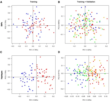
10 SNP-window. This set contains 54,762 haplotype loci and the configuration of SNPs is known so that we can combine the SNPs in the validation set to make up the same haplotype loci. We perform the assignment of the individuals in the validation set using STRUCTURE and using principal compo-nent analysis (PCA), for either the entire set of SNPs or the set of haplotype loci. For STRUCTURE, we compute the frac-tion of the validafrac-tion individuals that are misclassified using the training individuals as known populations (supervised clustering), as well as the fraction of misclassified individuals in the training set alone (based on unsupervised clustering). There was no obvious clustering of individuals in the training set using either SNPs or haplotype loci (50% correctly classified individuals for both types of data). Assigning individuals in the validation sets also performs poorly for both haplotype loci (51% correctly classified individuals) and SNPs (61% correctly classified individuals). However, PCA based on the haplotype data differentiate the individuals in both the training set and the validation set (Figure 9, C and D), and validation individuals can be assigned to populations with high accuracy (87.3%) in con-trast to using SNPs (53.2% correctly assigned individuals in the validation set; Figure 9, A and B), corresponding to a 73% reduction of incorrectly assigned individuals using haplotypes. If we instead use data from all chromosomes, the fraction of incorrectly assigned (validation) individuals is reduced by 33% for haplotypes compared to SNPs. To perform the PCA, the haplotype data are transformed to a matrix of haplotype alleles vs. individuals where entries in the matrix denote 0, 1, or 2 copies of a haplotype allele in
Figure 7 Histograms of the mean incorrect assignment prob-abilities (MIAP) for 100 replicates of simulated data from a two-island model with migration rate
a particular individual. For both the training set and the validation set, the first component of such PCA based on haplotypes reveals a clear clustering of the individuals, according to French or German origin. The assignment of the validation individuals to candidate populations is deter-mined by the smallest distance along PC1 to the mean co-ordinate of either the French training set or the German training set.
To investigate a more challenging and realistic applica-tion, we assign 209 individuals from Switzerland (84 Swiss– German and 125 Swiss–French), using a training set of 89 French and 70 German individuals from the POPRES data. The level of differentiation among groups is low, for
exam-ple, FST = 0.00012 for Swiss-French vs. Swiss-German,
FST= 0.00028 for Frenchvs. Swiss-French,FST= 0.00022 for German vs. Swiss-German, FST = 0.00034 for French vs. Swiss-German, and FST = 0.00047 for German
vs. Swiss-French. We use the same procedure and the same 105,341 SNPs as for the cross-validation study above, and the haplotype loci (in total 50,268) are constructed using the MaxGIA strategy for 10-SNP windows based on all the French and German individuals. The Swiss-French and the Swiss-German individuals are just barely better than ran-domly assigned to candidate populations using SNPs (54.5% correctly classified individuals, Figure 10A). Using haplotypes only slightly improves the assignment (58.4%
correctly classified individuals), corresponding to 7% fewer misclassified individuals compared to using SNPs (Figure 10B). If we instead conduct a cross-validation study of the Swiss-French and the Swiss-German individuals (similar to the study above for the French and the German individuals), the incorrectly assigned individuals can be reduced 28.6% by using haplotypes instead of SNPs. Finally, we note that the assignment strategy based on thefirst PC is rather crude, and there is additional information about population assign-ment in the remaining PCs that may improve the assignassign-ment accuracy further.
Discussion
As genotyping technologies improve, population-genetic data sets increase in number of markers. For example, millions of SNPs have been typed for hundreds of humans (International HapMap 3 Consortium 2010). This
develop-ment leads to an increase in marker density and substantial levels of LD between many markers. In this study, we focus on how to use dense sets of SNPs for assigning individuals of unknown origin to candidate populations. The idea is to incorporate information from recombination events through combining SNPs into haplotype loci. We describe a new statistic, the gain of informativeness for assignment from haplotype data, as a decision criterion for combining SNPs into haplotype loci. GIA compares the informativeness for assignment contained in a haplotype locus with the sum of the informativeness for assignment contained in each consti-tutive locus forming the haplotype locus. If the data consist of genotype data from diploids, a phasing step is needed to infer the phase of the two chromosomes in each individual before GIA can be used to construct a set of haplotype loci. We show that combining SNPs into haplotype loci using GIA improves the accuracy of assigning individuals to populations, whereas a strategy of randomly combining SNPs into haplotype loci
leads to less efficient assignment. This result demonstrates that not all haplotypes improve assignment and that combin-ing markers sometimes results in poorer assignment, which may appear surprising since haplotype loci are multiallelic and should therefore be more informative about ancestry (compared, for example, with the use of microsatellites in forensics). However, if we consider the extreme situation where all SNPs are combined into one haplotype locus, most
individuals would have (two) unique haplotype alleles and the information on ancestry would be nearly zero. There may be an optimum number of SNPs to include in haplotype loci, but this value will depend on both SNP density and levels of LD, which both vary across the genome. The observed modes for the distribution of number of SNPs in haplotype loci (Figure 8) give an indication of the optimum for the particu-lar cases that we investigate.
We use simulations based on a two-island model with continuous migration between the populations and empir-ical data from the POPRES panel (Nelson et al. 2008) to investigate how different strategies can improve assignment of individuals to populations. Similar to many empirical pop-ulation studies, the simulated data may contain recent migrants from one population to the other. In our setup, an individual is considered to be incorrectly assigned when it is not assigned to the population it was sampled from, regardless of whether the individual was a very recent mi-grant or not. This means that among the individuals deemed incorrectly assigned, there may be a proportion of recent migrants who are justifiably assigned to the population of their recent ancestry (which is not the population they were sampled from). We may therefore expect a small fraction of incorrectly assigned individuals regardless of the assignment approach, but this phenomenon will have little effect on our simulation study. Indeed, for a migration ratem= 0.01 and a sample size of 200, we expect 2 individuals to be fi rst-generation migrants in the sample, with a variance of 2, but this number is too small to explain the high number of incorrectly assigned individuals using, for example, the en-tire set of SNPs or the pruned set of SNPs (Figures 5–7).
GIA is well adapted for assignment problems where individuals or segments of genomes are assigned to a pop-ulation among candidate poppop-ulations for which we have estimates of allele frequencies for the SNPs and for the haplotype loci. In particular, a recursive greedy algorithm was found to improve assignment substantially. Interest-ingly, assignment based on the same greedy algorithm, but usingFST(the difference between haplotype-based FSTand single-marker–basedFST) instead of GIA to determine which markers to combine, also performs much better than assign-ment based on single SNPs (Figure 5). This observation suggests that it is the guided combination of SNPs into hap-lotypes that leads to the improved assignment and not a par-ticular property of GIA, although GIA is a useful tool for determining which SNPs to combine.
For population structure problems, GIA cannot be used directly because it requires some knowledge about the allele frequencies within the populations, but it could potentially be integrated into MCMC algorithms for estimating popula-tion structure, where the algorithms involve a step of partitioning individuals, such as in BAPS (Corander et al.
2003, 2004), TESS (Chen et al.2007; Durandet al.2009), or STRUCTURE (Pritchardet al.2000; Falushet al.2003). Briefly, for a particular proposed partition, allele frequencies can be estimated from the partitioned sample, and GIA can
be computed and used to improve the inference of popula-tion structure.
We have demonstrated that haplotypes contain addi-tional information about population structure and that using haplotypes instead of single SNPs can improve assignment of individuals to populations. The GIA statistic determines when it is possible to improve the assignment of individuals to populations by combining markers into haplotypes and it can be used as a tool for population structure inference methods to capitalize on dense sets of genetic markers.
Acknowledgments
We thank M. Blum, P. Sjödin, C. Schlebusch, and two anon-ymous reviewers for helpful discussions and comments on the manuscript and N. Duforet-Frebourg for technical assis-tance. The POPRES data were obtained from dbGaP (acces-sion no. phs000145.v1.p1). Financial support was provided by the Swedish Research Council and the Swedish Research Council Formas.
Literature Cited
Adams, J. R., C. Lucash, L. Schutte, and L. P. Waits, 2007 Locating hybrid individuals in the red wolf (Canis rufus) experimental population area using a spatially targeted sampling strategy and faecal DNA genotyping. Mol. Ecol. 16: 1823–1834.
Aitken, C. G. G., and F. Taroni, 2004 Statistics and the Evaluation of Evidence for Forensic Scientists, Ed. 2. John Wiley & Sons, New York.
Alexander, D. H., J. Novembre, and K. Lange, 2009 Fast model-based estimation of ancestry in unrelated individuals. Genome Res. 19: 1655–1664.
Anderson, E. C., and E. A. Thompson, 2002 A model-based method for identifying species hybrids using multilocus genetic data. Genetics 160: 1217–1229.
Balding, D. J., and R. A. Nichols, 1994 DNA profile match prob-ability calculation: how to allow for population stratification, relatedness, database selection and single bands. Forensic Sci. Int. 64: 125–140.
Beaumont, M., 2004 Recent developments in genetic data analy-sis: What can they tell us about human demographic history? Heredity 92: 365–379.
Behar, D. M., B. Yunusbayev, M. Metspalu, E. Metspalu, S. Rosset
et al., 2010 The genome-wide structure of the Jewish people. Nature 466: 238–242.
Bryc, K., A. Auton, M. R. Nelson, J. R. Oksenberg, S. L. Hauseret al., 2010 Genome-wide patterns of population structure and ad-mixture in West Africans and African Americans. Proc. Natl. Acad. Sci. USA 107: 786–791.
Cavalli-Sforza, L. L., and M. W. Feldman, 2003 The application of molecular genetic approaches to the study of human evolution. Nat. Genet. 33: S266–S275.
Chen, C., E. Durand, F. Forbes, and O. François, 2007 Bayesian clustering algorithms ascertaining spatial population structure: a new computer program and a comparison study. Mol. Ecol. Notes7:747–756.
Corander, J., P. Waldmann, and M. J. Sillanpää, 2003 Bayesian analysis of genetic differentiation between populations. Genet-ics 163: 367–374.
Corander, J., P. Waldmann, P. Marttinen, and M. J. Sillanpää, 2004 BAPS 2: enhanced possibilities for the analysis of genetic population structure. Bioinformatics 20: 2363–2369.
Dawson, K. J., and K. Belkhir, 2001 A Bayesian approach to the identification of panmictic populations and the assignment of individuals. Genet. Res. 78: 59–77.
Durand, E., F. Jay, O. E. Gaggiotti, and O. Francois, 2009 Spatial inference of admixture proportions and secondary contact zones. Mol. Biol. Evol. 26: 1963–1973.
Falush, D., M. Stephens, and J. K. Pritchard, 2003 Inference of population structure using multilocus genotype data: linked loci and correlated allele frequencies. Genetics 164: 1567–1587. François, O., S. Ancelet, and G. Guillot, 2006 Bayesian clustering
using hidden Markov randomfields in spatial population genet-ics. Genetics 174: 805–816.
Friedlaender, J. S., F. R. Friedlaender, F. A. Reed, K. K. Kidd, J. R. Kidd et al., 2008 The genetic structure of Pacific islanders. PLoS Genet. 4: e19.
Gaskin, J. F., G. S. Wheeler, M. F. Purcell, and G. S. Taylor, 2009 Molecular evidence of hybridization in Florida’s sheoak (Casuarina spp.) invasion. Mol. Ecol. 18: 3216–3226.
Hale, M., P. Lurz, M. Shirley, S. Rushton, R. Fuller et al., 2001 Impact of landscape management on the genetic structure of red squirrel populations. Science 293: 2246– 2248.
Hudson, R. R., 2002 Generating samples under a Wright-Fisher neutral model of genetic variation. Bioinformatics 18: 337– 338.
Huelsenbeck, J. P., and P. Andolfatto, 2007 Inference of popula-tion structure under a Dirichlet process model. Genetics 175: 1787–1802.
International HapMap 3 Consortium, 2010 Integrating common and rare genetic variation in diverse human populations. Nature 467: 52–58.
Jakobsson, M., S. W. Scholz, P. Scheet, J. R. Gibbs, J. M. VanLiere
et al., 2008 Genotype, haplotype and copy-number variation in worldwide human populations. Nature 451: 998–1003. Lewontin, R. C., and K.-I. Kojima, 1960 The evolutionary
dynam-ics of complex polymorphisms. Evolution 14: 458–472. Li, J. Z., D. M. Absher, H. Tang, A. M. Southwick, A. M. Castoet al.,
2008 Worldwide human relationships inferred from genome-wide patterns of variation. Science 319: 1100–1104.
Manel, S., O. E. Gaggiotti, and R. S. Waples, 2005 Assignment methods: matching biological questions with appropriate tech-niques. Trends Ecol. Evol. 20: 136–142.
Marchini, J., L. R. Cardon, M. S. Phillips, and P. Donnelly, 2004 The effects of human population structure on large ge-netic association studies. Nat. Genet. 36: 512–517.
Morin, P. A., K. K. Martien, and B. L. Taylor, 2009 Assessing sta-tistical power of snps for population structure and conservation studies. Mol. Ecol. Res. 9: 66–73.
Nelson, M. R., K. Bryc, K. S. King, A. Indap, A. R. Boyko et al., 2008 The population reference sample, POPRES: a resource for population, disease, and pharmacological genetics research. Am. J. Hum. Genet. 83: 347–358.
Nielsen, R., D. Mattila, P. Clapham, and P. Palsboll, 2001 Sta-tistical approaches to paternity analysis in natural populations and applications to the North Atlantic humpback whale. Genet-ics 157: 1673–1682.
Novembre, J., T. Johnson, K. Bryc, Z. Kutalik, A. R. Boyko et al., 2008 Genes mirror geography within Europe. Nature 456: 98– 101.
Platt, A., M. Horton, Y. S. Huang, Y. Li, A. E. Anastasio et al., 2010 The scale of population structure in Arabidopsis thali-ana. PLoS Genet. 6: e100843.
Pritchard, J. K., M. Stephens, and P. Donnelly, 2000 Inference of population structure using multilocus genotype data. Genetics 155: 945–959.
Purcell, S., B. Neale, K. Todd-Brown, L. Thomas, M. A. R. Ferreira
et al., 2007 PLINK: a tool set for whole-genome association and population-based linkage analyses. Am. J. Hum. Genet. 81: 559–575.
Reich, D., K. Thangaraj, N. Patterson, A. L. Price, and L. Singh, 2009 Reconstructing Indian population history. Nature 461: 489–494.
Rosenberg, N. A., J. K. Pritchard, J. L. Weber, H. M. Cann, K. K. Kidd
et al., 2002 Genetic structure of human populations. Science 298: 2381–2385.
Rosenberg, N. A., L. M. Li, R. Ward, and J. K. Pritchard, 2003 Informativeness of genetic markers for inference of an-cestry. Am. J. Hum. Genet. 73: 1402–1422.
Rosenberg, N. A., S. Mahajan, S. Ramachandran, C. Zhao, J. K. Pritchardet al., 2005 Clines, clusters, and the effect of study design on the inference of human population structure. PLoS Genet. 1: 660–671.
Rosenberg, N. A., S. Mahajan, C. Gonzalez-Quevedo, M. G. B. Blum, L. Nino-Rosaleset al., 2006 Low levels of genetic divergence across geographically and linguistically diverse populations from India. PLoS Genet. 2: 2052–2061.
Scheet, P., and M. Stephens, 2006 A fast and flexible statistical model for large-scale population genotype data: applications to inferring missing genotypes and haplotypic phase. Am. J. Hum. Genet. 78: 629–644.
Segurel, L., B. Martinez-Cruz, L. Quintana-Murci, P. Balaresque, M. Georges et al., 2008 Sex-specific genetic structure and social organization in Central Asia: insights from a multi-locus study. PLoS Genet. 4: e100200.
Tishkoff, S. A., F. A. Reed, F. R. Friedlaender, C. Ehret, A. Ranciaro
et al., 2009 The genetic structure and history of Africans and African Americans. Science 324: 1035–1044.
vonHoldt, B. M., J. P. Pollinger, K. E. Lohmueller, E. Han, H. G. Parker
et al., 2010 Genome-wide SNP and haplotype analyses reveal a rich history underlying dog domestication. Nature 464: 898–902. Wang, S., C. M. Lewis Jr. M. Jakobsson, S. Ramachandran, N. Ray
et al., 2007 Genetic variation and population structure in na-tive Americans. PLoS Genet. 3: 2049–2067.
Wasser, S. K., A. M. Shedlock, K. Comstock, E. A. Ostrander, B. Mutayobaet al., 2004 Assigning African elephant DNA to geo-graphic region of origin: application to the ivory trade. Proc. Natl. Acad. Sci. USA 101: 14847–14852.
Weir, B. S., 1996 Genetic Data Analysis II. Sinauer Associates, Sunderland, MA.
Wright, S., 1921 Systems of mating. Genetics 6: 111–178. Wright, S., 1943 Isolation by distance. Genetics 28: 114–138.
Communicating editor: L. Excoffier
Appendix
We rewrite Equation 2. Denote the frequency of alleleuat locusAin populationibyaðiÞu, the frequency of allelevat locusBin populationibybðviÞ, and the frequency of alleleuvof the haplotype locus, formed by alleleuat locusAand allelevat locusB in populationiby xuvðiÞ,
GIA¼ P
U
u¼1 PV v¼1 2
xuvlogxuvþP K
i¼1 xðuviÞ
K logx ðiÞ uv
!
2X
U
u¼1
2aulogauþX K
i¼1 aðuiÞ
K loga ðiÞ u
!
2X
V
v¼1
2bvlogbvþX K
i¼1 bðviÞ
K logb ðiÞ v
!
; (A1)
withUandVdenoting the number of alleles at locusAand locusB, respectively, and using the convention of 0 log 0 = 0.
Theorem. Let A and B be two biallelic loci and H be their associated haplotype locus. Consider K randomly mating pop-ulations. For population i,let að1iÞand bð
iÞ
1 be the frequencies of the minor allele at locus A and locus B,respectively. Then,for all
the frequency distributions of the alleles,
"i21 . . .K; Di¼0⇒GIA¼IAðHÞ2IAðAÞ2IAðBÞ#0
with equality if and only ifPKi¼1 Pi
k¼1ða ðiÞ 1 2a
ðkÞ 1 Þ ðb
ðiÞ 1 2b
ðkÞ 1 Þ ¼0.
Proof of Theorem. Equation 3 with two biallelic loci (U= 2 andV= 2) gives
GIA¼ 2X
2
u¼1
X2
v¼1
xuvlogxuvþX 2
u¼1
aulogauþX 2
v¼1
bvlogbv
þ 1
K
XK
i¼1
X2
u¼1
X2
v¼1
xðuviÞlogxðuviÞ2
X2
u¼1
aðuiÞlogaðuiÞ2
X2
v¼1
bðviÞlogbðviÞ
!
Using the fact thataðuiÞ¼xuði1Þþxð iÞ u2andbð
iÞ
v ¼xð1ivÞþxð iÞ
2v, we obtain
GIA¼ 2X
2
u¼1
X2
v¼1
xuvlogxuvþX 2
u¼1
aulogauþX 2
v¼1
bvlogbvþ1 K
XK
i¼1
X2
u¼1
X2
v¼1 xðuviÞlog
xðuviÞ
aðuiÞbðviÞ
!
:
Since all theDi= 0,xð iÞ
uv ¼aðuiÞbvðiÞfor all populations, and logðxðiÞuv= að iÞ
u bðviÞÞ ¼0, the third term disappears. We definea¼x11, b¼x12,g¼x21, andd¼x22. Thea,b,g, anddvariables are not independent since they sum to 1. Thus, GIA can be written as a functionfofa,b, andg,
GIA¼fða;b;gÞ
¼ ðaþbÞlogðaþbÞ þ ðgþdÞlogðgþdÞ þ ðaþgÞlogðaþgÞ þ ðbþdÞlogðbþdÞ
2aloga2blogb2glogg2dlogd;
withd= 12a2b2g. The functionfis twofold differentiable on the open spaceS= {a.0,b.0,g.0ja+b+g,1} and we look for the set of points where the gradient offis equal to zero; in other words, we are looking for the critical points off. Thefirst partial derivatives offare
@f
@aða;b;gÞ ¼log
ðaþbÞðaþgÞd
ðdþbÞðdþgÞa
@f
@bða;b;gÞ ¼log
ðaþbÞd
ðdþgÞb
@f
@gða;b;gÞ ¼log
ðaþgÞd
ðdþbÞg
:
The first partial derivatives of f are all equal to zero if and only if ad = bg. The nature of the critical points can be investigated by looking at the Hessian matrixH. We can show that forad=bg,Hcan be written as
H ¼ 2 1
adX TX;
withXthe row vector (a2d,a+g,a+b) andXTits transposed vector.His thus negative and the critical points defined by ad=bgare maxima off. Since the equationad=bgdefines a continuous surface in the open spaceS, defining all values of Son whichfreaches a maximum, the value offon this surface is constant:
fða;b;gÞ ¼log ðaþbÞ
aþbðaþgÞaþgðbþdÞbþdðgþdÞgþd
aabbggdd
!
¼log
"ð
aþbÞðaþgÞ a
aðaþbÞðbþdÞ
b
bðaþgÞðgþdÞ
g
gðbþdÞðgþdÞ
d
d#
:
Using the equalityad=bg, we have
ðaþbÞðaþgÞ ¼a2þ ðbþgÞaþbg
¼aðaþbþgÞ þad
¼a:
Similar computations can be done for the three remaining factors and wefind that the maximum value forfonSis therefore 0. This maximum is global onSand sincefis extendable by continuity on the border ofS, it is also a maximum on the closed spaceS. Therefore, for all the values of the haplotype allele frequencies, GIA is less than or equal to zero. Equality is obtained whenx11x22¼x12x21:
x11x22¼x12x21⇔ 1 K2
XK
i¼1 að1iÞbð1iÞ
!
XK
k¼1
12að1kÞ 12bð1kÞ !¼ 1 K2
XK
k¼1
12að1kÞ bð1kÞ
!
XK
i¼1
að1iÞ12bð1iÞ !
⇔XK i¼1
XK
k¼1
⇔XK i¼1
XK
k¼1 h
a1ðiÞ12a1ðkÞ bð1iÞ12bð1kÞ 212b1ðiÞ bð1kÞ i¼0
⇔XK i¼1
XK
k¼1 h
að1iÞ12að1kÞ bð1iÞ2bð1kÞ i¼0
⇔X K
i¼1
Xi
k¼1 h
að1iÞ
12að1kÞ b1ðiÞ2bð1kÞ
i
þX
K
i¼1
XK
k¼i
h
að1iÞ
12að1kÞ b1ðiÞ2bð1kÞ
i
¼0
⇔XK i¼1
Xi
k¼1 h
að1iÞ
12að1kÞ b1ðiÞ2bð1kÞ
i
þXK
k¼1
Xk
i¼1 h
að1iÞ
12að1kÞ b1ðiÞ2bð1kÞ
i
¼0
⇔XK i¼1
Xi
k¼1 h
að1iÞ12að1kÞ bð1iÞ2bð1kÞ iþX K
i¼1
Xi
k¼1 h
að1kÞ12að1iÞ bð1kÞ2bð1iÞ i¼0
⇔X K
i¼1
Xi
k¼1 h
að1iÞ
12að1kÞ 2að1kÞ
12að1iÞ
bð1iÞ2bð1kÞ
i
¼0
⇔X K
i¼1
Xi
k¼1 h
að1iÞ2að1kÞ bð1iÞ2bð1kÞ
i
¼0: