WIEMAN, ROBERT EDWARD. Granular Flow Models: Analysis and Numerical Simula-tions. (Under the direction of Professor Michael Shearer.)
We study elastoplastic transitions in solutions of the antiplane shear model of granular flow, and describe a time-periodic solution that arises when the antiplane shear model is discretized in space. The antiplane shear model is a simplification of the continuum equations representing the flow of granular materials. The modeling of granular flow has many applications, from agricultural silos to geomechanics: improved accuracy in modeling will lead to safer and more economical designs for silos and industrial hoppers, and make oil drilling a more efficient process.
We construct approximate solutions to the antiplane shear model with piecewise linear initial data, which feature transitions between elastic and plastic states. These transi-tions travel with fixed speed. Numerical simulatransi-tions demonstrate that the same elastoplastic transitions are the prominent features of the numerical solution.
Robert E. Wieman
A dissertation submitted to the Graduate Faculty of North Carolina State University
in partial satisfaction of the requirements for the Degree of
Doctor of Philosophy
Department of Mathematics
Raleigh 2003
Approved By:
Dr. Hien T. Tran Dr. Stephen Schecter
Acknowledgements
My committee has provided insight, focus, and advice; this work has become a thesis through their efforts. In particular my advisor, Michael Shearer, has provided guidance from the broadest of mathematical ideas to the finest of textual nuances.
My professors in the Mathematics Department provided me with the foundation to build a thesis on. In addition, David Schaeffer and Thomas Witelski at Duke Univer-sity, together with Dr. Shearer, developed the models of granular flow and their analysis that form the groundwork of my research. My discussions with them have been critically valuable.
The graduate student body of the department is the most supportive peer group I have been a part of, and I appreciate their support at every stage in the process of my graduate education. I single out Todd, Kristy, Matt, Mandy, Cammey, Laura, Melissa, Nick, and Mike for being my exceptional friends and colleagues.
I am fortunate in that the boundaries of my friends extend beyond the mathematics department. Brenda and Gary, in addition to being great friends in themselves, have been so kind as to lend us their exceptionally broad circle of friends to socialize with.
My family, of course, deserves more credit than I can give. My father was always interested in mathematics. My mother taught me to cope, which has proven more useful than any theorem. Since this thesis is dedicated to him, I promise to write a book in the future to dedicate to her. And my sister Sarah is my good friend, who has listened to me yammer far longer than anyone should have to.
Contents
List of Figures viii
1 Introduction 1
1.1 Phenomena in the Flow of Granular Materials . . . 2
1.2 Continuum Models of the Flow of Granular Materials . . . 3
1.2.1 Modeling Principles . . . 4
1.2.2 Ill-Posedness in Continuum Models . . . 7
1.3 Summary of Results . . . 8
1.3.1 Shocks in Hopper Flow . . . 8
1.3.2 Elastoplastic Antiplane Shear . . . 8
1.3.3 Elastoplastic Transitions in Antiplane Shear . . . 9
1.3.4 Periodic Solution in Antiplane Shear . . . 9
2 Background 10 2.1 Antiplane Shear Model . . . 10
2.1.1 Motivation and development of model . . . 10
2.1.2 One-Dimensional Model . . . 12
2.1.3 Shear Band Solution . . . 14
2.1.4 Periodic Solution . . . 17
2.2 Plastic Antiplane Shear Model . . . 18
2.2.1 Description of the Plastic Model . . . 18
2.2.2 One-Dimensional Plastic Model . . . 18
2.2.3 Shear Bands . . . 19
2.3 Solutions to Riemann-type Problems in Elastoplastic Model of Longitudinal Displacement in a Rod . . . 19
3 Shocks in Steady Hopper Flow 22 3.1 Hugoniot locus . . . 22
3.1.1 2-d Hopper Flow . . . 22
4 Antiplane Shear 26
4.1 Instability of Piecewise Linear Solutions in Plastic Antiplane Shear . . . 26
4.2 Shear Band Solution of Spatially Discretized Antiplane Shear . . . 28
4.3 Numerical Implementation of Elastoplastic Antiplane Shear . . . 33
4.3.1 Enforcing the Yield Conditionkτk ≤1. . . 33
4.3.2 Comparison with Other Differential Algebraic Equations (DAE) Prob-lems . . . 35
4.4 Elastic and Plastic Characteristic Wave Speeds . . . 35
4.4.1 Elastic Wavespeed . . . 35
4.4.2 Plastic Wavespeed . . . 36
4.4.3 Discretized Shear Band . . . 38
5 Elastoplastic Transitions 41 5.1 Introduction . . . 41
5.1.1 Interface Conditions at Elastoplastic Boundaries . . . 42
5.2 Scheme for description of elastoplastic transitions in elastoplastic antiplane shear . . . 43
5.2.1 Solving the equations (5.1.7) . . . 43
5.2.2 Locus of elastic states . . . 45
5.2.3 Constraints on Elastic States Near an Elastic-Plastic Interface . . . 46
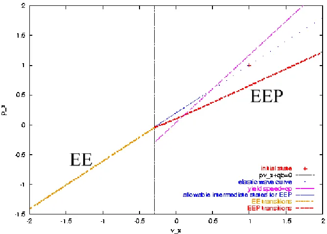
5.3 Wave Curves . . . 50
5.3.1 Characterizing Elastoplastic Transitions . . . 50
5.3.2 Characterizing the Hyperbola for Various (p, q) . . . 52
5.3.3 Constructing the Solution . . . 54
5.4 Comparison of Analytic and Numerical Results . . . 58
6 Periodic Solution 62 6.1 Introduction . . . 62
6.2 General Description . . . 63
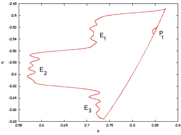
6.3 Phase plots . . . 66
6.3.1 Plottingp vs. q . . . 66
6.3.2 Phase Plots withw. . . 68
6.3.3 Long-time Phase Plots . . . 68
6.4 Effect of Parameter Values on the Periodic Solution . . . 71
6.4.1 Effect of Shear ModulusE . . . 71
6.4.2 Effect of Parameterα . . . 73
6.4.3 Effect of Mesh Size . . . 80
6.5 Bifurcation diagram . . . 81
7 Conclusion 83 7.1 Closing Remarks . . . 83
7.1.1 Hopper Flow . . . 83
7.1.2 Elastoplastic Transitions and Periodic Solution . . . 83
List of Figures
1.1 Block on Inclined Plane . . . 5
1.2 Coulomb yield locus,δ =π/20 . . . 6
2.1 Discretization of Elastoplastic Antiplane Shear Model . . . 13
2.2 The shear band solution of (2.1.17)–(2.1.18) . . . 14
2.3 Velocityvz=ax+by+w(x, t) of shear band solution in discretized antiplane shear model . . . 15
2.4 Location of τ (in (a)) with respect to ∇v (in (b)). . . 16
3.1 Hugoniot Locus of Hopper Flow in (σx, τ) space, from initial values σx ≈ 3.40, τ ≈0.19 . . . 24
3.2 Shock and characteristic speeds for steady hopper flow . . . 25
4.1 Stress (a) and ∇v(b) in antiplane shear, with ˆξ as defined in (4.1.6). . . 28
4.2 Form of F on each side of y=sx: increasing at zero on one side, decreasing at zero on other. . . 29
4.3 Example of Velocity and Stress in a Shear Band Equilibrium Soluion . . . . 30
4.4 Admissible (Dnsb, Dsb) for Shear Band . . . 32
5.1 Hyperbola of Elastoplastic Transitions . . . 47
5.2 Hyperbolas, depending on pand q . . . 53
5.3 Projection of the wave curve of states that can be connected to a left state (vL x, pLx, qxL) which satisfies (5.3.16). . . 56
5.4 Projection of the wave curve of states that can be connected to a left state (vxL, pLx, qxL) which does not satisfy (5.3.16). . . 58
5.5 Contour plots ofvx and kτk, showing the elastic and plastic regions, as well as a plastic wave on the left and an elastic wave on the right. . . 59
5.6 Contour plots of x-derivatives of p and q. . . . 60
5.7 Snapshots ofkτk and vx att=0, 0.2, 0.4, 0.6. . . . 60
5.8 Snapshots ofpx and qx att=0, 0.2, 0.4, 0.6. . . . 61
6.1 Contour Plot of w, N=40, E=0.1,α=π/4. . . . 63
6.4 Contour Plot of q, N=40, E=0.1,α=π/4 . . . . 65
6.5 Contour plot of kτk2, with regions labeled, N=40, E=0.1, α=π/4. . . . 65
6.6 Contour plot ofwover one period with regions labeled, N=40, E=0.1,α =π/4. 66 6.7 p versusq,x= 0.25,N = 40,E = 0.1,α=π/4 . . . . 67
6.8 p versusq,x= 0.475, N = 40, E= 0.1,α=π/4 . . . 68
6.9 p versusw,x=.25,N = 40, E= 0.1,α=π/4 . . . . 69
6.10 p versusw,x=.475, N = 40, E= 0.1,α =π/4 . . . . 69
6.11 p vs. q,x=.25, N = 40, E= 0.1, α=π/4, over many periods . . . . 70
6.12 Magnification of Figure 6.11 . . . 70
6.13 Phase plots ofpvs. q,N = 40, α=π/4. . . . 71
6.14 Phase plot ofp vs. w,N = 40, α=π/4. . . . 72
6.15 Dependence of period onE,N = 40, α=π/4. . . . 72
6.16 Contour ofkτk2,N = 40, E=.01,α=π/4. . . . 73
6.17 Contour ofw,N = 40,E =.1,α=π/4−.1. . . . 74
6.18 Contour ofkτk2,N = 40,E =.1,α=π/4−.1. The broad white space is at yield. . . 74
6.19 Phase plot ofp vs. q,N = 40, E= 0.1. . . 75
6.20 Change in the shape of the solution betweenα=π/4−.087 andα=π/4− .088,N = 40,E = 0.1. . . 75
6.21 Phase plot ofp vs. w,N = 40, E= 0.1. . . 76
6.22 Phase plot ofp vs. wfor lower values ofα,N = 40, E = 0.1. . . 77
6.23 Steady state shear band solution as a function ofα,N = 40,E = 0.1. . . . 77
6.24 Velocityw as a function of time for various α,N = 40,E = 0.1. . . 78
6.25 Velocitywas a function of time for various values ofx,α=π/4−.2,N = 40, E = 0.1. . . 79
6.26 Stress componentpas a function of time for various values ofx,α=π/4−.2, N = 40,E = 0.1. . . 79
6.27 Phase plots ofpvs. q,α=π/4, E= 0.033, N = 20,40,80,120. . . 80
6.28 Phase plots ofpvs. w,α=π/4,E= 0.033, N = 20,40,80,120. . . 81
Chapter 1
Introduction
The study of granular materials is at an exciting point, where mathematical anal-ysis can contribute to the understanding of a myriad of interesting phenomena. Recent experiments challenge traditional engineering theory, and there is still debate over phys-ical theories of granular flow [1], [3]. Mathematphys-ical analysis as well as numerphys-ical results may advance the process of winnowing out less applicable ideas and synthesizing those that remain.
The continuum models of steady state granular flow considered in this thesis are hyperbolic conservation laws (for many models, hyperbolicity can be lost, but we do not run into that issue here). Therefore, it is appropriate to consider the admissibility of shocks as weak solutions of the partial differential equations arising from these models.
Attempts to analyze the partial differential equations arising from the dynamics of granular flow models are complicated by the fact that these equations are dynamically ill-posed. In particular, they are unstable with respect to perturbations in certain directions in Fourier space [19]. Although in the linear theory, perturbations in these unstable direc-tions would lead to non-existence of soludirec-tions, nonlinear effects control the amplification of perturbations [20].
The model is thus a more analyzable system with the same key features as a full-blown granular flow model.
The numerical simulations in this thesis are results of spatial discretization of the equations of the antiplane shear model. If the partial differential equations governing antiplane shear are discretized in space, the ill-posedness is removed. Spatial discretization removes the effect of high frequency perturbations, arguably analogous to the effect that finite grain size has in the physical flow. Corresponding to the ill-posedness of the underlying continuum model, the discretized antiplane shear model can exhibit a sharp jump in the variables over one mesh width, representing a physical shear band.
Models of granular flow often assume plastic deformation; indeed, because the deformations in granular materials are primarily irreversible, they are excellent examples of ‘plastic’ materials [23]. Our model includes elasticity; we find it exhibits very complicated behavior, including a periodic solution for certain values of the shear modulus. This is particularly exciting because oscillatory behavior may contribute to hopper failure, and help explain the transition from mass flow to core flow. Thus, the elasticity of granular materials may play a greater role in their behavior than previously thought.
1.1
Phenomena in the Flow of Granular Materials
A granular material is any material composed of a large number of individual solid particles. Granular materials are ubiquitous in industry and agriculture. It is estimated that approximately one half of the products, and three quarters of the raw materials, of the chemical industry are in granular form [16]. When one considers the catastrophic power of avalanches, the economic significance of petroleum extraction, or the importance of grain storage from the dawn of civilization to the present, it becomes evident that predicting and controlling the behavior of granular materials is of critical importance. Despite this, our understanding of the behavior of granular materials is much less complete than that of fluids, for example. Our limited knowledge has a high price: in North America each year, over a thousand bins, hoppers, and silos fail, and the efficiency of industrial solids processing plants is poor [10].
as another form of matter entirely. For example, because the weight of grain in a silo is distributed to the walls, the pressure approaches a constant as the depth increases, rather than increasing linearly with depth like a liquid [9]. A similar effect is observed in granular material flowing from a hopper: the material can form arches, supporting the grains above it and arresting the outflow.
Granular material typically flows from a hopper in one of two modes: mass flow, which occurs for narrow hoppers and in which all the material is moving, and core flow, which occurs when the angle of the hopper is wider and in which stagnant regions of material form on the walls while a core of granular material near the center of the hopper continues to flow [16]. Stagnant regions are usually undesirable in practical applications, and demonstrate that granular flow is qualitatively different from fluid flow. In addition to these steady state flows, pulsating flow is often observed [19]. Hopper failure is thought to be the result of such oscillations, but this connection has not been studied in theory, analysis, or simulation.
One of the phenomena of granular flow demanding attention is the occurrence of localization of flow. Often, the displacement of a granular material is localized in a narrow band of material, called ashear band [23]. Because shear bands and associated phenomena (such as core flow) are so prevalent, it is critical that a granular flow model include solutions corresponding to shear bands.
1.2
Continuum Models of the Flow of Granular Materials
There are, in general, two approaches taken in modeling granular materials. One is to attempt to model the behavior of individual grains and their interactions with each other: these are referred to as molecular dynamic, micromechanical, or discrete element models. There is a broad literature on this topic, including attempts to simulate real deformations and flows [6], [14], [2], [11], [15].
1.2.1 Modeling Principles Force Balance
In a continuum with constant densityρ, conservation of momentum is represented by the formula
ρDv
Dt =ρf+∇ ·T, (1.2.1)
where f is a body force, such as gravity, Dv/Dtis the material derivative of velocity, and T is the stress tensor. Constitutive laws constraining the components of the stress tensor, and relating the stress components to velocity, are used to close the system. In the absence of body forces, steady state force balance is given by
∇ ·T =~0. (1.2.2)
The stress tensor is symmetric as a result of conservation of angular momentum. (A more complicated continuum model, taking into account the possibility of grains spinning relative to the grains surrounding them, is the Cosserat continuum model, which has an asymmetric stress tensor: see [23].) In two space dimensions, we denote the stress tensor by
T =
σx τxy
τxy σy
, (1.2.3)
whereτ is the shear stress; σx and σy are normal stresses in thexand ydirections, respec-tively.
In three space dimensions, the form of the stress tensor is
T =
σx τxy τxz τxy σy τyz τxz τyz σz
. (1.2.4)
Constitutive Laws
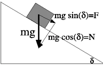
Figure 1.1: Block on Inclined Plane
threshold is analogous to the standard physics problem of a mass on an inclined plane (see Figure 1.1). If the coefficient of friction is µ, then the block moves if
F =µN, (1.2.5)
whereF is the tangential force down the slope, and N is the normal force. The angleδ at which this occurs is defined by the relationµ= tanδ.
In two dimensions, the analogy can be pursued further. For an idealized granular material, called a Coulomb material, the shear stressτ takes the role of F, and the normal stress σ that of N. The angle δ defined by µ= tanδ is called the angle of friction. Along every plane in the granular material, the following inequality holds:
τ ≤µσ =σtanδ. (1.2.6)
The granular material will flow plastically only if there is a plane along which equality is attained; this is the first constitutive law, theCoulomb yield condition. When the inequality is strict, the material behaves elastically, but this case is often ignored: in hopper flow, for example, it is generally assumed that all the material is flowing, although experimentally this is not always the case. There are competing generalizations of the Coulomb yield condition to three dimensions; the Tresca and von Mises conditions are commonly used [23], but we shall not consider them here.
0 2 4 6 8 10
sigma_y
–2 2
tau
2 4
6 8
10 sigma_x
Figure 1.2: Coulomb yield locus, δ=π/20
free-standing granular material forms this characteristic angle of steepness. Viewing Figure 1.1 as a slope of granular material, the link between the angle of repose and the Coulomb yield condition is clear; one can imagine the block as a grain, which will fall down the slope if the angle of the slope is δ or greater.
To derive the Coulomb yield condition, let us assume that the granular material is in a state of incipient flow everywhere; that is, at every point within the granular material, the inequality 1.2.6 achieves equality for some plane. By maximizing τ /σ over all planes through a point, and setting that ratio to tanδ, we obtain an algebraic constraint on the componentsσx,σy, and τxy:
µ
σx−σy 2
¶2
+τxy2 =
µ
σx+σy 2
¶2
sin2δ. (1.2.7)
This constraint is the Coulomb yield condition: it describes a cone in (σx, σy, τxy) space, as depicted in Figure 1.2.
Regardless of which yield condition is used in three dimensions, the steady state equations do not decouple, and another constitutive law is required to relate the velocity to the stress: such a relation is known as aflow rule. (A notable exception is 3-d axisymmetric granular flow, in which the circumferential shear stresses vanish, and an assumption about the circumferential normal stress can decouple the stress from the velocity [16].) A flow rule is also necessary to close the dynamic system (1.2.1). The flow rule relates stress and strain rate through the strain rate tensor,V:
V = 1
2(∇v+∇v
T). (1.2.8)
A typical flow rule is the associative or coaxial flow rule, which asserts that the eigenvectors of the stress tensor T and the strain rate tensor V are parallel. However, experimental results [23] indicate that a nonassociative flow rule, for which the eigenvectors ofT and V do not align, is more realistic.
Rankine states
The cone of Figure 1.2 indicates that in general, a value of σx and τ determines not one but two possible values ofσy. For each point along the axis of the cone, half of the circular cross-section of the cone hasσx≥σy while for the other half, the opposite inequality holds. These two halves of the cone are referred to as thepassive andactive Rankine states, respectively. If y signifies the vertical direction, the passive state reflects the behavior of a granular material that is being compressed horizontally more than it is being compressed vertically, such as might happen in a funnel or hopper. The active state is one for which the vertical stress is dominant, as one might expect in a free pile of granular material, or in a standpipe. Transitions between active and passive are expected in practical applications, such as a conical hopper atop a cylindrical standpipe; modeling such a transition is an open problem [5].
1.2.2 Ill-Posedness in Continuum Models
The equation (1.2.1) with an appropriate yield condition and the coaxial flow rule is dynamically ill-posed. The instability is analogous to the equation
tion. Thus, infinitesimal plane wave perturbations in a particular direction will be amplified, but the solution does not grow uncontrollably [19]. The instantaneous but finite amplifica-tion of infinitesimal perturbaamplifica-tions in unstable direcamplifica-tions in Fourier space is comparable to shear band formation, where a large (but not unbounded) displacement is concentrated in a narrow region.
1.3
Summary of Results
1.3.1 Shocks in Hopper Flow
We prove that in two-dimensional and three-dimensional axisymmetric steady state hopper flow, the Hugoniot locus, which describes possible stresses on either side of a dis-continuity, is a closed curve, topologically equivalent to a figure of eight, wrapping around the conical yield surface of Figure 1.2. Shocks between active and passive Rankine states, thought to be part of a solution for a funnel-standpipe combination, do not satisfy the Lax entropy condition.
1.3.2 Elastoplastic Antiplane Shear
1.3.3 Elastoplastic Transitions in Antiplane Shear
There is a surprising parallel with [21], where a continuous piecewise linear solution was constructed for piecewise linear initial data for a model of longitudinal displacement in an elastoplastic rod. The same approach can be applied to determine the local behavior of the elastoplastic antiplane shear problem with piecewise linear initial data. A piecewise linear initial condition is seen to generate elastic waves, elastoplastic transitions, and/or plastic waves, each propagating with a determinable speed. These waves resemble parts of the periodic solution that arises for low values of the shear modulus in elastoplastic antiplane shear.
1.3.4 Periodic Solution in Antiplane Shear
We use numerical simulations to systematically explore the effect of variation of the parameters of the antiplane shear problem on the solution. The parameters varied are the shear modulus E, which determines the elasticity of the granular material; the angle α, which determines the degree of nonassociativity of the system, and the mesh size of the spatial discretization, ∆x.
Chapter 2
Background
2.1
Antiplane Shear Model
2.1.1 Motivation and development of model
The antiplane shear model is simpler than a general continuum model of a granular material, while retaining the ill-posedness typical of these models. Thus, the antiplane shear model is unstable with respect to perturbations in a wedge of directions in Fourier space, but consists of only one velocity component and two stress components.
It presumes that all movement of the granular material is in one direction, which we take to be parallel to thez axis:
vx =vy = 0. (2.1.1)
In addition, the antiplane shear model assumes that there is no dependence of velocity or stress on z. Consequently,
v· ∇v=
0 0 vz
·
∂vz
∂x ∂vz
∂y
0
= 0, (2.1.2)
so the material time derivativeDv/Dt=∂v/∂t. These assumptions also eliminate most of the stress components from the momentum balance equation, leaving only the shear stresses τxz and τyz. Finally, the material is assumed to be incompressible (ρ is constant), so that (1.2.1) becomes
∂vz ∂t =
∂τxz ∂x +
∂τyz
For convenience of notation, we will rename vz as simply v (as the velocity is a scalar in this model), and the vector (τxz, τyz)T of shear stresses asτ, so that we can use subscripts to denote derivatives and (2.1.3) can be rewritten
vt=∇ ·τ. (2.1.4)
We need constitutive laws to close the system (which is now just one partial differential equation with three unknowns.)
The yield condition constrains the magnitude of the shear stresses:
kτk ≤1. (2.1.5)
The flow rule changes form depending on whether the material is deforming elasti-cally or plastielasti-cally. With the reduction in variables, the flow rule is no longer a relationship between tensors, but between the vectorsτ and∇v= (vx, vy)T. In elastic deformation, the
time derivative of stress is proportional to the spatial derivative of velocity:
τt=E∇v. (2.1.6)
In plastic deformation, the time derivative of stress must be such that the yield condition (2.1.5) is not violated. The flow rule
τt=E
µ
∇v−τ · ∇v
cosα R
T ατ
, (2.1.7)
whereRα is the rotation matrix ¡cossinαα−cossinαα¢, 0≤α < π/2, satisfies the yield condition: Lemma 1. If kτ(x,0)k ≤1 for all x, and τt is given by (2.1.7), then kτ(x, t)k ≤1 for all x at any t≥0.
Proof. We first observe that the time derivative of kτk is
kτkt=√τ·τt= (τ ·τt)/kτk, (2.1.8)
so τ ·τt has the same sign as kτkt. (We can safely ignore the case kτk = 0.) We assume without loss of generality that kτk= 1 at some point (x0, t0). Then
τ ·τt=τ ·E
µ
∇v−τ· ∇v
cosα R
T ατ
=E(τ· ∇v)(1− kτk2) = 0.
(2.1.9)
τt=E
µ
∇v−χ(kτk)(τ · ∇v)+
cosα R
T ατ
, (2.1.10)
where the transition from elastic to plastic is expressed by the indicator function χ:
χ(kτk) =
0 ifkτk<1 1 ifkτk ≥1.
(2.1.11)
The +-subscript in (2.1.10) indicates the positive part of the function: (τ·∇v)+= τ · ∇v ifτ · ∇v >0, and 0 otherwise. This expresses loading; if the material is at yield but is unloading (τ · ∇v≤0), the elastic flow rule applies.
A transition from the plastic to the elastic form of the equations can only occur through unloading:
Corollary 1. If τ evolves according to (2.1.10), and kτ(x, t)k ≥1and τ(x, t)· ∇v(x, t)>0 for some (x, t), then (2.1.10) will reduce to the elastic evolution equation (2.1.6) at (x, t∗) for some t∗ > t only ifτ(x, t∗)· ∇v(x, t∗)≤0.
Proof. As seen in (2.1.9), τ·τt= 0 ifkτk= 1 andτ· ∇v >0, and thereforekτkwill remain at 1 untilτ · ∇v≤0.
Thus, plastic to elastic transitions are characterized byτ · ∇v becoming negative. On the other hand, for the elastic or unloading states (kτk < 1 or τ · ∇v ≤ 0), τ ·τt = E(τ · ∇v), so unloading states have decreasing kτk, while for loading elastic states, kτk increases untilkτk= 1. Thus, a transition from elastic to plastic occurs whenkτkbecomes 1 (the elastic state must be loading for kτkto increase, so τ · ∇v >0 already).
2.1.2 One-Dimensional Model
A linear functionv=ax+bycoupled with a constantτ =Rα∇v/k∇vkis a steady state solution of the equations (2.1.4) and (2.1.10):
vt=∇ ·τ =∇ ·
Rα
a
b
/(a2+b2)
= 0 (2.1.12)
τt=E
µ
∇v− τ· ∇v
cosα ∇v/k∇vk
=E
µ
∇v−k∇vk∇v
k∇vk
w
w
w
w
w
τ
τ
τ
τ
0
1
w
Ν−1
Ν
0
0
1
Ν−1
2
=
2
. . .
. . .
Figure 2.1: Discretization of Elastoplastic Antiplane Shear Model
The material is plastic for all x, and loading because of the constraint α < π/4. This solution represents a uniform shear, and might represent a solution for the system (2.1.4), (2.1.10) on the domain {x ∈ [0,1];y ∈R;t > 0} with boundary conditions v(0, y, t) = by, v(1, y, t) =a+by, for example, as in [25].
We introduce a perturbation w(x, t) in time and only one space dimension of this uniform shear: v = ax+by+w(x, t). Without loss of generality, we also normalize a2+b2= 1. Relabeling the components of τ =
³
p(x,t) q(x,t)
´
, the equations of motion become
wt=∇ ·τ =px, (2.1.14)
τt=E
a+wx
b
−
χ(kτk)
τ·
a+wx
b +
cosα R
T ατ , (2.1.15)
with the same yield condition, expressed by the indicator functionχ(kτk) defined in (2.1.11). We observe that the equations are unchanged if a constant is added tow.
Spatial Discretization
-0.8 -0.6 -0.4 -0.2 0 0.2 0.4 0.6
0 0.2 0.4 0.6 0.8 1 x
w
p
q
Figure 2.2: The shear band solution of (2.1.17)–(2.1.18)
If we define a difference operator by
Dn(f(x)) = (fn−fn−1)/∆x, (2.1.16)
the discretized form of (2.1.14)–(2.1.15) is
dwn
dt =Dn(p) (2.1.17)
dτn dt =E
a+Dn+1(w)
b
−χ(kτnk) (pn(a+Dn+1(wn)) +qnb)+
cosα R
T ατn
(2.1.18)
forn= 0, . . . , N−1.
Applying periodic boundary conditions introduces the constraints wN =w0,τN = τ0. Since adding a constant to w does not change (2.1.17)–(2.1.18), periodic boundary conditions are equivalent to Dirichlet conditions onw.
2.1.3 Shear Band Solution
Figure 2.3: Velocity vz =ax+by+w(x, t) of shear band solution in discretized antiplane shear model
perturbationwmakes a large jump, as shown in Figure 2.2. The velocityv=ax+by+w(x, t) (and therefore displacement) exhibits a sudden jump along a particular value of x, much like a physical shear band; see Figure 2.3.
Because of the periodic boundary conditions, the location of this shear band is undetermined. (In practice, the location of the shear band will be determined by the initial conditions of the dynamic problem.) These shear band solutions are entirely plastic (that is,kτnk= 1 andτn·(a+Dn(w), b)T ≥0 for alln).
As shown in equation (2.1.13), the expression τ = Rα(∇v)/k∇vk satisfies the steady state form of (2.1.15). In the same manner, the expression
τn= Rα
a+Dn+1(w)
b
p
(a+Dn+1(w))2+b2 (2.1.19) satisfies (2.1.18), the discretized form of (2.1.15). The steady state form of (2.1.17),Dn(p) = 0, simply asserts thatp must be constant in an equilibrium solution.
Figure 2.4: Location ofτ (in (a)) with respect to ∇v (in (b)).
there is an angle θ such that pn = cosθ, and qn = ±sinθ for all n. Each of these states corresponds to a single value of∇vn= (a+Dn(w), b)T, since the vectorτnis a fixed rotation of the unit vector ∇v/k∇vk; see Figure 2.4. We restrict θ to the range
0≤θ≤π/2, (2.1.20)
which is the case depicted in Figure 2.4, appropriate if the underlying uniform shear satisfies b < 0. (There is a symmetric case for uniform shears with b > 0, for which π/2 ≤ θ ≤ π. Hereafter we assume the case b < 0.) The values of variables at the shear band are subscripted “sb”, while those for all other n are subscripted “nsb”. As can be seen in Figure 2.4, solutions of this type must satisfy
θ−α <0, (2.1.21)
in order to meet the condition [∇vsb]2 =b <0.
Whether a given angleθ < αgenerates an equilibrium solution depends on whether it satisfies the boundary conditions. In order to satisfy the boundary condition wN =w0, the sum overn of theDn(w) must be zero. This is an algebraic relation betweenDn(w)sb and Dn(w)nsb:
In Figure 2.4, the coordinates of ∇vnsb and∇vsb are given by
∇vsb =
a+Dn(w)sb
b
=
bcot(θ−α)
b
, (2.1.23)
∇vnsb =
a+Dn(w)nsb
b
=
−bcot(θ+α)
b
. (2.1.24)
Therefore, the boundary condition (2.1.22) can be written in terms ofθ as
(bcot(θ−α)−a) + (N −1)(−bcot(θ+α)−a) = 0. (2.1.25)
Thus,
∆xcot(θ−α)−(1−∆x) cot(θ+α) =a/b. (2.1.26)
We seek a solution θ to (2.1.26). As ∆x → 0, Dn(w)sb → ∞, so (2.1.23) indicates that θ→α. In [22], a formula for θis obtained to first order in ∆x, rewritten here as
θ=α+ 1
cotφ+ cot 2α∆x, (2.1.27)
in which the angle φis defined by
(a, b) = (cosφ,sinφ). (2.1.28)
Uniqueness of the solution to (2.1.26) will be analyzed further in Chapter 4, but for typical values ofα and φ, (2.1.26) has a unique solution forθ.
2.1.4 Periodic Solution
The shear band solution is stable for suitably high values of the shear modulus E > Ecrit [22]. In terms ofθ,
Ecrit≈ 8 sin
2(α−θ) sin(θ) cos(α) sin(θ+α)
b2∆x . (2.1.29)
Thus, as ∆x→ ∞, using (2.1.27) and (2.1.28) we expressEcrit as
Ecrit= 4 sin
22α
cos2φ+ sin 2φcot 2α+ cot22α∆x+O(∆x
2). (2.1.30)
For example, forα=π/4, (2.1.30) reduces to
Ecrit = 4∆x
thanEcrit, a periodic solution develops, in which the shear band changes its strength over time, and for some values ofα, disappears entirely for part of the period [22]. This periodic solution is described and analyzed extensively in Chapter 6.
2.2
Plastic Antiplane Shear Model
2.2.1 Description of the Plastic Model
The plastic antiplane shear model is the limit of the elastoplastic system as the shear modulus E goes to infinity. In order for τt to remain bounded in (2.1.10), the factor
∇v−χ(kτk)(τ· ∇v)+
cosα R
T
ατ →0, (2.2.1)
which, as seen in (2.1.13), occurs if
τ =Rα ∇v
k∇vk. (2.2.2)
With an explicit representation forτ, the system reduces to a partial differential equation in the one variable v:
vt=∇ ·τ =∇ ·Rα ∇v
k∇vk. (2.2.3)
2.2.2 One-Dimensional Plastic Model
As in the elastoplastic case, we observe that a linear function v = ax+by is a steady state solution of the equation (2.2.3):
vt=∇ · Rα a b √
a2+b2 =
∇ ·
acosα−bsinα
asinα+bcosα
√
a2+b2 = 0. (2.2.4)
We again introduce a perturbation w(x, t) to this uniform shear, in which case (2.2.3) reduces to
wt=∇ · Rα
a+wx
b
p
(a+wx)2+b2 =∂x
Ã
(a+wx) cosα−bsinα
p
(a+wx)2+b2
!
. (2.2.5)
satisfying Dirichlet boundary conditions is ill-posed to perturbations, demonstrating that the model still retains the ill-posedness typical of granular flow models [25]. (For other ranges of parameters, the trivial solution is stable, and initial data satisfying a bound on the upper value ofwx converges to the trivial solution ast→ ∞.)
2.2.3 Shear Bands
Using the same difference operator defined by (2.1.16), the discretization of (2.2.5) is
dwn dt =
1 ∆x
Ã
(a+Dn+1(w)) cosα−bsinα
p
(a+Dn+1(w))2+b2 −
(a+Dn(w)) cosα−bsinα
p
(a+Dn(w))2+b2
!
. (2.2.6)
The shear band solutions to the discretized elastoplastic antiplane shear model, found in Subsection 2.1.3, are entirely plastic solutions. It is perhaps not surprising then that these shear band solutions are also solutions of the plastic model.
2.3
Solutions to Riemann-type Problems in Elastoplastic Model
of Longitudinal Displacement in a Rod
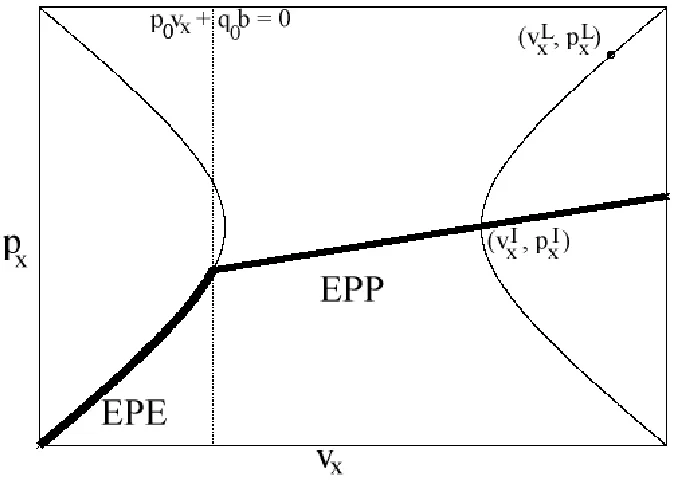
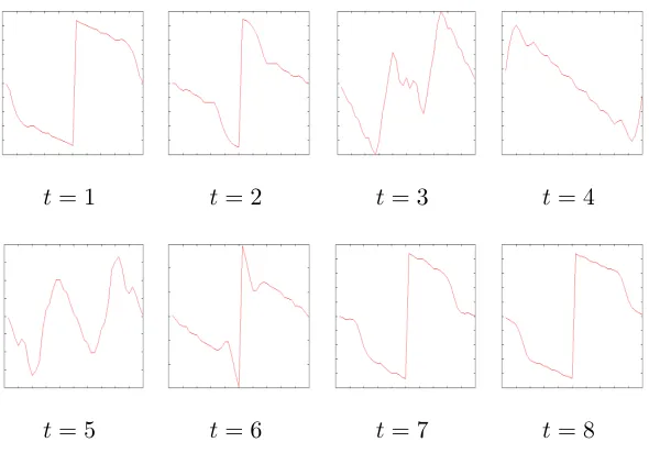
The periodic solution described in 2.1.4 consists of nearly linear sections separated by sharp transitions, which propagate through the domain; see Figure 6.1. The form of the periodic solution prompts the investigation of propagating transitions in the equations of elastoplastic antiplane shear.
vt=σx, σt+kγt=vx,
γt=
0 ifσ < γ (elastic) (σt)+ ifσ=γ (plastic).
(2.3.1)
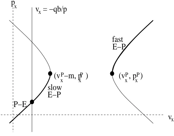
Consider continuous solutions with discontinuous x-derivatives of the “SI prob-lem”, specifically (2.3.1) with the initial conditions
v(x,0) =
aLxforx≤0 aRxforx≥0
σ(x,0) =
bLx forx≤0 bRx forx≥0
γ(x,0) =
cLx forx≤0 cRx forx≥0.
(2.3.2)
This problem is scale invariant, meaning that the equations and initial conditions are unchanged under the scaling
˜
v(x, t) =η−1v(ηx, ηt), σ(x, t) =˜ η−1σ(ηx, ηt), γ(x, t) =˜ η−1γ(ηx, ηt). (2.3.3)
Scale invariant solutions U = (v(x, t), σ(x, t), γ(x, t))T take the form U(x, t) = tF(x/t). From this it follows that, between characteristics, the solution in a wedge of either plastic or elastic deformation is in fact linear: U(x, t) = xU0 +tU1. In addition, the form of U determines that any transition from elastic to plastic (or vice versa) occurs along a radial line.
γ, so γx may jump along x = 0. On the other hand, if the line x = 0 is in a plastic state, then γx =σx; continuity of σx implies the continuity of γx. Therefore, a continuous solution to (2.3.1)–(2.3.2) can be constructed by choosing the transitions corresponding to the intersection point of the aforementioned loci of (vx, σx) alongx= 0.
Chapter 3
Shocks in Steady Hopper Flow
3.1
Hugoniot locus
3.1.1 2-d Hopper Flow
We restate the Coulomb yield condition (1.2.7) for convenience:
µ
σx−σy 2
¶2
+τxy2 =
µ
σx+σy 2
¶2
sin2δ. (3.1.1)
As shown in Figure 1.2, the yield condition (3.1.1) describes a cone.
The steady state momentum balance equation (1.2.2) in two dimensions is
∂x
σx
τxy
+∂y
τxy
σy
=
g
0
, (3.1.2)
where g is acceleration due to gravity and x is the downward vertical direction. This system can be viewed as a system of conservation laws, with x playing the role of time. The Rankine-Hugoniot condition for such a system, using square brackets to denote jumps across a discontinuity interface x=sy would be
[τxy] =s[σx] (3.1.3)
[σy] =s[τxy]. (3.1.4)
Where the brackets denote the jump across the discontinuity:
[f(x, y)] = lim
Eliminatingsfrom (3.1.3)–(3.1.4), we have the Hugoniot locus
[σx][σy] = [τxy]2. (3.1.6)
Equation (3.1.6) relates six unknowns, the values of (σx, σy, τxy) on each side of the discon-tinuity. If the stress components are specified on one side of the discontinuity, the equation of the Hugoniot locus (3.1.6) also describes a cone; the intersection of the cones (3.1.1) and (3.1.6) is the locus of possible states on the other side of the discontinuity satisfying the yield condition.
Theorem. Suppose the stress components(σL
x, σLy, τxyL) are fixed on one side of the
discon-tinuityx=sy, satisfying the yield condition (3.1.1) withδ < π/2. Then the Hugoniot locus (3.1.6) is a closed curve, topologically equivalent to a figure-of-eight.
Proof. The cone (3.1.1) has axis σx =σy, τxy = 0, with opening angleβ, whereβ satisfies the equation tanβ = sinδ. Forδ < π/2, tanβ <1 and therefore β < π/4..
On the other hand, the cone (3.1.6) can be written
µ
[σx]−[σy] 2
¶2
+ [τxy]2 =
µ
[σx] + [σy] 2
¶2
. (3.1.7)
Therefore, this cone has a parallel axis to (3.1.1), although its vertex has been shifted to (σLx, σyL, τxyL). The opening angle is π/4.
The intersection between two cones of different opening angle is nontrivial. How-ever, we can demonstrate that this intersection is contained within a parabolic cylinder.
First we simplify by denoting
ξ = σx−σy
2 (3.1.8)
ν = σx+σy
2 (3.1.9)
ξL= σ
L x −σyL
2 (3.1.10)
νL= σ
L x +σyL
2 . (3.1.11)
Then, the cones (3.1.1) and (3.1.6) are
–0.8 –0.6 –0.4 –0.2 0 0.2 0.4
3 3.5 4 4.5 5 5.5 6
Figure 3.1: Hugoniot Locus of Hopper Flow in (σx, τ) space, from initial values σx ≈ 3.40, τ ≈0.19
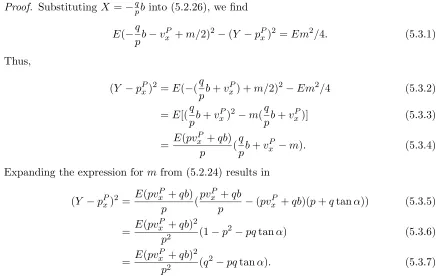
Expanding (3.1.13) and applying (3.1.12) gives
−ξξL−τxyτxyL +ννL= (ν2+ (νL)2) cos2δ/2. (3.1.14)
This is a parabolic cylinder, rewritable as
ξξL+τxyτxyL =−cos
2δ
2
µ
ν− ν
L
cos2δ
¶2
+(v
L)2
2
µ
1
cos2δ −cos
2δ¶. (3.1.15)
The axis of the parabolic cylinder (3.1.15) is the planeν=νL/cos2δ, which is perpendicular to the axes of both cones (which are the ν-axis and the line parallel to it (ξ = ξL, τ
xy =
τxyL, ν ∈R). Therefore the parabolic cylinder cuts through the cones. The projection of the yield cone (3.1.12) onto the (ξξL+τxyτxyL, ν) plane is
ξξL+τxyτxyL =ν2sin2δ. (3.1.16)
The projection of the Hugoniot locus into (σx, τxy) space is shown in Figure 3.1. The yield condition constrainsσy to a cone, which results in the locus looping back on itself. Most important is determining if there are Lax shocks which permit a transition from passive to active state (that is, from the top of the cone to the bottom.)
3.2
Shock speeds
Figure 3.2: Speed of shock given by Rankine-Hugoniot condition (green), characteristic speeds (red, blue), as functions of the angleψ around the yield cone.
on each side of the shock [12]. For hopper flow, the speeds of the characteristics are given by
λ±= tan
³
ψ±π 4
´
, (3.2.1)
where ψ is half the angle around the yield cone (ψ = 0 is the extreme of the passive case, the highest point on the cone in Figure 1.2.) The results are shown in Figure 3.2. The asymptotes for the characteristic speeds lie at ψ = ±π/4, the boundary between passive and active states. As a result, the Lax shocks (those for whichλL+ > s+> λR+, and similarly for the minus branch) from a left state in the passive region have a right state in the passive region as well: there are no Lax shocks between passive and active states.
Chapter 4
Antiplane Shear
4.1
Instability of Piecewise Linear Solutions in Plastic
An-tiplane Shear
Consider the plastic antiplane shear model (2.2.3):
vt=∇ ·τ, τ =Rα ∇v
k∇vk. (4.1.1)
In Subsection 2.2.2, it was shown that a uniform shear v = ax+by satisfies (4.1.1). We went on to introduce a one-dimensional perturbation to the uniform shear, discretized in space, and found shear band solutions to the discretized problem.
Another approach is to consider solutions of (4.1.1) with continuous velocity but a discontinuity in the stressτ along a liney=sx. We take vs to be piecewise linear:
vs=
aLx+bLy, y > sx aRx+bRy, y < sx
. (4.1.2)
We treat x as timelike, and q as a function of p, so that px +qy = 0 has the form of a conservation law. The Rankine-Hugoniot condition is
s= [q]
[p], (4.1.3)
Theorem. Suppose vs(x, y), as defined in (4.1.2), is a solution of (4.1.1)satisfying (4.1.3). Then this solution is unstable with respect to a perturbation in time and one space dimension w(y−sx, t).
Proof. Let v=vs+w(y−sx, t). Then the dynamic equation (4.1.1) is
∂tv=∇ ·
µ
Rα ∇v
k∇vk
. (4.1.4)
The perturbationw(y−sx, t) is one dimensional in space, perpendicular to the fronty=sx. We define the variableξ to represent the distance from the discontinuity:
ξ =y−sx, (4.1.5)
and the unit vector perpendicular to the discontinuity
ˆ
ξ=∇ξ/k∇ξk= √(−s,1)
1 +s2. (4.1.6)
Then (4.1.4) can be written as
∂tw=∂ξ
Ã
Rα ∇vs+ (∂ξw) ˆξ
k∇vs+ (∂ξw) ˆξk· ˆ ξ
!
. (4.1.7)
This can be abbreviated as
∂tw=∂ξ(F(∂ξw)), (4.1.8)
where
F(u) =
Ã
Rα ∇vs+u ˆ ξ
k∇vs+uξˆk · ˆ ξ
!
. (4.1.9)
Letu=∂ξw, and apply ∂ξ to both sides of (4.1.8):
∂tu=∂ξ¡F0(u)∂ξu¢. (4.1.10)
Equation (4.1.10) is a diffusion equation; if F0(u) > 0, it behaves like the heat equation, but ifF0(u)<0, then (4.1.10) is unstable, like the backwards heat equation.
ξ
^
v
(a) (b)
stress =(p,q)τ
ξ
^
(a ,b )
B B
umax< 0 max> 0
u R ξ^
T α τ τ A B [q] [p]
(a ,b )
A A
Figure 4.1: Stress (a) and∇v (b) in antiplane shear, with ˆξ as defined in (4.1.6).
The maximum ofF(u) can be seen by inspection of (4.1.9) to occur atumax, where
∇vs+umaxξˆ
k∇vs+umaxξˆk =R
T
αξ.ˆ (4.1.11)
In Figure 4.1(b), we see that since ˆξ bisects the two stresses, RTαξˆbisects the two velocity gradients. Therefore, the value ofumaxon each side of the discontinuity has a different sign. The structure ofF (given by (4.1.9)) is such thatF is increasing foru < umax and decreasing for u > umax; see Figure 4.2. Since umax switches sign across the discontinuity, F is increasing atu= 0 on one side of the shock, but is decreasing on the other side of the front. Therefore, the solution is unstable on one side of the front with respect to arbitrarily small perturbationsw.
4.2
Shear Band Solution of Spatially Discretized Antiplane
Shear
We now quantify the shear band solution described in 2.1.3. Recall the discretized form of the antiplane shear problem, (2.2.6), rewritten here as
dwn dt =
1 ∆x
·
Rα ∇n+1v
k∇n+1vk−
Rα ∇nv
k∇nvk
¸
1
F(u), on side “A” of the discontinuity
F(u), on side “B” of the discontinuity
Figure 4.2: Form of F on each side ofy =sx: increasing at zero on one side, decreasing at zero on other.
where∇nv= (a+Dn(w), b)T. Sincea2+b2 = 1, we define the angleφby (2.1.28), restated here:
a= cosφ, b= sinφ. (4.2.2)
Consider a shear band solution to (4.2.1) under a periodic boundary condition:
w0 =wN. (4.2.3)
Such a solution is identified by two values of Dn(w) = (wn−wn−1)/∆x: the difference operatorDn(w) takes the valueDnsb for all values ofnexcept one, for whichDn(w) =Dsb. Note that the position of the shear band (the value of n for which Dn(w) = Dsb(w)) is undetermined.
We proceed to determine conditions on the parameters (α, φ, N) so that a shear band solution exists, and determine how many such shear band solutions there are for a given set of parameters.
As in 2.1.3, only solutions with a single jump in velocity are considered. Recall thatα is chosen in the range
0≤α≤π/2. (4.2.4)
We assume the angleφof the underlying uniform shear is constrained so thatb= sinφ <0 (cf. the discussion in Subsection 2.1.3; the case b > 0 generates a symmetric result). We further constrainφto the range
−π/2≤φ <0, (4.2.5)
vnsb vnsb vnsb vnsb vnsb vsb vsb vsb R
τ =sb
vnsb vnsb
α
R
τ =nsb
Dnsb (a,b)= (cos , sin )φ φ vsb
Dsb vsb vsb α φ α α (a’,b’)
Figure 4.3: Example of Velocity and Stress in a Shear Band Equilibrium Solution. Given the underlying shearv0 =ax+byand the two values (Dnsb, Dsb) of the difference operator Dn(w), the velocity gradients are given by∇vnsb = (a+Dnsb, b), ∇vsb = (a+Dsb, b). If the associated stresses (τnsb =Rα ∇vnsb
k∇vnsbk, τsb =Rα ∇vsb
k∇vsbk) have the same first coordinate,
then these values of (Dnsb, Dsb) give a steady state solution of (4.2.1).
corresponding stress vectors (τnsb, τsb) for a shear band solution with parameters satisfying (4.2.4) and (4.2.5). Note that the point (a0, b0) represents a underlying uniform shear in the case −π ≤φ <−π/2; that choice ofφ would result in the same shear band solution, with the length of the chord between (a0, b0) and (a, b) added to both Dnsb and Dsb.
Theorem. Let (α, φ, N) be a parameter set satisfying (4.2.4), (4.2.5), and N >2. Then: 1. if −α < φ, then there are two pairs (Dnsb, Dsb) corresponding to steady state shear
band solutions of (4.2.1) and (4.2.3); these pairs are in quadrants II and IV.
2. ifφ <−2α, then there are no steady state shear band solutions of (4.2.1) and (4.2.3).
3. if−2α < φ <−α, the number of solutions depends on N; for each (α, φ), there exists a value Ncrit such that for N < Ncrit, there are no steady state shear band solutions; for N =Ncrit, there is exactly one shear band solution, and forN > Ncrit, there are two shear band solutions. For all these solutions, the pair (Dnsb, Dsb) is in quadrant IV.
Proof. A periodic boundary condition gives
wN −w0=
N
X
n=0
therefore
Dsb =−(N−1)Dnsb. (4.2.7)
Thus,Dsb is given in terms ofDnsb.
On the other hand, the steady state condition dwn
dt = 0 implies that the first
coordinate ofRα(∇nv/k∇nvk) is constant for alln. Given a value forDnsb, we can compute Rα(∇nsbv/k∇nsbvk), determine the other unit vector with the same first coordinate, and scale this to solve for Dsb. This process is immensely simplified by separating ∇nsbv into the components
∇nsbv=
a
b
+Dnsb
1 0 =
cosφ
sinφ
+Dnsb
1
0
. (4.2.8)
Then the stress vector τnsb is
τnsb =Rα(∇nsbv)/k∇nsbvk= 1
k∇nsbvk
cos(φ+α)
sin(φ+α)
+Dnsb
cosα
sinα
. (4.2.9)
As illustrated in Figure 4.3, the stress vector τsb is the reflection of τnsb around thex-axis. This is simply
τsb= 1
k∇nsbvk
cos(−(φ+α))
sin(−(φ+α))
+Dnsb
cos(−α)
sin(−α)
. (4.2.10)
To recover∇sbv/k∇sbvk,τsb is rotated counterclockwise byα:
∇sbv/k∇sbvk= k∇1 nsbvk
cos(−(φ+ 2α))
sin(−(φ+ 2α))
+Dnsb
cos(−2α)
sin(−2α)
(4.2.11)
∇sbv= k∇k∇sbvk nsbvk
cos(−(φ+ 2α))
sin(−(φ+ 2α))
+Dnsb
cos(−2α)
sin(−2α)
. (4.2.12)
They-component of∇sbvisb= sinφ(as seen in Figure 4.3). Therefore, the unknown ratio
k∇sbvk/k∇nsbvkin (4.2.12) can be solved for in terms ofφand α: k∇sbvk
k∇nsbvk =
sinφ
sin(−(φ+ 2α)) +Dnsbsin(−2α). (4.2.13) The x-component of ∇sbv is cosφ+Dsb. Thus, (4.2.12) and (4.2.13) give that
Dsb=−cosφ−sinφcos(φ+ 2α) +Dnsbcos(2α)
sin(φ+ 2α) +Dnsbsin(2α), or (4.2.14)
µ
Dsb+sin(φ+ 2α) sin(2α)
¶ µ
Dnsb+sin(φ+ 2α) sin(2α)
= sin
2φ
0 1 2 3 4 5 6 7
-0.8 -0.6 -0.4 -0.2 0 0.2
D_sb
D_nsb
boundary condition (N=10)
Figure 4.4: Admissible (Dnsb, Dsb) for Shear Band Solutions. The parameters areα=π/4, φ=−π/8, N = 10.
The equation (4.2.15) describes a hyperbola of slope pairs (Dnsb, Dsb) satisfying the condition dwn
dt = 0. If this pair also satisfies (4.2.7), then the boundary condition
w0 = wN is also satisfied. Thus, given the parameters (α, φ, N), the possible shear band solutions are characterized by the intersection points of the line (4.2.7) with the hyperbola (4.2.15), as seen in Figure 4.4.
The vertex of the hyperbola is
Dnsb =Dsb=−sinφ+ sin(φ+ 2α)
sin(2α) . (4.2.16)
The linear constraint (4.2.7) passes through the second and fourth quadrants, so all admis-sible pairs will be in one of those quadrants. If the vertex (4.2.16) is in the third quadrant, then there are necessarily exactly two intersection points of the line and hyperbola. The vertex (4.2.16) is 0 whenφ=−α. For the range
−α < φ <0, (4.2.17)
the vertex (4.2.16) is negative, so there are two intersection points, one with Dnsb < 0, Dsb>0, and the other with the signs reversed. This is case 1.
The asymptotes of the hyperbola (4.2.15) are
Dnsb =−sin(φ+ 2α)
sin(2α) and Dsb =−
sin(φ+ 2α)
If
φ <−2α, (4.2.19)
then the right-hand side of the asymptotes is positive, and the hyperbola is contained in the first quadrant, so it does not intersect the line (4.2.7), and there are no shear band solutions. This is case 2.
Finally, in the intermediate case
−2α < φ <−α, (4.2.20)
the vertex of the hyperbola is in the first quadrant, but the asymptotes are negative. For suitably large N, the line (4.2.7) will intersect the hyperbola (4.2.15) twice, while for N suitably near 2, the line will not intersect the hyperbola at all. (The slope of the line tangent to the hyperbola at the vertex is -1, which is the slope of the line (4.2.7) if N = 2. If the vertex is in the first quadrant, it is clear that the line (4.2.7) withN = 2 will not intersect it.) Between the two extremes is a value of N so that the line (4.2.7) is tangent to the hyperbola (4.2.15) at some point in the second quadrant; this is Ncrit, and completes the third case.
Although there are cases in Theorem 4.2 where two shear band solutions satisfy the boundary condition, only one such solution is seen in numerical simulations, because only the solution in the second quadrant (Dnsb <0, Dsb >0) with the largest value of Dsb is stable [25]. It is also interesting to consider the limit of the two pairs (Dnsb, Dsb) as N → ∞ (for cases 1 and 3). The stable solution approaches a discontinuity, with
Dnsb → −sin(φ+ 2α)
sin(2α) , Dsb → ∞, (4.2.21)
while the unstable solution approaches a constantw, a trivial perturbation:
Dnsb →0, Dsb→ sin
2(φ)−sin2(φ+ 2α)
sin(2α) sin(φ+ 2α) . (4.2.22)
4.3
Numerical Implementation of Elastoplastic Antiplane Shear
4.3.1 Enforcing the Yield Condition kτk ≤1.
results inkτk>1, ensuing steps will not increase kτk any further:
Corollary 2. kτkt>0 if and only if kτk<1 and τ· ∇v >0.
Proof. Equation (2.1.8) demonstrates that the sign of kτkt is the same as that of τ·τt. If τ · ∇v >0 (loading) andkτk ≥1 (plastic), (2.1.9) expresses τ·τt as
τ ·τt=E(τ· ∇v)(1− kτk2). (4.3.1)
Thus, ifkτk>1 andτ · ∇v >0,τ·τt<0, and thereforekτkt<0 also. On the other hand, ifτ · ∇v <0, then (2.1.6) gives that
τ·τt=E(τ · ∇v)<0. (4.3.2)
Thus, only whenτ· ∇v >0 andkτk<1, that is, the case of elastic loading, is kτkt>0.
This approach is not as stable as desired; very small timesteps (on the order of three or more orders of magnitude less than the space discretization size) are required to obtain results for which noise does not overwhelm the system [24].
Another approach is to enforce the yield locus, so that if any step results inkτk>1, τ is renormalized so thatkτk= 1. Such a case should result in the plastic state, since the yield locus has been reached. Unfortunately, machine arithmetic may compute the norm of the renormalizedτ as less than 1, and the elastic form of the equations would be incorrectly applied. This miscalculation can be avoided by setting a flag variable, so that the plastic form of the equations is always used immediately after a renormalization. This approach results in greater stability than depending on Corollary 2. Another approach to avoiding the renormalization error in machine arithmetic would be to renormalizeτ so thatkτk= 1 +², with²one order of magnitude larger than machine error.