Transition Densities and Sample Frequency Spectra of Diffusion Processes with Selection and Variable Population Size

GENETICS | INVESTIGATION

Transition Densities and Sample Frequency Spectra

of Diffusion Processes with Selection and Variable

Population Size

DanielZivkovi´c,*ˇ ,1_{Matthias Steinrücken,}†,‡_{Yun S. Song,}†,§_{and Wolfgang Stephan*}

*Section of Evolutionary Biology, Department of Biology, Ludwig-Maximilian University Munich, 82152 Munich, Germany, †_{Department of Statistics and}§_{Computer Science Division and Department of Integrative Biology, University of California, Berkeley,}

California 94720, and‡Department of Biostatistics and Epidemiology, University of Massachusetts, Amherst, Massachusetts 01003

ABSTRACT Advances in empirical population genetics have made apparent the need for models that simultaneously account for selection and demography. To address this need, we here study the Wright–Fisher diffusion under selection and variable effective population size. In the case of genic selection and piecewise-constant effective population sizes, we obtain the transition density by extending a recently developed method for computing an accurate spectral representation for a constant population size. Utilizing this extension, we show how to compute the sample frequency spectrum in the presence of genic selection and an arbitrary number of instantaneous changes in the effective population size. We also develop an alternate, efficient algorithm for computing the sample frequency spectrum using a moment-based approach. We apply these methods to answer the following questions: If neutrality is incorrectly assumed when there is selection, what effects does it have on demographic parameter estimation? Can the impact of negative selection be observed in populations that undergo strong exponential growth?

KEYWORDSdemography; diffusion; frequency spectrum; selection; transition density

A

DVANCES in empirical population genetics have pointed out the need for models that simultaneously account for selection and demography. Studies on samples from various species including humans (e.g., Williamson et al. 2005; Tennessen et al. 2012) and Drosophila melanogaster (Glinka et al.2003; Duchenet al.2013) have shown that demographic processes, such as population size changes, shape in large part the patterns of polymorphism among genomes and estimated the impact of selection on top of such underlying neutral con-ditions. Thus far, most theoretical articles considered selective and demographic forces independently of each other for the sake of simplicity (e.g., Stephan and Li 2007).

Theoretical studies of neutral models of time-varying population size have been accomplished within the diffusion and the coalescent frameworks. Kimura (1955a) derived the transition density of the Wright–Fisher (WF) diffusion with a constant population size that characterizes the neutral evolution of allele frequencies over time. Shortly thereafter,

Kimura (1955b) noted how to rescale time to generalize this result to a deterministically changing population size. Nei et al. (1975) derived the average heterozygosity under this general condition by applying a differential equation method, before studies on time-varying population size started to utilize the coalescent. Watterson (1984) derived the probability dis-tribution and the moments of the total number of alleles in a sample using models of one or two sudden changes in population size. Slatkin and Hudson (1991) considered the distribution of pairwise differences in exponentially growing populations, before Griffiths and Tavaré (1994) provided the coalescent for arbitrary deterministic changes in population size. The allele frequency spectrum, which is the distribution of the number of times a mu-tant allele is observed in a sample of DNA sequences, has been utilized in many theoretical and empirical studies. It can be fur-ther distinguished into the allelic spectrum and the sample fre-quency spectrum (SFS) according to whether absolute or relative frequencies are meant. Fu (1995) derived thefirst- and second-order moments of the allelic spectrum for a constant population size, which has been generalized to time-varying population size by Griffiths and Tavaré (1998) andZivkovi´c and Wiehe (2008).ˇ Although deterministic fluctuations in population size are commonly considered for the interpretation of biological Copyright © 2015 by the Genetics Society of America

doi: 10.1534/genetics.115.175265

Manuscript received January 29, 2015; accepted for publication April 9, 2015; published Early Online April 14, 2015.

1_{Corresponding author: Section of Evolutionary Biology, Department of Biology,}

data, studies have also examined stochastic changes in population size (e.g., Kaj and Krone 2003).

The mathematical modeling of natural selection is mostly carried out within the diffusion framework, whereas coalescent approaches have proved to be analytically challenging (e.g., Krone and Neuhauser 1997). Fisher (1930) derived the equi-librium solution for the allelic spectrum of a population, which became particularly useful when Sawyer and Hartl (1992) modeled the frequencies of mutant sites via a Poisson random field approach. Kimura (1955c) employed a perturbation ap-proach to obtain a series representation of the transition den-sity that is accurate for scaled selection coefficients smaller than one. However, as noted in Williamsonet al.(2005), an appropriate use of this result with respect to the analysis of whole-genome data is even difficult for a constant population size. In a recent article, Song and Steinrücken (2012) devised an efficient method with which to accurately compute the transition density of the WF diffusion with recurrent mutations and general diploid selection. This nonperturbative approach that can be applied to scaled selection coefficients substantially greater than onefinds the eigenvalues and the eigenfunctions of the diffusion generator and leads to an explicit spectral representation of the transition density. The results for this biallelic case have been extended to an arbitrary number of alleles by Steinrücken et al.(2013). The process dual to this multiallelic diffusion has been analyzed earlier by Barbour et al. (2000). While providing theoretical insight, their ap-proach does not straightforwardly allow computation of the transition density.

In recent years, several researchers have started to investigate the combined effect of natural selection and demography. The majority of these studies have utilized finite difference schemes to enable tractable computation. Williamson et al.(2005) employed such a scheme to obtain a numerical solution of the SFS for a model with genic selec-tion and one instantaneous populaselec-tion size change. The authors applied this result within a likelihood-based method to infer population growth and purifying selection at nonsy-nonymous sites across the human genome. Evanset al.(2007) investigated the forward diffusion equation with genic selec-tion and deterministically varying populaselec-tion size and incor-porated the effect of point mutations via a suitable boundary condition. They derived a system of ordinary differential equa-tions (ODEs) for the moments of the allelic spectrum, but had to resort to a numerical scheme to make their results applica-ble. Gutenkunstet al.(2009) considered population substruc-ture and selection to obtain the joint allele frequency spectrum of up to three populations by approximating the associated diffusion equation by afinite difference scheme as well. Luki´c and Hey (2012) applied spectral methods that even account for a fourth population in the otherwise same setting as Gutenkunst et al. (2009). Recently, and again with respect to a single population, Zhaoet al.(2013) provided a numerical method with which to solve the diffusion equation for random genetic drift that can incorporate the forces of mutation and selection. The authors illustrated the accuracy of their

discretization approach by determining the probability of fixa-tion in the presence of selecfixa-tion for both an instantaneous population size change and a linear increase in population size. In general, such methods require an appropriate discretization of grid points, which may depend strongly on the parameters. This makes it difficult, however, to predict if a particular dis-cretization will produce accurate results.

In this study, we use the polynomial approach by Song and Steinrücken (2012) to obtain the transition density for genic selection and instantaneous changes in population size. First, we focus on a single time period during which the population has a different size relative to a fixed refer-ence population size. We compute the eigenvalues and the eigenfunctions of the diffusion operator with respect to the modified drift term of the underlying diffusion equation. Similarly to a constant population size, the eigenfunctions are given as a series of orthogonal functions. The eigenvalues and eigenfunctions facilitate a spectral representation of the transition density describing the change in allele frequencies across this time period. Such transition densities for single time periods can then be folded over various instantaneous popula-tion size changes to obtain the overall transipopula-tion density for such a multi-epoch model with genic selection. After illustrat-ing the applicability of this approach, we derive the SFS by means of the transition density. While the transition density proves useful for the analysis of time-series data that are mostly gathered from species with short generation times as bacteria (e.g., Lenski 2011) but also from species with long generation times (Steinrückenet al.2014), the SFS can also be applied to whole-genome data collected at a single time point. As an alternative approach to employing the transition density for the SFS, we modify the moment-based approach by Evans et al. (2007) to efficiently compute allele frequency spectra for genic selection, point mutations, and piecewise changes in population size.

We then employ a maximum-likelihood method with which to estimate the demographic and selective parameters of a given bottleneck model. After examining the accuracy of parameter estimation, we discuss how the estimates change when selection is ignored or a simpler demographic model is assumed. We investigate the demography of an African population of D. melanogaster (Duchenet al. 2013), allowing for selec-tion coefficients that either are constant or vary according to a given distribution of fitness effects. Furthermore, we answer another, important question arising in human pop-ulation genetics (Tennessenet al.2012): Can the impact of negative selection be observed in populations that undergo strong exponential growth? We investigate how strong se-lection would have to be to leave a signature in the SFS.

The Transition Density for Genic Selection and Piecewise-Constant Population Sizes withKEpochs

Model and notation

time is measured in units of 2Nref generations, whereNref is a fixed reference population size. Unless stated other-wise, the initial population size will be used as the refer-ence population size in the various numerical examples. In the diffusion limit, the relative population size NðtÞ=Nref converges to a scaling function, which we denote by

rðtÞ.

We assume the infinitely-many-sites model (Kimura 1969) with A0 and A1 denoting the ancestral and derived allelic types, respectively. The relativefitnesses ofA1=A1and A1=A0 genotypes over theA0=A0 genotype are, respectively, given by 1þ2s and 1þs. The population-scaled selection coefficient is denoted bys¼2Nrefs. The frequency of the derived alleleA1 at timetis denoted byXt. Letfbe a twice

continuously differentiable, bounded function over ½0;1. The backward generator of a time-inhomogeneous one-dimensional WF diffusion process on ½0;1is denoted by L , which acts onfas

L  fðxÞ ¼1 2bðx;tÞ

@2

@x2ffðxÞg þaðxÞ @

@xffðxÞg; (1)

where the diffusion and drift terms are given by bðx;tÞ ¼ xð12xÞ=rðtÞandaðxÞ ¼sxð12xÞ, respectively. While se-lection operates on a natural time scale as represented by the drift term, changes in population size require an ap-propriate rescaling of time within the diffusion term. Thus, the relative strength of natural selection and ge-netic drift is time inhomogeneous. This prohibits classical time-rescaling approaches and introduces considerable challenges in obtaining analytic results. To gain insights, we here focus on the case in which r is piecewise con-stant. In this case, the diffusion and drift terms differ by a constant factor within each piece, thus simplifying the analysis.

Throughout, we assume that r has K constant pieces (or epochs) in the time interval½t0;tÞ. The change points are denoted by t1;. . .;tK21, and for convenience we de-fine t0¼t0 and tK ¼t. Then, for ti#t,tiþ1, with 0#i#K21, we assumerðtÞ ¼ci, where ci is some

posi-tive constant. For the epoch ti#t,tiþ1, the diffusion term is thus given by biðxÞ ¼xð12xÞ=ci and the

corre-sponding generator is denoted by Li. The scale density

ji (Karlin and Taylor 1981, Chap. 15) for the epoch is

given by

j_iðxÞ ¼exp

2 Z x

0 2aðzÞ

biðzÞ dz

¼expð22cisxÞ;

while the speed densitypi is given (up to a constant) by

piðxÞ ¼ ½biðxÞjiðxÞ21¼

ciexpð2cisxÞ

xð12xÞ : (2)

Given real-valued functions fandgon½0;1that satisfy appropriate boundary conditions and are square integrable

with respect to some real positive densityh, we usehf;gihto

denote

hf;gih¼ Z 1

0

fðxÞgðxÞhðxÞdx:

The transition density within each epoch[ti,ti11)

For the epoch½ti;tiþ1Þ, let the transition density be denoted by piðt;x;yÞ, where t2 ½ti;tiþ1Þ, Xti ¼x, andXt¼y. Under

the initial conditionpiðti;x;yÞ ¼dðx2yÞ, the spectral

repre-sentation ofpiðt;x;yÞis given by

piðt;x;yÞ ¼

XN

n¼0 exp

h

2Li nðt2tiÞ

i

piðyÞFinðxÞFinðyÞ 1 D

Fi n;Fin

E

pi

;

(3)

where2Lin andF i

n are the eigenvalues and eigenfunctions

ofLi, respectively. That is,

Li_Fi

nðxÞ ¼ 2LinFinðxÞ:

It can be shown that the eigenvalues are all real and nonpositive. Furthermore,

0# Li0,Li1,Li2,⋯;

with Lin/N as n/N. The associated eigenfunctions fFi

nðxÞgNn¼0 form an orthogonal basis of L2ð½0;1;piÞ, the

space of real-valued functions on ½0;1that are square in-tegrable with respect to the speed densitypi, defined in (2).

Song and Steinrücken (2012) recently developed a method for finding Lin andF

i

n in the case of ci¼1. We

give a brief description of their method and modify it ac-cordingly to incorporate an arbitrary ci.0. LetL0i denote the diffusion generator under neutrality (i.e., s¼0). The eigenfunctions ofL0iare modified Gegenbauer polynomials fGnðxÞgNn¼0 (cf.Appendix), and the corresponding eigenval-ues are2lin, with

li_n¼

nþ2

2

1 ci:

(4)

Similar to Song and Steinrücken (2012), defineHi nðxÞas

Hi_nðxÞ ¼expð2ffiffiffifficisxÞ ci

p GnðxÞ: (5)

Then,fHi

nðxÞgNn¼0form an orthogonal system with respect to the weight functionpiðxÞ. By directly applying the full

gen-eratorLitoHi

nðxÞ, we observe thatHinðxÞare not

eigenfunc-tions ofL i. Instead, we obtain

Li

HinðxÞ ¼ 2

li_nþciQðx;sÞ

HniðxÞ; (6)

where Qðx;sÞ ¼1=2s2xð12xÞ. However, since both fHi

nðxÞgNn¼0 andfF i

the same weight functionpiðxÞandfHniðxÞgNn¼0form a basis ofL2_ð½0;1;p

iÞ, we can representFinðxÞas a linear

combina-tion ofHi mðxÞ:

Fi nðxÞ ¼

XN

m¼0

ui_n;mH_mi ðxÞ: (7)

Furthermore, the fact that FinðxÞ is an eigenfunction ofL i

with eigenvalue 2Lin implies thatfuni;mgN_m¼0 andL i n satisfy the equation 0 B B B B B B B B B B B @

li₀þciað00Þ 0 ciað222Þ 0 0 ⋯

0 li₁þcia1ð0Þ 0 ciað322Þ 0 ⋯

c_iaðþ₀2Þ 0 li₂þc_iað₂0Þ 0 c_iað₄22Þ _⋯

0 ciaðþ12Þ 0 l3i þciað30Þ 0 ⋯

0 0 ciaðþ2 2Þ 0 li4þciað40Þ ⋯

⋮ ⋮ ⋮ ⋮ ⋮ ⋱ 1 C C C C C C C C C C C A 3 0 B B B B B B B B B B @ ui

n;0 ui

n;1 ui_n;2

ui n;3 ui

n;4

⋮ 1 C C C C C C C C C C A

¼Li n 0 B B B B B B B B B B @ ui

n;0 ui

n;1 ui_n;2

ui n;3 ui

n;4

⋮ 1 C C C C C C C C C C A ; (8)

whereli_n is as defined in (4) andaðm22Þ;aðm0Þ;aðþm2Þare known

constants that depend onsandm(cf. Song and Steinrücken 2012 for details).

The transition density expansion (3) can be obtained by numerically solving the eigensystem (8). Denote the infinite-dimensional matrix on the left-hand side of (8) by Wi.

The eigenvaluesLinofWicorrespond (up to a sign) to the

eigenvalues of Li, and the associated eigenvectors

ui

n¼ ðuin;0;uni;1;uin;2;. . .Þ T

ofWidetermine the eigenfunctions

ofL ivia (7). LetWi½Ddenote theD3Dmatrix obtained by

taking thefirstDrows andD columns ofWi, and let Lin;½D

and uin;½D¼ ðuni;½;D0;u i;½D n;1;u

i;½D n;2;. . .Þ

T

denote the eigenvalues and eigenvectors of W½iD, respectively. The truncated

eigensystem

W_i½Duni;½D¼Lin;½Du i;½D

n (9)

can then be used to approximate (8). Thisfinite-dimensional linear system can be easily solved numerically. Since the truncated versions of the eigenvalues and eigenvectors converge rapidly asDincreases, an accurate approximation of the transition density (3) can be efficiently obtained. The truncation level D required for convergence is higher when modeling a large population compared to the basic selection model and lower when the population size is small. The reason for this is that the necessary truncation level depends on the effective strength of selection, which is higher in large populations and lower in small popula-tions. Therefore, for a fixed selection coefficient s, large populations are computationally more demanding than small populations. Furthermore, we observed that positive

selection coefficients require higher values forDthan neg-ative ones.

The transition density for the entire period[t0,t)with K epochs

Suppose Xt0¼x and Xt¼y. The transition density

pðt0;t;x;yÞfor the entire period½t0;tÞis obtained by com-bining the transition densities for theKepochs as

pðt0;t;x;yÞ ¼ Z

½0;1K21

p0ðt1;x;x1Þ "

Y K22

i¼1

piðtiþ1;xi;xiþ1Þ #

3pK21ðt;xK21;yÞ dx1. . .dxK21; (10)

wherexidenotes the allele frequency at the change pointti.

Using (3), we can write (10) as

pðt0;t;x;yÞ ¼F0ðxÞTE0S0E1S1⋯EK22SK22EK21FK21ðyÞpK21ðyÞ;

(11)

where FiðxÞ ¼ ðFi0ðxÞ;F i 1ðxÞ;F

i 2ðxÞ;. . .Þ

T

is an infinite-dimensional column vector, while Ei and Si are

infinite-dimensional matrices defined as

Ei¼diag e2L

i 0ðtiþ12tiÞ

D

Fi 0;Fi0

E

pi ;e2L

i 1ðtiþ12tiÞ

D

Fi 1;Fi1

E pi ;. . . 0 B @ 1 C A and Si¼ Z 1 0

piðzÞFiðzÞFiþ1ðzÞTdz:

In general, Si is not a diagonal matrix since FinðzÞ and Fiþ1

m ðzÞ are not orthogonal with respect to piðzÞ if

ci6¼ciþ1. InAppendix, we show that the entryðn;mÞof Si

is given by R₁

0piðzÞFinðzÞFimþ1ðzÞdz

¼ ffiffiffiffiffiffiffiffici

ciþ1

r _XN

k¼0

XN

l¼0

ui_n;kui_mþ_;1_l X

kþlþ2

j¼1

ð21Þjþ1e

sðci2ciþ1Þ2ð2₁Þkþlþj

½sðci2ciþ1Þjþ1

3ð_ðkþ1Þðlþ1Þj! kþ2Þðlþ2Þ

Xj21

r¼0 kþ2

j2r

!

kþj2r

j2r21 !

lþrþ2

rþ1 ! l r ! : (12)

Note that the last line of (12) does not depend onnorm, so it needs to be computed only once. The overall computa-tional time for evaluating pðt0;t;x;yÞ scales linearly with the numberKof epochs.

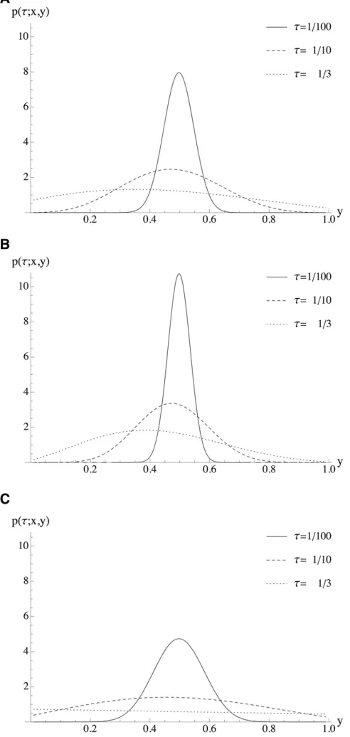
of a constant population size (cf. Figure 1A), an instanta-neous expansion (cf. Figure 1B) narrows the distribution around the mean, whereas an additional phase of a reduced population size (cf. Figure 1C) increases the variance relative to

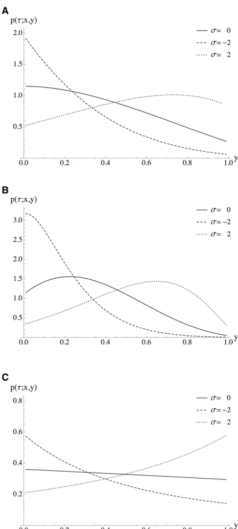
a population of a constant size. Figure 2 illustrates the same scenarios with a fixed transition time and varying selection coefficients. Note that all theoretical results and the corre-sponding applications in this article were implemented in Mathematica. The implementation is available from the authors upon request.

The Sample Frequency Spectrum

The transition density approach

The transition density derived in the previous section can be employed to obtain the SFS of a sample. Consider a sample of sizenobtained at timet¼t. The probability that theA1 allele with frequencyxat timet¼t0is observedbtimes in the sample is (Griffiths 2003)

pn;bðx;t0;tÞ ¼ Z 1

0

n b

ybð12yÞn2bpðt0;t;x;yÞdy: (13)

For piecewise-constant population size models with K epochs, a spectral representation of pðt0;t;x;yÞ can be found via (11) and evaluating (13) involves computing the integral R₀1yb_ð12yÞn2b

pK21ðyÞFK21ðyÞdy. Forl$0,

us-ing (2), (5), and (7), we obtain Z 1

0

ybð12yÞn2bpK21ðyÞFKl21ðyÞdy

¼XN

m¼0 ffiffiffiffiffiffiffiffiffiffi cK21 p

uK_l;m21 Z 1

0

yb21ð12yÞn2b21ecK21sy_G

mðyÞdy

¼XN

m¼0 ffiffiffiffiffiffiffiffiffiffi cK21 p

uK_l;m21 1 bþ1

Xm

h¼0

ð21Þhþ1

3 "

mþ1

hþ1 !

hþmþ2

h

!,

nþhþ1

bþ1 !#

31F1ðbþ1;nþhþ2;cK21sÞ;

(14)

where1F1ða;b;zÞ ¼ P

j$0aðjÞ=bðjÞzj=j!is the confluent hyper-geometric function of the first kind. The descending facto-rialsdðjÞare defined inAppendix.

The SFSqn;bðtÞis the probability distribution on the

num-berbof mutant alleles in a sample of sizentaken at timet, conditioned on segregation. For 1#b#n21, qn;bðtÞ is

given by

qn;bðtÞ ¼ lim x/0

Rt

2Npn;bðx;t0;tÞdt0 Rt

2N Pn21

a¼1pn;aðx;t0;tÞdt0

: (15)

In (15), the SFS at a single site is obtained by averaging over sample paths. This is equivalent to the frequency spectrum distribution over a large number of independent mutant sites in the Poisson randomfield model of Sawyer and Hartl

(1992). Using (11), (12), (13), and (14), we can approx-imate (15) numerically. If it is unknown which allele is derived, a folded version of (15) can be obtained as

½qn;bþqn;n2b=ð1þdb;n2bÞ, where db;n2b denotes the

Kro-necker delta.

A moment-based approach

As detailed above, the transition density can be employed to obtain the SFS. However, the specific solution for the transition density is not required to obtain the less complex and thus computationally less demanding SFS. Here, we utilize the work of Evanset al.(2007) to develop an efficient algorithm for computing the allele frequency spectrum in the case of genic selection and piecewise-constant popula-tion sizes.

Suppose mutations arise at rateu=2 (per sequence per 2Nref generations) and according to the infinitely-many-sites model (Kimura 1969). Evans et al. (2007) use the forward diffusion equation to describe population allele frequency changes and introduce mutations by an ap-propriate boundary condition. Slightly modifying their notation, we usefðy;tÞdyto denote the expected number of sites where the mutant allele has a frequency in ðy;yþdyÞ, with 0,y,1, at timet. The forward equation is

@

@tfðy;tÞ ¼ 1 2

@2

@y2fbðy;tÞfðy;tÞg2 @

@yfaðyÞfðy;tÞg; (16)

where the diffusion term bðy;tÞ ¼yð12yÞ=rðtÞ, the drift term aðyÞ ¼syð12yÞ, and the scaled selection coefficient

s and the population size functionrðtÞ are defined as be-fore. The influx of mutations is incorporated into this pro-cess via the boundary conditions

lim

yY0yfðy;tÞ ¼urðtÞ and limy[1fðy;tÞ finite: (17)

The resulting polymorphic sites follow the dynamics of (16) thereafter. Note that this differs from the diffusion process studied in the previous section, as the influx of mutations is now explicitly modeled.

Again, it is analytically more practical to consider the corresponding backward equation, which is obtained by setting gðy;tÞ:¼ yð12yÞfðy;tÞ. This substitution trans-forms the forward equation forfðy;tÞinto a backward equa-tion for gðy;tÞ, which is essentially given by (1) up to the sign of the drift term. Evanset al.(2007) derived a coupled system of ODEs for the momentsmjðtÞ ¼

RN 0 y

j_gðy;tÞdy:

m₀9ðtÞ ¼u 22

1

rðtÞm0ðtÞ þs½m0ðtÞ22m1ðtÞ; (18)

m_j9ðtÞ ¼ 1

rðtÞ "

jþ1

2 !

m_j21ðtÞ2 jþ2

2 !

m_jðtÞ #

þsðjþ1ÞmjðtÞ2ðjþ2Þmjþ1ðtÞ

; j$1; (19)

where mj9ðtÞ ¼dmjðtÞ=dt. A similar system of ODEs was

derived and solved by Kimura (1955a) for a neutral sce-nario with a constant population size and without muta-tions. For s¼0, the above system is finite and can be solved explicitly (Zivkovi´c and Stephan 2011). In the caseˇ of selection (s6¼0), on the other hand, the system is infinite and obtaining an explicit solution for an arbitrary

ris a challenging problem, even if the system is truncated by settingmjðtÞ ¼0 forj$D.

From now on, assumemjðtÞ[0 forj$Dand rewrite the

truncated system of ODEs in matrix form as

M9ðtÞ ¼ 1

rðtÞBþsA

MðtÞ þQ; (20)

where MðtÞ ¼ m½₀DðtÞ;m½₁DðtÞ;. . .;m½_DD₂₁ðtÞT, M9ðtÞ ¼ dMðtÞ=dt, Q¼ ðu=2;0;. . .;0ÞT are D-dimensional column vectors, andB¼ ðbklÞandA¼ ðaklÞareD3Dmatrices with

entries

bkl¼ 8 > > > > > < > > > > > :

2

kþ2 2

; if l¼k;

kþ1 2

; if l¼k21;

0; otherwise;

and

akl¼ 8 > < > :

kþ1; if l¼k; 2ðkþ2Þ; if l¼kþ1; 0; otherwise;

for 0#k;l#D21. The formal solution of (20) cannot be written in terms of a matrix exponential but only as a Peano–Baker series (Baake and Schlägel 2011) for arbi-trary r, which can be numerically quite demanding. There-fore, we focus on the case of piecewise constant r and develop an efficient method to solve the truncated system of ODEs.

We first consider rðtÞ[c0 (i.e., a constant population size), for which the solution of (20) takes the form of a ma-trix exponential given by

MðtÞ ¼exp

R

t 0 B c0

þsA

ds

Mð0Þ

þ (

R

_t

0exp

R

_t s B c0

þsA

du ds ) Q

¼exp B c0

þsA

t

Mð0Þ

þ (

exp B

c0 þsB

t 2I ) B

c0þsA

₂1

Q:

(21)

Let2lk;ðlk;0;. . .;lk;D21Þ, andðr0;k;. . .;rD21;kÞT, respectively,

denote the eigenvalues, row eigenvectors, and column eigenvectors ofB=c0þsA. Then, (21) implies

m½_jDðtÞ ¼X D21

i¼0

m½_iDð0ÞX D21

k¼0

rjklkie2lktþ

u

2 X D21

k¼0 rjklk0

12e2lkt lk :

(22)

It is intractable to find closed-form expressions of2lk;lki,

and rjk, but, for a given truncation level D, they can be

computed numerically. Depending on the details of the model under consideration, it might be more efficient to solve (21) numerically rather than applying the more analytic form given in (22).

We now investigate the equilibrium solution of (22), since it can be applied as an initial condition in a model in which the population size remains constant over a longer period of time before instantaneous population size changes occur. Assuming that all alleles are monomorphic at time zero, i.e., m½_iDð0Þ[0, and letting t/N, we obtain the moments at equilibrium as

b

m½_jD¼u

2 X D21

k¼0 rjklk0

lk :

ForDsufficiently large, this result is numerically close to the exact solutionbmj. The latter can also be obtained as follows.

The equilibrium population frequency spectrum is given by (Fisher 1930)

b_{fðyÞ ¼}uc0

12e22c0sð12yÞ

yð12yÞð12e22c0s_Þ: (23)

The sampled version can be easily found via binomial sampling as in (13):

b_f

n;b¼uc0 n bðn2bÞ

121F1ðb;n;2c0sÞe22c0s

12e22c0s : (24)

For s6¼0, the momentsmbjofbgðyÞ ¼yð12yÞbfðyÞ are given

by

b

m_j¼uc0 1 12e22c0s

(

e22c0s_{½Gðjþ1;22c}

0sÞ2j! ð22c0sÞjþ1

þ 1

jþ1 )

;

where Gða;zÞ ¼R_zNta21_e2t_{dt is the incomplete gamma}

function.

Now, consider the piecewise-constant model with K epochs in the time interval ½t0;t defined earlier. For

ti#t,tiþ1,

M9ðtÞ ¼ B ci

þsA

MðtÞ þQ; (25)

which can be solved as in (21). Fort.tK21,

MðtÞ ¼exp B

cK21 þsA

ðt2tK21Þ

MðtK21Þ

þ

f

exp B

cK21 þsA

ðt2tK21Þ

2I

g

B

cK21þsA

₂1

Q;

(26)

whereMðtiÞ, for 1#i#K21, is recursively given by

MðtiÞ ¼exp B ci21

þsA

ðti2ti21Þ

Mðti21Þ

þ

f

exp B ci21

þsA

ðti2ti21Þ

2I

g

B

ci21þsA

₂1

Q:

The initial condition Mðt0Þ is chosen as either the equilib-rium solution described above or the zero vector, which cor-responds to the case of all loci being monomorphic at time t0¼t0.

The accuracy of the above framework depends on how fast the truncated momentsm½_jDðtÞconverge to zero asD increases. Similar to the transition density approach, the truncated moments converge faster for negative than for positive s, and for instantaneous declines compared to instantaneous expansions. For a large positives, a higher truncation level D may be required to achieve the de-sired accuracy. Finally, the allelic spectrum fn;bðtÞ, for

1#b#n21, of a sample of size n taken at time t can

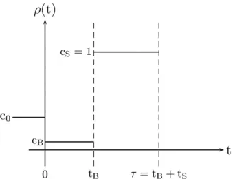
Figure 4 The population is constant in size before being instantaneously changed to relative sizecBat time zero. Then, another jump to relative population

be obtained from the moments mjðtÞ by using the

relationship

fn;bðtÞ ¼

n b

Xn2b21

l¼0 ð21Þl

n2b21 l

m_lþb21ðtÞ: (27)

The SFSqn;bðtÞat timet is then given by

qn;bðtÞ ¼

fn;bðtÞ Pn21

a¼1fn;aðtÞ

: (28)

Substituting the truncated moments obtained from (26) into (27) provides numerical approximations of (27) and (28).

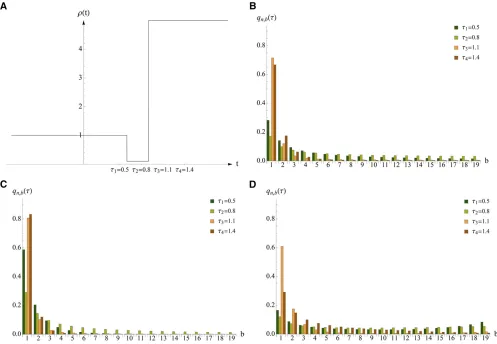
The joint impact of a population bottleneck and selection on the SFS is illustrated in Figure 3 for various points in time. As expected, negative and positive selection result in a skew of the SFS toward low- and high-frequency derived variants, respectively, when compared to a model without selection, across all sampling times. Moreover, this skew varies in intensity at different points in time. In the neutral demographic model (cf. Figure 3B), the relative frequency of singletons at timet3 is higher than at timet4, whereas under the same demographic model with negative selection (cf. Fig-ure 3C), this relation is inverted. This is because the amount of singletons that is caused by demographic forces decreases after the expansion from t3 to t4, while negative selection is still increasing the low-frequency derived classes in this time interval.

Applications

Here, we discuss biologically relevant questions that can be addressed using our theoretical framework. This section consists of the following parts:

1. Wefirst consider models with negative selection and bot-tlenecks of medium strength at different time points. We examine the SFS under such models and try to estimate the demographic parameters while taking selection into account. We also carry out demographic inference ignor-ing selection. Whereas the former demonstrates how well the demographic and selective parameters can be esti-mated jointly, the latter mimics the common practice of assuming genome-wide polymorphic sites as putatively neutral (due to the difficulty of jointly estimating the impact of selection and demography using existing tools). Wefinally examine the consequences of assuming

a too simple underlying demography on parameter estimation.

2. We then analyze an African sample ofD. melanogasterto investigate its demographic history and possible selective effects.

3. Finally, we examine a model of strong exponential pop-ulation growth (mimicking human evolution) and su-perimpose negative selection of various strengths to understand if and when selection can be inferred for such a model.

Throughout, the first population size change will occur after the allele frequencies have reached an equilibrium according to (24).

Joint inference of population bottleneck and purifying selection

A maximum likelihood approach: Under the assumption

that the considered sites are independent, the log-likelihood of a model Mgiven data Dis log½LðD;MÞ ¼ Pn21

i¼1dilogðqiÞ þconstant, wheredi is the observed number

of sites at which the derived allele occurs i times in the sample, and qi is the probability that the derived allele

occurs i times in the sample at a segregating site under model M (e.g., Wooding and Rogers 2002). Recall thatqi

can be obtained via either the transition density or the moment-based approach. The latter is preferable here, since the transition density is not explicitly required.

Consider the bottleneck model illustrated in Figure 4. Note that the present relative sizecS isfixed to 1;i.e., here the present population size is used as the reference popula-tion size Nref. First, we consider the scenario where the ancestral population size c0 prior to the bottleneck is allowed to vary. In this case, the model hasfive free param-eters:c0, the initial population size;cB, the population size during the bottleneck; tB, the duration of the bottleneck; tS¼t2tB, the time since recovery from the bottleneck; ands, the scaled selection coefficient. We then also consider

the scenario where the ancestral population size is the same as the present population size, i.e., c0¼cS, resulting in a model with four free parameters.

We adopted a grid search in our estimation procedure, with s2 ½210;0 and cB;tB;tS2 ½0:001;1. For the five-parameter model, c0 was chosen from the range½0:01;10. In total, 110,000 grid points were chosen in the selected case and 10,000 in the neutral case. Note that the grid search also accounts for models of one or two successive

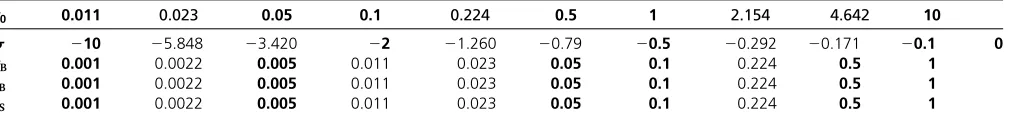
Table 1 Grid values chosen for each parameter in our optimization procedure

c0 0.011 0.023 0.05 0.1 0.224 0.5 1 2.154 4.642 10

s 210 25.848 23.420 22 21.260 20.79 20.5 20.292 20.171 20.1 0

cB 0.001 0.0022 0.005 0.011 0.023 0.05 0.1 0.224 0.5 1

t_B 0.001 0.0022 0.005 0.011 0.023 0.05 0.1 0.224 0.5 1

t_S 0.001 0.0022 0.005 0.011 0.023 0.05 0.1 0.224 0.5 1

The underlying bottleneck model is illustrated in Figure 4. Grid valuesc0were considered for thefive-parameter model, whereasc0¼cSin the four-parameter model. The

instantaneous population expansions. For the four-parameter model, 11,000 grid points were chosen in the selected case and 1000 in the neutral case. The grid points are summarized in Table 1.

Estimation of bottleneck and selection parameters: We

first evaluated the SFS for a sample of size n¼50 in the following 12 scenarios, all with cS ¼1 and

s2 f0;21=2;22g:

1. constant population size (i.e.,c0¼cB¼cS¼1).

2. bottleneck models with c0¼1=2;cB¼1=10, tB¼1=10, andtS2 f1=200; 1=20; 1=2g.

First, to test how well the demographic and selective parameters can be estimated jointly from sampled data, we focused on the bottleneck demography withtS ¼1=20 and considered two scenarios: The neutral case (s¼0) and the selected case withs¼ 22. To mimic the limited availabil-ity of independent polymorphic sites across the genome, we sampled 10,000 sites according to the SFS for the two chosen scenarios and repeated this procedure 200 times. For each of these 200 data sets, we maximized the log-likelihood over the grid of parameter values described earlier, assuming (A1) neutrality when the true model hass¼0, (A2) neutrality when the true model hass¼ 22, (A3) presence of selection when the true model has s¼ 22, and (A4) pres-ence of selection when the true model hass¼0.

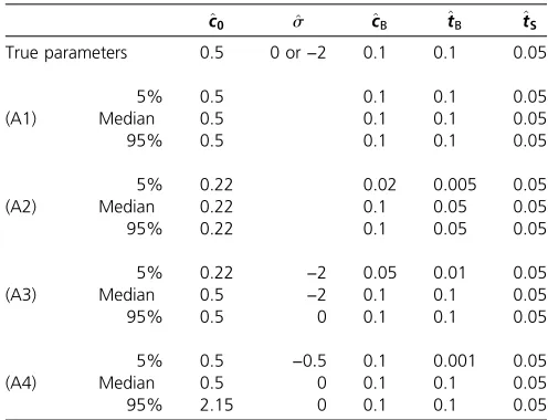
The estimated parameters are shown in Table 2. For in-ference under correct model assumptions (A1 and A3), the median estimates are equal to the true parameters. When selection is ignored although present in the data set (A2), the ancestral population size (c0) and the duration of the

bottleneck (tB) are underestimated, whereas the bottleneck size (cB) and the time since the bottleneck (tS) are accurately estimated. When the true model is neutral but the inference procedure allows for selection (A4), a neutral demographic model is accurately inferred. We calculated likelihood-ratio statistics for each of the 200 data sets to compare the two nested models of selection and neutrality. The null hypothesis of neutrality can be rejected at the 5% significance level with a power of 55%.

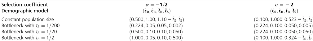
We further analyzed all 12 scenarios using the expected SFS directly, assuming that the amount of data are suffi-ciently large such that the observed SFS closely approx-imates the expected value. Our goal in this case is to study the effect of model misspecification on parameter estima-tion; specifically, assuming selection when the true model is neutral or assuming neutrality when there is selection. In the former case, the maximum likelihood estimates (MLEs) always coincided with the true parameters. Therefore, it is useful to allow for selection in an analysis even when putatively neutral regions are considered. In the latter case, our results are summarized in Table 3. For a constant pop-ulation size, two rather old instantaneous expansions are estimated. For the bottleneck models, ignoring selection leads to the largest errors for the most recent bottleneck and

s¼21=2 and the least recent bottleneck and s¼ 22, for which an instantaneous expansion is estimated. The time since the bottleneck was robustly estimated in many cases.

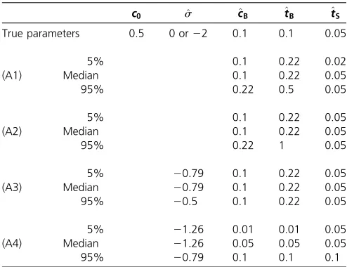
To assess the impact of assuming a slightly simplified model for parameter estimation, we carried out an analo-gous study in which the ancestral population size c0 was incorrectly assumed to equal the current size cS¼1, while the true model hadc0¼1=2 andcS¼1. For the resampling analysis, we considered the same bottleneck scenarios as before withs¼0 or22, and maximized the log-likelihood values over a grid in the parameter space (as described earlier) for each of the 200 simulated data sets each con-taining 10,000 polymorphic sites. The parameter estimates are shown in Table 4. The time since the bottleneck (tS) is accurately estimated irrespective of correct or wrong assump-tions regarding selection. Incorrectly assumingc0¼cSresults in either an overestimation of the duration of the bottleneck (tB) in most of the cases (A1–A3) or an inference of selec-tion whens¼0 (A4). Selection was poorly estimated even under (A3).

Again, we also analyzed all 12 scenarios under the assumption that the observed SFS is a close approximation to the expected value, to study the effect of model misspecification on parameter estimation. The results are shown in Table 5. The biases caused by incorrectly assuming c0¼cS are largest for the scenario that captures the

youn-gest bottleneck (tS¼1=200). Here, not only the selection

coefficients are strongly misestimated but also the time since the bottleneck (tS) is largely underestimated. In all the other

scenarios, at least the time since the bottleneck (tS) is

accu-rately estimated. The estimation accuracy of the other de-mographic parameters and selection coefficients increases

Table 2 Parameter estimation results based on 10,000 sampled sites

^

c0 ^s ^cB ^tB ^tS

True parameters 0.5 0 or−2 0.1 0.1 0.05

5% 0.5 0.1 0.1 0.05

(A1) Median 0.5 0.1 0.1 0.05

95% 0.5 0.1 0.1 0.05

5% 0.22 0.02 0.005 0.05

(A2) Median 0.22 0.1 0.05 0.05

95% 0.22 0.1 0.05 0.05

5% 0.22 −2 0.05 0.01 0.05

(A3) Median 0.5 −2 0.1 0.1 0.05

95% 0.5 0 0.1 0.1 0.05

5% 0.5 −0:5 0.1 0.001 0.05

(A4) Median 0.5 0 0.1 0.1 0.05

95% 2.15 0 0.1 0.1 0.05

SFS were computed for the true parameters and the demography illustrated in Figure 4 (c0¼1=2,cS¼1). Then, 10,000 sites were sampled according to the SFS of the neutral

with bottleneck age and the concomitant decreasing impact of the ancestral population size on the SFS. In summary, we note that assuming a too simplistic demographic model can lead to large errors in parameter estimation.

Testing a data set of D. melanogaster:Here, we apply our

method to analyze a data set that has been recently used to estimate the joint demographic history of several popula-tions ofD. melanogaster(Duchenet al., 2013). The data set consists of 12 sequences from a Zimbabwe population com-prising 197 noncoding loci, and within each locus there are between 1 and 41 segregating sites (3234 polymorphic sites in total). We focused on the effects of weak selection and used all segregating sites in our analysis, treating them as independent. We note that whereas the 197 loci are scat-tered over the genome, at least tens of thousands of bases apart, the sites within each locus are tightly linked and hence not independent. We have tried a bootstrap resampling procedure to study the effect of assuming independence, but the strong stochasticity among the small subsets of presumably independent sites, which were generated by sampling one site from each locus, prevented a reliable inference.

The empirical SFS of the data shows an uptick of high-frequency derived alleles (cf. Figure 5A). As explained in Discussion, this is likely to be caused by ancestral misidenti-fication, not by positive selection. This effect is also unlikely to be caused by linkage, since the uptick is still observed in the previously mentioned subsamples of widely separated sites. To assess the effect of presumably misoriented sites on inference, we compare results for the unfolded SFS with those obtained from a partly folded version, where only singletons and doubletons are folded with their high-frequency counterparts, since these classes appear to be affected the most (cf. Baudry and Depaulis 2003).

We carried out our analysis based on the bottleneck model of the previous section allowing the current and the ancestral population size to differ. To account for varying selection pressures across the genome, sites are usually subdivided into various genomic categories (e.g., exons, introns, UTRs), often assuming a constant selection coeffi-cient for each category. Alternatively, or even combined with such a categorization, selection coefficients are assumed to follow some distribution; a gamma distribution (Kimura 1979) is a popular choice due to itsflexibility tofit empirical

data. Since neutrality and purifying selection are considered to be prevalent in intronic and intergenic regions of African Drosophila, we focused on negative selection coefficients in our analysis. A noncoding data set can be classified as a sin-gle functional category. Therefore, we analyzed the data set first by either assuming constant selection or neutrality, fol-lowed by an analysis where the selection coefficients were allowed to vary according to a given distribution.

We initially computed an MLE for the unfolded and the partly folded SFS under the constant selection and the neutral bottleneck model on the coarse parameter grid given in Table 1. For each model, we investigated the accuracy of the parameter estimates via parametric bootstrap, using 200 bootstrap samples each consisting of 3234 polymorphic sites. We obtained rather narrow confidence intervals for the selection coefficient and the time since the bottleneck, whereas the other details of the bottleneck were less confi-dently estimated. To improve the parameter estimates, we further refined the grid as follows: Nine values forc0 were chosen from the range½0:5;10, 20 values forsfrom½22;0, 10 values forcB from½0:001;0:1, 25 values fortB=cB from ½0:84;3:31, and 25 values fortSfrom½0:05;0:22. This gives in total 1,125,000 parameter combinations for selection and 56,250 for neutrality. As before, the ratio of two consecutive values in each parameter range was kept roughly constant. Focusing on rescaled time tB=cB instead of tB relies on the observation thattB andcB correlate strongly and has the ad-vantage that unlikely combinations oftBandcBcan be omitted.

More values were chosen for time parameters, since these are more sensitive than the population size parameters.

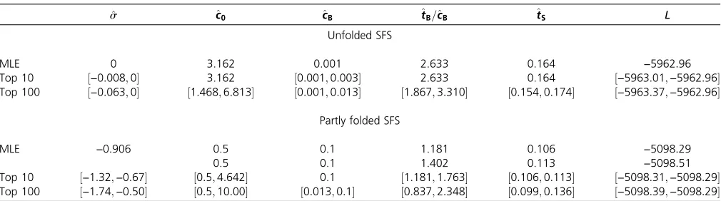
The MLEs are given in Table 6 and both versions of the SFS are illustrated in Figure 5. The analysis based on the partly folded SFS shows a betterfit than the unfolded version, since negative selection combined with any demographic model is incompatible with the uptick of high-frequency de-rived variants in the empirical SFS. Interestingly, a neutral model was inferred for the unfolded SFS, while the model with selection fits better for the partly folded version. Since an ex-cess of high-frequency derived variants favors demographic models that capture a strong population decline, a much smaller estimate of the bottleneck population size (cB) was obtained for the unfolded SFS. In accordance with the previous section, the time since the bottleneck (tS) was robustly estimated in both cases, as illustrated by the 10 and 100 most

Table 3 Parameter estimation results based on the expected SFS assuming neutrality when the true model is under selection

Selection coefficient s¼21=2 s¼ 22

Demographic model ð^c0;^cB;^tB;^tSÞ ð^c0;^cB;^tB;^tSÞ Constant population size ð0:500;1:00;1:102^tS;^tSÞ ð0:100;1:000;0:5232^tS;^tSÞ Bottleneck withtS¼1=200 ð0:224;0:05;0:05;0:002Þ ð0:224;0:100;0:050;0:005Þ

Bottleneck withtS¼1=20 ð0:500;0:10;0:10;0:050Þ ð0:224;0:100;0:050;0:050Þ

Bottleneck withtS¼1=2 ð1:000;0:05;0:10;0:500Þ ð0:100;1:000;0:3242^tS;^tSÞ

SFS were computed for the following demographic scenarios and selection coefficients. In terms of the demography, either a constant population size or a bottleneck model according to Figure 4 with parametersc0¼1=2,cB¼1=10,cS¼1,tB¼1=10 andtS¼1=200, 1=20 or 1=2 was assumed. The selection coefficients ares¼21=2 and22.

likely parameter estimates. However, partially folding the SFS led to a smaller estimatebtS. A further refinement of the grid barely changed the estimatesbtS andbcB. The estimates of bottleneck duration (tB) and ancestral population size (c0) appeared to be strongly correlated.

We now relax the assumption of a fixed s for all sites and allow a distribution of fitness effects by introducing gamma-distributed selection coefficients. Fors.0, the proba-bility density of the gamma distribution with shape and rate parametersaand bis given bygðsÞ ¼ bðbsÞa21e2bs_=GðaÞ,

where GðÞdenotes the gamma function. The allelic spectrum for gamma-distributed selection coefficients is then obtained by integrating the allelic spectrum for constant selection coefficients given by (27) against a gamma distribution,i.e.,

~ fn;bðtÞ ¼

Z 0

2Nfn;bðt;sÞgð2sÞds: (29) The SFS for gamma-distributed selection coefficients is then given by

~ qn;bðtÞ ¼

~ fn;bðtÞ Pn21

a¼1~fn;aðtÞ

:

Even when the allelic spectrum is in equilibrium and the population size is constant, the integral in (29) cannot be solved explicitly, so we needed to employ numerical in-tegration. Previous studies (e.g., Boyko et al.2008; Racimo and Schraiber 2014) on the distribution offitness effects in the presence of population size changesfirst inferred a de-mographic history using putatively neutral sites and then estimated the parametersaandbbased on thatfixed demog-raphy. Since we do not have a separately inferred demographic model here, we considered severalsvalues along a variety of demographic parameter combinations. We used a coarser grid for the demographic parameters due to the larger number ofs

values needed for the numerical integration step, which adds additional computational burden. While the evaluation of the allelic spectrum takes less than half a second for a givensvalue with high numerical precision, the numerical integration over the range ofs values according to (29) takes a few seconds. Thus, to further reduce computational cost, we restricted the analysis to exponentially distributed selection coefficients by set-tinga¼1 and compared the MLEs for various values ofb. See Table 7 for results. The MLE was found forb¼1, so the average

sequals2a=b¼ 21. Thisfinding and the associated demo-graphic estimates are consistent with the result found for afixed selection coefficient. However, this result may change if one allows for more general shape and rate parameters.

A model of human exponential population growth

We now demonstrate the utility of our method to investigate population-size histories containing epochs of exponential growth in combination with selection. To this end, we

Table 4 Parameter estimation results based on 10,000 sampled sites when the ancestral population sizec0is incorrectly assumed to equal the current sizecS, while the true model hasc0¼1=2andcS¼1

c0 ^s ^cB ^tB ^tS

True parameters 0.5 0 or22 0.1 0.1 0.05

5% 0.1 0.22 0.02

(A1) Median 0.1 0.22 0.05

95% 0.22 0.5 0.05

5% 0.1 0.22 0.05

(A2) Median 0.1 0.22 0.05

95% 0.22 1 0.05

5% 20:79 0.1 0.22 0.05

(A3) Median 20:79 0.1 0.22 0.05

95% 20:5 0.1 0.22 0.05

5% 21:26 0.01 0.01 0.05

(A4) Median 21:26 0.05 0.05 0.05

95% 20:79 0.1 0.1 0.1

SFS were computed for the true parameters and the demography illustrated in Figure 4 (c0¼1=2,cS¼1). Then, 10,000 sites were sampled according to the SFS of the neutral

and the selective scenario, and this procedure was repeated 200 times each. The log-likelihood values were maximized over the four-parameter space (wherec0¼cSis

as-sumed), and the table reports the median, the 0.05 and the 0.95 quantiles. The four cases correspond to assuming (A1) neutrality whens¼0, (A2) neutrality whens¼22, (A3) presence of selection whens¼22, and (A4) presence of selection whens¼0.

Table 5 Parameter estimation results based on the expected SFS when the ancestral population sizec0is incorrectly assumed to equal the current sizecS, while the true model hasc0¼1=2andcS¼1

Selection coefficient s¼0 s¼21=2 s¼ 22

Demographic model ðs^;^cB;^tB;^tSÞ ðs^;^cB;^tB;^tSÞ ð^s;^cB;^tB;^tSÞ

ð^cB;^tB;^tSÞ ð^cB;^tB;^tSÞ ð^cB;^tB;^tSÞ Bottleneck withtS¼1=200 ð23:420;0:023;0:050;0:001Þ ð20:171;0:224;0:224;0:011Þ ð25:848;0:023;0:050;0:001Þ

ð0:224;0:224;0:011Þ ð0:224;0:224;0:011Þ ð0:023;0:100;0:001Þ

Bottleneck withtS¼1=20 ð21:260;0:050;0:050;0:050Þ ð22:;0:050;0:050;0:050Þ ð20:794;0:100;0:224;0:050Þ

ð0:100;0:224;0:050Þ ð0:100;0:224;0:050Þ ð0:100;0:224;0:050Þ

Bottleneck withtS¼1=2 ð20:292;0:224;0:500;0:500Þ ð0;0:050;0:100;0:500Þ ð22:;0:224;0:500;0:500Þ

ð0:224;0:500;0:500Þ ð0:050;0:100;0:500Þ ð0:050;0:224;0:500Þ SFS were computed for the following demographic scenarios and selection coefficients. In terms of the demography, a bottleneck model was assumed according to Figure 4 with parametersc0¼1=2,cB¼1=10;tB¼1=10 andtS¼1=200, 1=20, or 1=2. The selection coefficients were chosen ass¼0,21=2, and22. The parameter estimates

were obtained according to the model assumingc0¼cS(the grid for the four-parameter space being a subset of the grid for thefive-parameter space) and by assuming

adopted the following demographic history of a sample of African human exomes that had been estimated by Tennessen et al. (2012) as a modification of a model by Gravel et al. (2011). The population had an ancestral size of 7310 individ-uals until 5920 generations ago (assuming a generation time of 25 years), when it increased instantaneously in size to 14,474 individuals. After this increase, the population remained con-stant in size until 205 generations ago, when it started to grow exponentially until reaching 424,000 individuals at present. The relative population size function for this model can be described by

rðtÞ ¼ 8 < :

1; t,0;

c; 0#t,te;

cexp½Rðt2teÞ; te#t#t;

(30)

wherecis the ratio of population sizes after and before the instantaneous expansion, which can be dated arbitrarily, so we set the time of this expansion to zero. R is the scaled exponential growth rate,teis the time at which the expan-sion started, and t is the time of sampling (the present). Times are given in units of 2Nref, where the reference population

size Nref is the initial size before time zero (the ancestral size). Since the theoretical framework presented above assumes a history of piecewise constant population sizes, the phase of exponential growth in this model had to be adequately discretized to obtain a suitable piecewise approx-imation. The following piecewise function can be chosen to approximate the exponential growth phase via a geometric growth function,

qðtÞ ¼ 8 < :

1; t,0;

c; 0#t,t1; cð1þdÞi; ti#t,tiþ1;

(31)

with timesti¼teþlog½ð1þdÞi21ð2þdÞ=2=R,i¼1;. . .;it.

Here, the number of population size changes during the phase of exponential growth is given by

it:¼

⌊

Rðt2teÞ2logðd=2þ1Þ logðdþ1Þ

⌋

þ1:

Varying the growth rateddetermines the number of discre-tization intervals used.

Figure 5 (A) SFS for the observed data and the most likely selective and neutral parameter estimates from left to right. (B) The same as A except that the allelic classes 1 and 2 were respectively folded with 11 and 10.

Table 6 Parameter estimation results based on the unfolded and the partly folded SFS and constant selection coefficients

^

s ^c0 ^cB ^tB=^cB ^tS L

Unfolded SFS

MLE 0 3.162 0.001 2.633 0.164 −5962:96

Top 10 ½−0:008;0 3.162 ½0:001;0:003 2.633 0.164 ½−5963:01;−5962:96

Top 100 ½−0:063;0 ½1:468;6:813 ½0:001;0:013 ½1:867;3:310 ½0:154;0:174 ½−5963:37;−5962:96

Partly folded SFS

MLE −0:906 0.5 0.1 1.181 0.106 −5098:29

0.5 0.1 1.402 0.113 −5098:51

Top 10 ½−1:32;−0:67 ½0:5;4:642 0.1 ½1:181;1:763 ½0:106;0:113 ½−5098:31;−5098:29

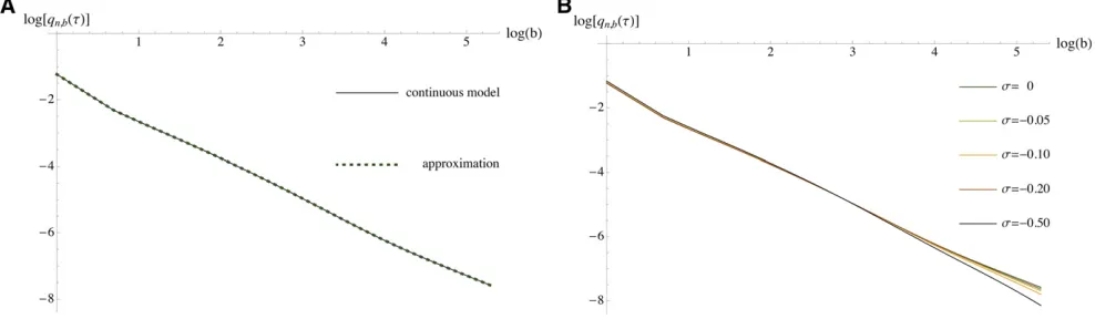
The SFS (28) of the discretized version is obtained straightforwardly from (26) and (27). For the demographic parameters given above, we computed the SFS for various sample sizes up to 200 and we used d¼1=4, which was chosen large enough to provide reasonably fast computation times but sufficiently small to provide a good approximation of the exponential growth model. In the neutral case, the goodness of the approximation can be verified via the ex-plicit solution of the SFS (Zivkovi´c and Stephan 2011),ˇ which can be applied to the continuous and the discretized model. As shown in Figure 6A, where a sample size of n¼200 is chosen, the spectra of both continuous and piece-wise-constant models agree very well with each other; the percentage error is 0.57% based on thel2_{-norm, while the} Kullback–Leibler divergence is about 1:7631027_.

Using our method, selection can then be incorporated into the piecewise-constant population-size model. The effect of various negative selection coefficients (scaled with respect to the ancestral population size) is illustrated again

for sample size n¼200 in Figure 6B, and the same trend can be observed for smaller sample sizes as well. It is prob-ably not surprising that the resolution in distinguishing the selective and the neutral model rises with s. More interest-ingly, differences between the neutral and the selective models are apparently more pronounced among derived alleles in in-termediate to high frequency. Therefore, for large data sets where intermediate- to high-frequency derived alleles are pres-ent in sufficipres-ent numbers, one may focus more strongly on these allelic classes than on low-frequency derived ones for the statistical analysis of purifying selection.

Discussion

In this article, we extended the approach of Song and Steinrücken (2012) to develop a method forfinding the transition density of a WF diffusion under genic selection and piecewise-constant effective population sizes. It can be used to obtain the SFS, but explicit knowledge of the transition density is actually not re-quired for the computation of the SFS. To that end, we revis-ited and simplified the moment-based method by Evanset al. (2007) in the case of a constant population size and utilized the result to obtain an efficient method for computing the SFS for a model with piecewise-constant population sizes.

The transition density for a variable population size can be incorporated into a hidden Markov model framework to analyze time series genetic data, as done by Steinrücken et al.(2014) in the case of a constant population size. How-ever, in this article we focused on biological questions that can be investigated using the SFS and sampling at a single time point. The SFS has been employed into a maximum likelihood framework that can be applied tosimultaneously infer selection coefficients and the parameters of a multi-epoch demographic model. The importance of methods that enable the joint estimation of selective and demographic parameters becomes particularly apparent in large populations, for which the scaled selection coefficient can take considerable values across large regions of the genome, so that demog-raphy and selection cannot be estimated independently.

Table 7 Parameter estimation results for partly folded SFS and exponentially distributed selection coefficients

b ^c0 ^cB ^tB=^cB ^tS L

0.1 2 0.01 0.631 0.126 25101.36

0.2 2 0.05 1 0.158 25098.59

0.5 1 0.1 1.584 0.1 25098.50

1 0.5 0.1 1.259 0.1 25098.43

2 2 0.1 2.508 0.126 25098.69

5 0.5 0.1 1.259 0.126 25098.67

10 0.5 0.1 1.259 0.126 25098.73

20 0.5 0.1 1.259 0.126 25098.79

50 0.5 0.1 1.259 0.126 25098.84

100 0.5 0.1 1.259 0.126 25098.86

The demographic histories were estimated based on exponentially distributed selection coefficients and for the demographic model illustrated in Figure 4 for the entire data set of 3234 polymorphic sites. First, allelic spectra were evaluated for 12,600 different demographic parameter combinations and 100svalues each. Then, polynomial curves of degree 3 werefitted between successivesvalues and for every single demographic parameter combination, before a numerical integration against a gamma distribution witha¼1 and 10 different values ofbwas applied. From the allelic spectra, now being corrected for varying selection coefficients, the SFS were obtained. The resultant MLEs are shown for the various choices ofb.

We tested our inference method on simulated data, generated by sampling a large number of sites from the SFS of a bottleneck model for a range of selection strengths. In our parameter estimation procedure, we assumed the same model as the one used in simulations, as well as a slightly less complex model. We demonstrated that our method can accurately estimate the parameters in the majority of the bottleneck scenarios, but less so when the simpler model is assumed. The time since the bottleneck was retrieved in most of the cases even when assuming the simpler model or when the data sets simulated with selection were analyzed under neutrality. This result is encouraging for the many published demographic esti-mates that have been obtained assuming neutrality, but further investigation is warranted to consider more realistic models,e.g., including phases of exponential growth. Our results encourage the application of not too simple demo-graphic models anyway.

In the AfricanDrosophilasample, no or barely any nega-tive selection was inferred when the possible impact of misoriented sites was ignored. To account for ancestral mis-identification while maintaining sufficient information for inference, we applied a partly folded spectrum, where only thefirst two classes were folded with the corresponding last two classes. Using this partly folded spectrum, a negative selection coefficient of abouts¼ 21 was estimated, irre-spective of assuming constant or exponentially distributed selection coefficients.

Our analyses were performed based on the bottleneck model illustrated in Figure 4. The maximum number of piecewise changes that can be incorporated into a demo-graphic model is a function of sample size (cf. Bhaskar and Song 2014 for the neutral case), so more elaborate demo-graphic models would have been barely accessible for this data set, especially given the limited amount of segregating sites. It indeed turned out to be difficult to pinpoint the ancestral population size and the duration of the bottleneck, whereas the time since the bottleneck was again robustly estimated. Comparing both versions of the SFS obtained using our parameter estimates and the ones given in Duchen et al. (2013), we obtained an improved goodness-of-fit to the observed SFS from the data and date the bottleneck as about half as old (in rescaled, but also in calendar time) based on the partly folded SFS. This discrepancy is not sur-prising, since primarily summary statistics of the SFS were used in their study while accounting for linkage to some extent.

We also applied a grid search to test if weak positive selection could explain the uptick of high-frequency derived variants in the unfolded empirical SFS. However, we did not obtain estimates being plausible from a biological point of view. When, as in this example, an excess of low- and high-frequency derived variants is simultaneously observed in comparison to a standard neutral model, unrealistically large estimates forsare needed to explain the data. Positive selection on its own (and of some appreciable strength)

causes a decline of low-frequency derived variants and an excess of high-frequency derived alleles, whereas an expan-sion (as embedded in the bottleneck model) acts in the opposite way. Therefore, both forces have to severely coun-teract each other so that the requirements of both ends of the SFS can be met.

We analyzed an example of exponential human popula-tion growth (Tennessen et al. 2012) to see the effect of purifying selection in the context of this model. As illus-trated in Figure 6B for a sample of size 200 and various selection coefficients, intermediate- and high-frequency de-rived variants are more affected by exponential growth and negative selection than the low-frequency derived ones. A plausible explanation is that both exponential growth and negative selection enforce an increase of low-frequency de-rived variants until these classes are saturated and their impact can be observed in the complimentary high-frequency allelic classes. In general, this example illustrates nicely that even more elaborate models that include various phases of exponential growth and population declines can be computa-tionally efficiently treated via an appropriate discretization of phases of continuous population size change, using the meth-ods presented in this article.

Acknowledgments

We thank valuable comments and suggestions from two reviewers. D.Z. thanks Anand Bhaskar, Steven N. Evans, and Andreas Wollstein for helpful discussions. We thank the generous support of the Simons Institute for the Theory of Computing, where much of this work was carried out while we were participating in the 2014 program on“Evolutionary Biology and the Theory of Computing.”Y.S.S. thanks the Miller Institute for providing a Research Professorship while this article was completed. This research is supported in part by Deutsche Forschungsgemeinschaft grant STE 325/14 from the Priority Program 1590 (D.Z., W.S.), the Volkswagen Foundation grant I/84232 (D.Z.), a National Institutes of Health grant R01-GM094402 (M.S., Y.S.S.), and a Packard Fellowship for Science and Engineering (Y.S.S.).

Literature Cited

Baake, M., and U. Schlägel, 2011 The Peano–Baker series. Proc. Steklov Inst. Math. 275: 155–159.

Barbour, A., S. Ethier, and R. Griffiths, 2000 A transition function expansion for a diffusion model with selection. Ann. Appl. Probab. 10: 123–162.

Baudry, E., and F. Depaulis, 2003 Effect of misoriented sites on neutrality tests with outgroup. Genetics 165: 1619–1622. Bhaskar, A., and Y. S. Song, 2014 Descartes’rule of signs and the

identifiability of population demographic models from genomic variation data. Ann. Stat. 42: 2469–2493.

Duchen, P., D. Zivkovi´c, S. Hutter, W. Stephan, and S. Laurent,ˇ 2013 Demographic inference reveals African and European admixture in the North AmericanDrosophila melanogaster pop-ulation. Genetics 191: 291–301.

Evans, S. N., Y. Shvets, and M. Slatkin, 2007 Non-equilibrium theory of the allele frequency spectrum. Theor. Popul. Biol. 71: 109–119.

Fisher, R. A., 1930 The Genetical Theory of Natural Selection. Clarendon Press, Oxford.

Fu, Y.-X., 1995 Statistical properties of segregating sites. Theor. Popul. Biol. 48: 172_–197.

Glinka, S., L. Ometto, S. Mousset, W. Stephan, and D. De Lorenzo, 2003 Demography and natural selection have shaped genetic variation in Drosophila melanogaster: a multi-locus approach. Genetics 165: 1269–1278.

Gravel, S., B. M. Henn, R. N. Gutenkunst, A. R. Indap, G. T. Marth

et al., 2011 Demographic history and rare allele sharing among human populations. Proc. Natl. Acad. Sci. USA 108: 11983–11988.

Griffiths, R. C., 2003 The frequency spectrum of a mutation, and its age, in a general diffusion model. Theor. Popul. Biol. 64: 241–251.

Griffiths, R. C., and S. Tavaré, 1994 Sampling theory for neutral alleles in a varying environment. Philos. Trans. R. Soc. Lond. B Biol. Sci. 344: 403–410.

Griffiths, R. C., and S. Tavaré, 1998 The age of a mutation in a general coalescent tree. Stochast. Models 14: 273–295. Gutenkunst, R. N., R. D. Hernandez, S. H. Williamson, and C. D.

Bustamante, 2009 Inferring the joint demographic history of multiple populations from multidimensional SNP frequency data. PLoS Genet. 5: e1000695.

Kaj, I., and S. M. Krone, 2003 The coalescent process in a popula-tion of stochastically varying size. J. Appl. Probab. 40: 33–48. Karlin, S., and H. Taylor, 1981 A Second Course in Stochastic Processes.

Academic Press, San Diego.

Kimura, M., 1955a Solution of a process of random genetic drift with a continuous model. Proc. Natl. Acad. Sci. USA 41: 144–150. Kimura, M., 1955b Random genetic drift in multi-allelic locus.

Evolution 9: 419–435.

Kimura, M., 1955c Stochastic processes and distribution of gene frequencies under natural selection, pp. 33–53 inCold Spring Harbor Symposia on Quantitative Biology, Vol. 20. Cold Spring Harbor Laboratory Press, Cold Spring Harbor, NY.

Kimura, M., 1969 The number of heterozygous nucleotide sites maintained in afinite population due to steady flux of muta-tions. Genetics 61: 893–903.

Kimura, M., 1979 Model of effectively neutral mutations in which selective constraint is incorporated. Proc. Natl. Acad. Sci. USA 76: 3440_–3444.

Krone, S. M., and C. Neuhauser, 1997 Ancestral processes with selection. Theor. Popul. Biol. 51: 210_–237.

Lenski, R. E., 2011 Evolution in action: a 50,000-generation sa-lute to Charles Darwin. Microbe 6: 30–33.

Luki´c, S., and J. Hey, 2012 Demographic inference using spectral methods on SNP data, with an analysis of the human out-of-Africa expansion. Genetics 192: 619–639.

Nei, M., T. Maruyama, and R. Chakraborty, 1975 The bottleneck effect and genetic variabiliy in populations. Evolution 29: 1–10. Racimo, F., and J. G. Schraiber, 2014 Approximation to the dis-tribution offitness effects across functional categories in human segregating polymorphisms. PLoS Genet. 10: e1004697. Sawyer, S. A., and D. L. Hartl, 1992 Population genetics of

poly-morphism and divergence. Genetics 132: 1161–1176.

Slatkin, M., and R. R. Hudson, 1991 Pairwise comparisons of mitochondrial DNA sequences in stable and exponentially grow-ing populations. Genetics 129: 555–562.

Song, Y. S., and M. Steinrücken, 2012 A simple method forfi nd-ing explicit analytic transition densities of diffusion processes with general diploid selection. Genetics 190: 1117–1129. Steinrücken, M., A. Bhaskar, and Y. S. Song, 2014 A novel spectral

method for inferring general diploid selection from time series genetic data. Ann. Appl. Stat. 8: 2203–2222.

Steinrücken, M., Y. Wang, and Y. S. Song, 2013 An explicit transition density expansion for a multi-allelic Wright_–Fisher diffusion with general diploid selection. Theor. Popul. Biol. 83: 1_–14.

Stephan, W., and H. Li, 2007 The recent demographic and adap-tive history ofDrosophila melanogaster. Heredity 98: 65_–68. Tennessen, J. A., A. W. Bigham, T. D. O_’Connor, W. Fu, E. Eimear

et al., 2012 Evolution and functional impact of rare coding variation from deep sequencing of human exomes. Science 337: 64_–69.

Watterson, G. A., 1984 Allele frequencies after a bottleneck. Theor. Popul. Biol. 26: 387_–407.

Williamson, S. H., R. Hernandez, A. Fledel-Alon, L. Zhu, R. Nielsen

et al., 2005 Simultaneous inference of selection and popula-tion growth from patterns of variapopula-tion in the human genome. Proc. Natl. Acad. Sci. USA 102: 7882–7887.

Wooding, S., and A. Rogers, 2002 The matrix coalescent and an application to human single-nucleotide polymorphisms. Genet-ics 161: 1641–1650.

Zhao, L., X. Yue, and D. Waxman, 2013 Complete numerical so-lution of the diffusion equation of random genetic drift. Genetics 194: 973–985.

ˇ

Zivkovi´c, D., and W. Stephan, 2011 Analytical results on the neu-tral non-equilibrium allele frequency spectrum based on diffu-sion theory. Theor. Popul. Biol. 79: 184–191.

ˇ

Zivkovi´c, D., and T. Wiehe, 2008 Second-order moments of seg-regating sites under variable population size. Genetics 180: 341–357.