Nonparametric Spatial analysis in spectral and space domains

(1)

KIM, HYON-JUNG. Variance Estimation in Spatial Regression Using a

Nonpara-metric Semivariogram Based on Residuals. (Under the direction of Professor Dennis

D. Boos.)

The empirical semivariogram of residuals from a regression model with stationary

errors may be used to estimate the covariance structure of the underlying process.

For prediction (Kriging) the bias of the semivariogram estimate induced by using

residuals instead of errors has only a minor effect because the bias is small for small

lags. However, for estimating the variance of estimated regression coefficients and

of predictions, the bias due to using residuals can be quite substantial. Thus we

propose a method for reducing the bias in empirical semivariogram estimates based

on residuals. The adjusted empirical semivariogram is then isotonized and made

positive definite and used to estimate the variance of estimated regression coefficients

in a general estimating equations setup. Simulation results for least squares and

robust regression show that the proposed method works well in linear models with

(2)

2

Spectral Analysis with Spatial Periodogram and Data Tapers. (Under the

direc-tion of Professor Montserrat Fuentes.)

The spatial periodogram is a nonparametric estimate of the spectral density, which

is the Fourier Transform of the covariance function. The periodogram is a useful tool

to explain the dependence structure of a spatial process. Tapering (data filtering)

is an effective technique to remove the edge effects even in high dimensional

prob-lems and can be applied to the spatial data in order to reduce the bias of the

peri-odogram. However, the variance of the periodogram increases as the bias is reduced.

We present a method to choose an appropriate smoothing parameter for data

ta-pers and obtain better estimates of the spectral density by improving the properties

of the periodogram. The smoothing parameter is selected taking into account the

trade-off between bias and variance of the tapered periodogram. We introduce a new

asymptotic approach for spatial data called ‘shrinking asymptotics’, which combines

the increasing-domain and the fixed-domain asymptotics. With this approach, the

tapered spatial periodogram can be used to determine uniquely the spectral density

(3)

AND SPACE DOMAINS

by

HYON-JUNG KIM

A dissertation submitted to the Graduate Faculty of

North Carolina State University

in partial fulfillment of the

requirements for the Degree of

Doctor of Philosophy

DEPARTMENT OF STATISTICS

August 2000

approved by:

Dennis D. Boos Montserrat Fuentes

chair of advisory committee co-chair of advisory committee

Bibhuti B. Bhattacharyya Marcia L. Gumpertz

(4)

Dedication

To my father and mother.

(5)

Hyon-Jung Kim was born on January 30, 1967, in Seoul, Korea. She received a B.S.

in Mathematics in 1989 at Yonsei University in Seoul. During her junior year she

attended Bowling Green State University as an exchange student. She then attended

Michigan State University and received an M.S. in Mathematical Statistics. While

she went on to study statistics in more depth at Rutgers University, she developed her

interest in applied statistics and worked at Merck & Co. as an assistant statistician

until she began studying for a Ph.D. She completed her M.S. at Rutgers University in

1995. She began her graduate work for a Ph.D. in statistics at North Carolina State

University in 1996 and defended her dissertation in August, 2000.

(6)

Acknowledgements

I would like to start by thanking my committee for their time and effort. In particular,

I am so grateful that I have Dr. Dennis Boos as my advisor, and I cannot begin to

thank him enough. He is truly a great mentor not only in statistics but also in

everyday life. I would like to thank him for his direction, guidance, time, and endless

patience. His efforts and help have meant a tremendous amount to me.

Next, I would like to thank Dr. Montserrat Fuentes for introducing me to spectral

analysis and for her creative ideas and support (including financial). She has patiently

helped me become a more independent researcher. I admire her energy and ability

to handle so many things at once.

I would like to thank Dr. Bhattacharyya for teaching me all the

mathemati-cal techniques that I could not learn from anywhere else and checking my lengthy

theoretical results. Without his help, I might have had to delay starting my next

position.

My experience as a research assistant under the guidance of Dr. Gumpertz was

rewarding. I am thankful for her reaching out to students to share her interests

outside statistics. Thanks also to Dr. Davis for his constant encouragement.

(7)

but I would like to mention a few. To Dr. Pantula: thank you for your support,

guidance, and the opportunity for me to gain teaching experience. To Jungmin Baik

and Sarah Hardy: thank you for teaching me how to program in Splus. Without your

help, I could not have done much of my research. To Daniel and Carlos: thank you

for your friendship and saving me from complex latex problems. To Mandy, Zeynep,

Ann and Virginia: thank you for being such good friends. You have brightened my

life in North Carolina.

A special thanks to Michael C. Horton, who has helped me with mathematical

insight and taught me about Fortran and Matlab. I am grateful that his research

interest in mathematics has been parallel to my work in statistics.

Finally, I would like to thank my wonderful parents and my dear sister Hyon-Soo,

for always believing in me, even when I did not. I could not have accomplished this

without their love and support, especially during the difficult times. They have kept

me focused on what is important in life, no matter what my plans have been.

(8)

List of Tables

3.1 Mean squared errors of the logarithm of empirical and monotone

semi-variogram estimates for constant mean data on a 10 × 10 grid with

exponential semivariogram. Results based on 1000 replications.

Aver-age standard errors are in the last row. . . 19

3.2 Mean squared errors of logarithms of semivariogram estimates:empirical,

bias-reduced empirical and monotone. Data are from a 10 × 10 grid

with exponential semivariogram. Results based on 1000 replications.

Average standard errors are in the last row. . . 25

4.1 Average of Standard Deviation Estimates (divided by true standard

deviation) for Regression from Time Series Data of Size 100 with Au-toregressive Errors. Based on 100 replications. Standard errors are in

parentheses. . . 31

deviation) for Regression from 10×10 Spatial Data of Size 100 with

Exponential Variogram Errors. Based on 100 replications. Standard

errors are in parentheses. . . 34

Exponential Variogram Errors. Based on 100 replications. Standard

errors are in parentheses. . . 35

Whittle Variogram Errors. Based on 100 replications. Standard errors

are in parentheses. . . 36

deviation) for Regression from 10×10 Spatial Data of Size 100 witht

-transformed Exponential Variogram Errors. Based on 100 replications. Standard errors are in parentheses. True standard deviations are based

on 10000 replications and have estimated coefficient of variation .007. 39

(11)

3.1 Empirical semivariograms for data on a 10 x 10 grid generated from a constant mean process with an exponential (sill=1,range=3) semi-variogram (∆): empirical semisemi-variogram (O) and isotonized version

(+). . . 17

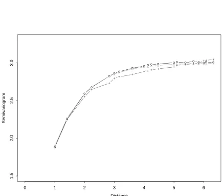
3.2 Average of 1000 empirical semivariograms for data on a 10 x 10 grid

generated from a constant mean process with an exponential (sill=1,range=3) semivariogram (∆): empirical semivariogram (O) and isotonized ver-sion (+). Standard deviations of estimates are approximately bounded

by .02. . . 18

3.3 Exponential(sill=1,range=3) semivariogram (∆) for data on a 10 by

10 grid, average of 1000 empirical semivariograms from residuals with

p= 3 estimated parameters (O) and with p= 6 estimated parameters

(+). Standard deviations of estimates are approximately bounded by

.02. . . 21

3.4 Exponential(sill=2,range=3) semivariogram (∆) on a 10 x 10 grid and

the average of 1000 replications of semivariogram estimates based on

residuals from p = 3 estimated parameters: empirical semivariogram

from residuals (O), bias-reduced empirical variogram (+), monotonized

bias-reduced empirical variogram (×). Standard deviations of

esti-mates are approximately bounded by .02. . . 24

3.5 Exponential(sill=1,range=3) semivariogram (∆), average of 1000

repli-cations of semivariogram estimates based on residuals from p = 3

es-timated parameters: empirical semivariogram from residuals (O) and weighted nonlinear least squares parametric estimate (+). Standard

deviations of estimates are approximately bounded by .02. . . 28

9.1 One dimensional tapering function with different values of a smoothing

parameter ρ. . . 61

9.2 The Multiplicative two dimensional tapering function. . . 62

(12)

Part I

Variance Estimation in Spatial

Regression Using a Nonparametric

Semivariogram Based on Residuals

(13)

Introduction

Random processes over time or space typically have the property that nearby

obser-vations tend to be more alike than obserobser-vations far apart. Scientific studies of such

processes often involve modeling and estimation of a mean response with random

errors assumed to be from a stationary process. For example, an additive error linear

model is given by

Yi =xTiβ+ei, i= 1, . . . , n, (1.1)

where xi may consist of variables that are a function of location as well as other

co-variates, and theei are errors whose correlation depends only on the distance between

observations.

One standard approach with normally distributed errors is to assume a particular

parametric semivariogram model such as an exponential and use restricted

maxi-mum likelihood (REML) for estimating the parameters of the model and then to

use estimated generalized least squares (EGLS) for estimating β. Alternatively, one

can avoid the normality assumption and use weighted least squares with the

empir-ical semivariogram of the residuals to estimate the parameters of the semivariogram

(14)

Chapter 1. Introduction 3

model (see Cressie, 1993, p. 94-99, 165-170). In either case the variance of the EGLS

b

β is estimated using standard formulas for generalized least squares with

semivari-ogram estimates inserted where needed. A correct semivarisemivari-ogram model, however,

is not always easy to choose, and we may be interested in estimation methods other

than least squares.

The purpose of this paper is to give new methods for estimating the variance of

b

β when βb is obtained from a general estimating equations approach, i.e., satisfying

P

Si(Yi,xi,β,b σb) =0, where Si is usually a function of residuals and weights andσb

are additional dispersion parameter estimates. This general class includes ordinary

least squares (OLS, with Si(Yi,xi,β,b σb) = (Yi−xTi βb)xi), EGLS, robust regression

(e.g., Huber, 1980, Ch. 3, with Si(Yi,xi,β,b σb) = (ψ[Yi−xTi βb]/bσ)xi), and

general-ized estimating equations (GEE, Liang and Zeger, 1986). Although these estimation

methods are suitable for a much larger class of models than (1.1), we will focus on

methods for (1.1). However, a parametric semivariogram model will not be chosen;

rather, we will estimate the semivariogram subject only to a monotonicity constraint.

Our approach is similar in spirit to the that of Lumley and Heagerty (1999), who

use a weighted empirical variance estimate for the middle part of the “sandwich”

asymptotic variance formula that arises naturally from the estimating equations

for-mulation. Their approach is more general because it allows nonstationary errors; in

fact Lumley and Heagerty (1999) unify a variety of nonparametric methods including

(15)

and Yasui and Lele (1997). Related nonparametric methods are found in Carlstein

(1986), Sherman (1996), Sherman (1997), Garcia-Soidan and Hall (1997), and

Hea-gerty and Lumly (2000).

Our approach differs, though, in two ways from these other methods: we use

non-parametric semivariogram estimation for the middle part of the “sandwich,” and we

explicitly remove bias in the semivariogram estimates that would ordinarily result

from using residuals rather than errors (which are of course unknown). It is this

lat-ter bias issue that we feel is most important. Any nonparametric variance estimation

method based on residuals that does not address the bias issue is doomed to

under-estimate the variance of under-estimated coefficients and of predictions. The problem with

using residuals has long been recognized in the spatial statistics literature (Matheron,

1971, p. 152-155, and Cressie, p. 165-170). However, when fitting parametric

vari-ogram models, the bias is by definition not a problem for REML. It is also claimed

(see Cressie, 1993, p. 167-169) that the bias from residuals is not a major problem

when estimating parametric semivariograms by weighted least squares because the

early lags, where the bias in the empirical semivariogram is small, have the largest

weights (however, see Figure 5 of Section 3.2). In general, though, nonparametric

semivariogram methods will inherit the bias problem of the empirical semivariogram,

especially at moderate to large distances between observations (see Figure 3 in Section

(16)

3.2, but Matheron (1973) and Cressie (1987) propose a method similar to

differenc-ing in time series for handldifferenc-ing the bias issue. For visual confirmation of parametric

variogram models, Brownie and Gumpertz (1997) suggest adjusting REML estimates

of parametric semivariograms so that graphically they are aligned with a plot of the

empirical semivariogram of residuals.

Our nonparametric semivariogram is based on several simple ideas. First we

construct a semivariogram estimator in the constant mean case by monotonizing

the standard empirical semivariogram (see Section 3.1). We also check for

positive-definiteness and modify our estimate if it is not positive-definite. Next (Section 3.2)

we compute the bias of the residuals-based empirical variogram in model (1.1) when

β is estimated by OLS. Then we correct for this bias by multiplying the empirical

semivariogram by estimated factors computed at each distinct distance between

ob-servations. Finally, we monotonize and make positive-definite the adjusted empirical

semivariogram. This nonparametric semivariogram is then used to estimate the

vari-ance of the estimated regression coefficients. Monte Carlo results for OLS estimates

are given in Section 4.1, and results for robust regression estimates are given in

Sec-tion 4.2. We begin in SecSec-tion 2 with a general explanaSec-tion of how to estimate the

(17)

Variance Estimation of Regression

Parameters

The estimating equations approach provides a general framework for deriving the

asymptotic distribution of βb that solves

Gn(β) =

1

n n

X

i=1

Si(Yi,xi,β) =0

(and here for simplicity we have dropped the extra dispersion parametersσmentioned

in the Introduction). That is, by Taylor series approximation,

0=Gn(βb)≈Gn(β) + ˙Gn(β)(βb−β) +Rn,

where

˙

Gn(βb) = ∂

∂βTGn(β) =

1

n n

X

i=1

∂

∂βTSi(Yi,xi,β).

Then, under suitable regularity conditions,βb −→p βandβbis asymptotically normally

distributed with variance

A(β)−1B(β)A(β)−1 T = lim

n→∞[−E ˙Gn(β)]

−1 _Var[_G

n(β)]

n

[−E ˙Gn(β)]−1

oT

, (2.1)

(18)

Chapter 2. Variance Estimation of Regression Parameters 7

where it is assumed that there are matrices A(β) and B(β) such that −E ˙Gn(β) →

A(β) and nVar[Gn(β)] → B(β) as n → ∞. In likelihood models −E ˙Gn(β) =

nVar[Gn(β)] is the average Fisher information. The estimator

˙

Gn(βb) =

1 n n X i=1 ∂

∂βTSi(Yi,xi,

b

β)

will typically satisfy ˙Gn(βb)−E ˙Gn(β)

p

−→β even for correlated data.

Since we have a consistent estimator for E ˙Gn(β), the problem of finding a

con-sistent estimator of the asymptotic variance (2.1) is reduced to finding a concon-sistent

estimator for the middle term (times n),

nVar [Gn(β)] = E

" 1 n n X i=1 n X j=1

Si(Yi,xi,β)Sj(Yj,xj,β)T

#

.

Lumley and Heagerty (1999) point out that the empirical estimator

1 n n X i=1 n X j=1

Si(Yi,xi,βb)Sj(Yj,xj,

b

β)T = 1

n

" _n X

i=1

Si(Yi,xi,βb)

# " _n X

j=1

Sj(Yj,xj,

b

β)T

#

is identically zero by the definition of βb. This of course contrasts with the common

situation where one can average over independent replications. Thus Lumley and

Heagerty (1999) suggest estimating the middle term by

b

Jn(βb) =

1 n n X i=1 n X j=1

wijnSi(Yi,xi,βb)Sj(Yj,xj,βb)T

where wijn → 1 as n → ∞ but wijn → 0 as the distance between two locations,

d(i, j)→ ∞for fixedn. They also show that the methods proposed earlier by Newey

(19)

as weighted empirical estimators with different choices of the weight wijn. Although

these estimators can be used for nonstationary models, one common problem is that

they are not very efficient for highly correlated data (Andrews, 1991).

To implement our approach we first make the simplifying assumption thatSi has

the form Si(Yi,xi,β) =wi(β)S(ei(β))xi, where S is now a real-valued function and

theei(β) are from a stationary process. Thus, theS(ei(β)) are also from a stationary

process, and we will estimate the latter process using semivariogram techniques. We

then employ it to estimate the middle term of (2.1) utilizing the relationship between

semivariogram and covariance functions under second-order stationarity. We present

(20)

Chapter 3 Nonparametric Semivariogram Estimation

A process {Z(s),s ∈ D, D ⊂ R

d_}

is called intrinsically stationary when it has

con-stant expectation and the variance of the increments depends only on the difference

of locations. For an intrinsically stationary process, the semivariogram is defined as

γ(s1 −s2) = 1

2Var[Z(s1)−Z(s2)].

It is called isotropic ifγ(s1−s2) is only a function of the Euclidean distanceks1−s2k

between locations. We then use the simpler notation γ(h) where h is the distance

between locations. The function 2γ(·) is called the variogram. A valid semivariogram

needs to be conditionally negative-definite; that is, it must satisfy

n

X

i=1

n

X

j=1

λiλjγ(si−sj) ≤0

for each set of locationss1, ...,snand allλ1, . . . , λnsuch that

Pn

i=1λi = 0 (see Cressie,

1993, p. 86). For a sample of given realizations fromZ(·), the empirical variogram is

(21)

the unbiased estimator of an isotropic variogram given by

2bγ(h) = 1

|N(h)|

X

N(h)

{Z(si)−Z(sj)}

2

where

N(h) ={(si,sj) :ksi−sjk=h:i, j = 1,2, ..., n}

and|N(h)|is the number of distinct pairs in N(h). Although the empirical variogram

is unbiased for the variogram, it cannot be used directly in procedures such as kriging

(spatial prediction) because it may not be negative-definite.

One standard approach has been to choose a parametric variogram model (which

by definition is negative-definite) and fit it by restricted maximum likelihood (REML),

maximum likelihood (ML), or weighted nonlinear least squares. There are a number

of widely used parametric variogram models based on isotropic processes such as the

exponential, spherical, and Gaussian. The Mat´ern class, originally given by Mat´ern

(1960), allows a wide range of flexibility in that it has a parameter which controls the

smoothness of a random field. The class can be defined by its isotropic autocovariance

function:

C(h) = σ

2ν−1_Γ(_ν₎

2ν1/2_h

ρ

ν

Kν

2ν1/2_h

ρ

whereσ is the scale parameter,ρthe range parameter, and ν is the shape parameter.

The function Γ(·) is the gamma function and Kν is the modified Bessel function

of the third kind of order ν (Stein 1999). When ν = 1₂, the model becomes the

(22)

Chapter 3. Nonparametric Semivariogram Estimation 11

underlying true variogram is rarely known, and selection of a variogram model is

quite arbitrary in practice. The Mat´ern class appears to be the best choice of the

present parametric models to estimate the dependence structure of a process since it

includes or approximates a number of common models.

3.1 Previous Methods

There have been several attempts to avoid selecting variogram models via

nonpara-metric variogram estimation (Shapiro and Botha, 1991; Cherry et al., 1996; S. Lele,

1995; Hall et al, 1994; Barry and Ver Hoef, 1996; and Gorsich and Genton, 1999).

Shapiro and Botha(1991) appear to be the first to consider a nonparametric

semivar-iogram estimate based on Bochner’s theorem. Cherry et al. (1996) implemented the

Shapiro-Botha estimator using the statistical package S-plus and compared its

perfor-mance to parametric estimation of the semivariogram using non-linear least squares.

They found good performance of their nonparametric estimates and sometimes

bet-ter performance than the traditional parametric approach. One problem with their

method is that the sill estimates tend to be biased and highly variable. Cherry (1996)

suggested a simple remedy for this sill problem, but semivariogram values other than

the sill also seem to have high variability as well. Lele (1995) provided a

nonparamet-ric estimator of the semivariogram using a spline function and included a study of the

performance of his estimator in terms of prediction and prediction error. However,

(23)

3.1.1 Method Proposed by Shapiro and Botha

Their method is based on Bochner’s theorem (Schoenberg 1938): A function f is

continuous and nonnegative definite if and only if it is the Fourier transform of a

nonnegative bounded Borel measure µ, i.e.

f(h) =

Z _∞

0

Ωd(ht)dF(t),

where F(t) is a non-decreasing bounded function on t ≥ 0 and Ωd(ht) is a basis for

functions in R

d _{having the form}

Ωd(x) = (2/x)(d−2)/2Γ(d/2)J(d−2)/2(x)

whereJv(d) is a Bessel function of the first kind of orderv. In the one, two and three

dimensional cases Ω1(x) = cos(x), Ω2(x) =J0(x), and Ω3(x) = sin(x)/x.

Using the identity, γ(h) =C(0)−C(h) for a second-order stationary process with

covariance function C(h), c0−f(h) for any constant c0 is continuous, conditionally

negative definite, and a valid semivariogram function. Then, the fitting of such valid

functions to the empirical semivariogram can be accomplished using weighted least

squares.

To solve the estimation problem numerically, let F(t) be a step function with m

finite positive jumps p1, ..., pm at points t1, ..., tm. Then F(t) can be expressed as

(24)

nonparametric semivariogram estimate can be expressed as:

ˆ

γ(hi) = m

X

j=1

pj(1−Ωd(hitj))

wherei= 1, ..., lis the lag number. The corresponding sill estimate is ˆC(0) =Pm_i₌₁pj.

The weighted least squares estimation problem can be formulated as follows: find a

m×1 vector p= (p1, ..., pm) that minimizes

Q(p) =

l

X

i=1

wi{ˆγ(hi)− m

X

j=1

pj(1−Ωd(hitj))}2.

3.1.2 Nonparametric Semivariogram Estimation by Lele

Lele proposed a method that transforms the problem of estimation of the valid

semivariogram matrix to the problem of estimation of the valid inner product

semi-variogram matrix. Simple smoothed semisemi-variograms (i.e. smoothed scatter plot of

(z(si)−z(sj))

2 _{using kernel functions or splines) can be considered as nonparametric}

semivariogram estimates, but these would violate the conditionally negative definite

property of valid semivariograms. However, it is comparatively easier to approximate

any finite dimensional matrix with a positive definite matrix than using the class

of conditionally negative definite functions (Shapiro and Botha, 1991; Cherry, 1994;

Hall, Fisher, and Hoffman, 1994): Write the spectral decomposition of a matrix Ψ

using the eigenvalues and eigenvectors of Ψ (i.e. Ψ = P DPT where P is the

ma-trix of eigenvectors and D consists of eigenvalues for diagonal elements and of zeros

(25)

number and denote this by D∗. ˆΨ = P D∗PT is an approximate positive definite matrix estimate of Ψ. Lele’s estimator is based on a spline smoother evaluated at a

finitely many points and these points are approximated by a collection of

condition-ally negative definite values. The approximated values are then smoothed by a spline

smoother again and these steps are repeated until the spline smoother and the spline

interpolator get nearly identical.

Steps to obtain Lele’s nonparametric semivariogram estimator: 1. Compute the empirical semivariogram estimates.

2. Smooth the empirical semivariogram using a spline function.

3. Obtain the spline-smoothed empirical semivariogram values, ˜γ’s, for all distances

and compute the corresponding inner product semivariogram values, Ψij’s, utilizing

the relationship:

˜

Ψij = ˜γi1+ ˜γj1−˜γij.

Note that the variance-covariance matrix,Ψ, of the vector of contrastsZcis called the

inner product semivariogram matrix.

4. Construct the variance-covariance matrix(Ψ) of the vector of contrasts, Zc =

(Z(s2)−Z(s1), Z(s3)−Z(s2), ..., Z(sn)−Z(s1)),and obtain the approximate positive

definite covariance matrix, ˆΨ.

5. Obtain the spline-interpolated semivariogram estimates, ˆγij’s from ˆΨij using the

relationship:

(26)

6. Plot the ˆγij’s against all distances ksi−sjk.

7. Repeat steps 2-5 until the resultant plot is visually smooth.

3.2 Monotone Semivariogram Estimation

Most parametric covariance models used in time series and spatial analyses have

cor-relations that are monotone decreasing with distance. Moreover, most physical

pro-cesses exhibit this monotone behavior as well. Thus, the centerpiece of our approach

is to assume that the correlations are momotone decreasing with distance. This is a

much weaker assumption than any of the common parametric semivariogram models.

Our basic approach to produce a nonparametric monotone semivariogram

esti-mator is to apply the pool adjacent violators algorithm (PAVA, Barlow et al. 1972,

p.13) to empirical semivariogram estimates. Although the variance of the empirical

semivariogram at a lag h is not exactly proportional to the inverse of the number of

pairs (e.g., Genton, 1998, p. 328), we will use that weighting in the PAVA routine.

This is similar to Cressie’s (1993, p. 96) weighting in nonlinear least squares fitting of

parametric semivariograms except that for simplicity we ignore the extra weighting

factor due to the value of the semivariogram.

The basic idea of PAVA is the following (using equal weights for simplicity):

start-ing with y1, move to the right and stop if yi > yi+1. In that case replace yi and yi+1

by their weighted average y∗_i =y_i∗₊₁ = (yi +yi+1)/2. Then move to the left to make

sure that yi−1 ≤ y∗i. If yi−1 > y∗i, then replace yi−1 with the weighted average of all

(27)

proceed again to the right. This process of averaging and back-averaging is continued

until the right end point is reached. In many situations, isotonic estimators have

improved mean squared error properties over the original estimators used in their

construction. We will illustrate that property with Monte Carlo simulation.

Since the variance of the empirical semivariogram is large for large lags, we follow

the common practice of truncating the isotonized semivariogram at half the maximum

distance found in the data set. In order not to induce upward bias at that distance,

we monotonize a larger set of lags before truncating. For example, for a time series

on the equally spaced time points of 1, . . . ,100 we monotonize on the lags 1, . . . ,70

and then truncate at 50.

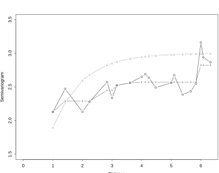
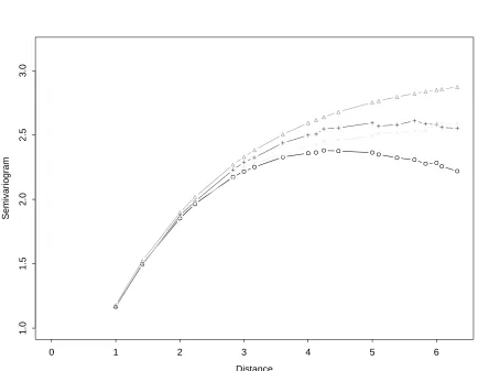
Figure 1 shows the empirical variogram and the isotonized semivariogram for one

data set on a 10 x 10 grid generated from an exponential semivariogram with range

parameter = 1 and sill = 3, γ(h) = 3[1−exp(−h/3)].

Figure 2 gives averages of 1000 replications of the situation in Figure 1. We can

see that the emprical variogram is unbiased as advertised, and that the monotone

estimate is somewhat biased downward in the middle. Table 1 shows, however, that

the monotone estimate has lower mean squared error for distances beyond 3. Note

that the standard errors of differences of estimates in Table 1 are lower than the

(28)

Distance

Semivariogram

0 1 2 3 4 5 6

1.5

2.0

2.5

3.0

3.5

(29)

Distance

Semivariogram

0 1 2 3 4 5 6

1.5

2.0

2.5

3.0

(30)

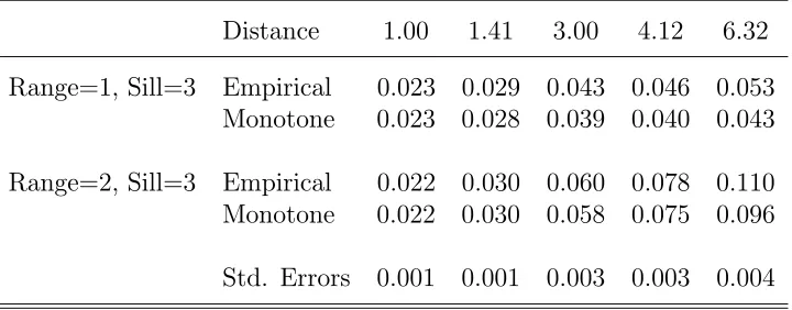
Table 3.1: Mean squared errors of the logarithm of empirical and monotone

semi-variogram estimates for constant mean data on a 10 × 10 grid with exponential

semivariogram. Results based on 1000 replications. Average standard errors are in the last row.

Distance 1.00 1.41 3.00 4.12 6.32

Range=1, Sill=3 Empirical 0.023 0.029 0.043 0.046 0.053

Monotone 0.023 0.028 0.039 0.040 0.043

Monotone 0.022 0.030 0.058 0.075 0.096

(31)

Very often, the isotonized semivariogram is already conditionally negative definite.

Sometimes it is not, and then we suggest using the spectral decomposition of the

co-variance matrix followed by replacement of the negative eigenvalues by small positive

ones. For the variance estimation discussed in Sections 4 and 5, this has virtually

no effect. However, for other purposes such as kriging, it may be required. Also,

the isotonic estimators have a “boxy” appearance, and sometimes we find it more

appealing to smooth the isotonized semivariogram using a spline or other smoother.

3.3 Bias Correction of Residuals-Based Variogram

Consider model (1.1) where the errors ei are drawn from a mean zero, second-order

stationary random error process. We shall assume that the unknown regression

co-efficients β are estimated by ordinary least squares. A natural approach is then to

c onstruct the empirical semivariogram from the residuals. Unfortunately, the

distri-bution of the residuals is not the same as the errors, and the empirical semivariogram

is seriously biased downward. Figure 3 shows the average of the empirical

semivar-iogram for 1000 replications of an exponential semivarsemivar-iogram with range parameter

= 1 and sill = 3 for a 10 by 10 grid. The middle line is for residuals based on fitting

an intercept and the location coordinates (x and y). The lower line is for residuals

from a fit with the same three variables and with three more independent variables

(32)

Distance

Semivariogram

0 1 2 3 4 5 6

1.5

2.0

2.5

3.0

Figure 3.3: Exponential(sill=1,range=3) semivariogram (∆) for data on a 10 by 10

grid, average of 1000 empirical semivariograms from residuals with p = 3 estimated

parameters (O) and with p = 6 estimated parameters (+). Standard deviations of

(33)

To understand more clearly the effect of the residuals, let V denote the covariance

matrix of the errors for a sample with ndata points. Then simple calculations show

that the covariance matrix of the residuals bei =Yi−xTi βis given by (I−P)V(I−P),

whereI is thendimensional identity matrix andP =X(XTX)−1XT is the projection

matrix of X, whereX is formed from the row vectors xT

i .

The expected value of the empirical semivariogram of the residuals at lagh is

Eres(h) =

1

2|N(h)|

X

N(h)

E(bei+h−bei)2

= 1

2|N(h)|

X

N(h)

E(be2_i₊_h) + E(be2_i)−2E(bei+hbei)

≈ 1

ntrace(I−P)V(I−P)−

1

|N(h)|

X

N(h)

[(I−P)V(I −P)]_i,i₊_h,

where the approximation comes in by taking the average of all of the diagonal elements

of (I−P)V(I−P) instead of the subset of the diagonal elements implied by summing

over elements h distance apart. This approximation is not necessary but makes the

computing considerably easier.

The expected value of the empirical variogram of the errors at lag h is of course

γ(h), but we can write it in a form similar to the above:

Eerr(h) =

1

2|N(h)|

X

N(h)

E(ei+h−ei)2

= σ2− 1

|N(h)|

X

N(h)

(34)

where σ2 is the variance of the errors. Now the ratio of these quantities, fac(h) =

Eerr(h)/Eres(h), is essentially the ratio of the true semivariogramγ(h) in Figure 3 to

the average of the empirical semivariograms.

We feel that the downward bias in Figure 3 in unacceptable. Moreover,

apply-ing PAVA to the residual-based empirical semivariogram will certainly improve it,

but the scope for improvement is quite limited. Thus we feel it is important to first

adjust the empirical semivariogram before monotonizing. Our approach then is to

es-timate fac(h) by using estimated covariances obtained from the monotonized version

of the residual-based empirical semivariogram. We multiply these estimated factors

times the original residual-based empirical semivariogram resulting in a bias-reduced

empirical semivariogram. Finally we monotonize this bias-reduced empirical

semi-variogram to obtain our estimated semisemi-variogram. It is also possible to iterate the

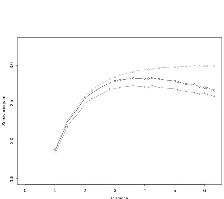
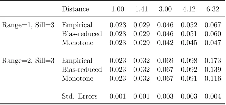
factor estimation step, but we found that it did not make much difference. Figure

4 shows the average of the residual-based empirical semivariogram, the bias-reduced

empirical semivariogram, and the monotonized version for 1000 samples from a linear

model with intercept and locations fitted (p= 3 case) and errors generated from an

exponential semivariogram with range parameter = 2 and sill = 3. Comparing Figure

4 with Figure 2, one can see that montonizing has a similar effect; that is, it tends to

(35)

Distance

Semivariogram

0 1 2 3 4 5 6

1.0

1.5

2.0

2.5

3.0

Figure 3.4: Exponential(sill=2,range=3) semivariogram (∆) on a 10 x 10 grid and the average of 1000 replications of semivariogram estimates based on

residu-als from p = 3 estimated parameters: empirical semivariogram from residuals (O),

bias-reduced empirical variogram (+), monotonized bias-reduced empirical variogram

(36)

Table 3.2: Mean squared errors of logarithms of semivariogram estimates:empirical,

bias-reduced empirical and monotone. Data are from a 10×10 grid with exponential

semivariogram. Results based on 1000 replications. Average standard errors are in the last row.

Distance 1.00 1.41 3.00 4.12 6.32

Bias-reduced 0.023 0.029 0.046 0.051 0.060

Monotone 0.023 0.029 0.042 0.045 0.047

Bias-reduced 0.023 0.032 0.067 0.092 0.139

Monotone 0.023 0.032 0.067 0.091 0.116

(37)

Table 2 shows that the monotonized version has improved mean squared error

properties relative to the original residual-based empirical semivariogram. Note that

the bias-reduced empirical semivariogram has increased mean squared error on the

larger distances. It is often the case that reducing bias is accompanied by increased

mean squared error. Fortunately, monotonizing leads to improved results.

A number of authors (see Cressie, 1993, p. p. 167-169) have shown concern about

the bias problems when the variogram is based on least squares residuals. However,

to our knowledge, no methods have successfully corrected the bias of residuals-based

empirical variograms. In general, the bias of such estimators is small at lags near

the origin but more substantial at distant lags (see Figure 3). Cressie (1993, p.

167-168) concludes that the effect of bias on kriging will be small if a parametric

variogram is fitted with more weight given to the estimates at small lags, such as by

the weighted least squares method. However, he notes that a kriging variance can be

more influenced by the residuals-based variogram estimates. Here our main concern

is with estimation of the variance of estimated regression parameters, not prediction,

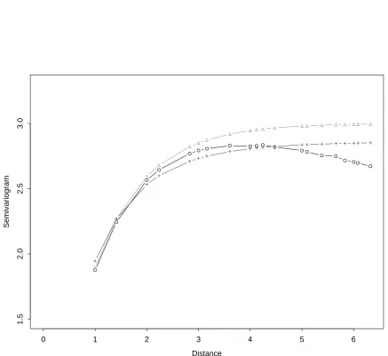
and the substantial bias at large lags should not be ignored. Figure 5 shows that

a parametric variogram estimated by WNLS fitted to the residual-based empirical

semivariogram has considerable bias.

The estimation approach least likely to be affected by residual bias is restricted

maximum likelihood (REML). REML maximizes the likelihood of error contrasts

(38)

REML method provides highly efficient and much less biased estimation compared

to regular maximum likelihood method, especially when the number of parameters

is large relative to the number of observations. The REML method is a useful tool

for analyzing data with spatial variation since it does not suffer from the often severe

underestimation of the parameters that ML does and produces less biased estimates.

One disadvantage of likelihood estimation procedures is that they rely heavily

on the Gaussian assumptions, and such assumptions are often inappropriate; the

underlying distribution of the most processes is not known or contamination of the

distribution can occur by a few errant observations. Nonparametric estimation of

the variogram may provide less sensitive estimates for some non-Gaussian models.

Of course, least squares estimation of regression coefficients is also questionable in

the face of non-Gaussian errors. In Section 5 we consider using robust regression

estimates.

For confirmation of parametric semivariogram models, Brownie and Gumpertz

(1997) suggest adjusting parametric semivariograms fitted by REML so that plots

of the adjusted semivariograms will be consistent with the residual-based empirical

semivariogram. Their approach is similar in spirit to our bias-reduced empirical

semivariogram; the difference is they adjust the fitted semivariogram instead of the

(39)

Distance

Semivariogram

0 1 2 3 4 5 6

1.5

2.0

2.5

3.0

Figure 3.5: Exponential(sill=1,range=3) semivariogram (∆), average of 1000

repli-cations of semivariogram estimates based on residuals from p = 3 estimated

(40)

Chapter 4 Variance Estimation of Regression

Parameters Based on Semivariograms

4.1 Ordinary Least Squares Estimates of

β

Under the model (1.1) with second order stationary errors and β estimated by

ordi-nary least squares, the variance of βb is given by

Var(βb) = (XTX)−1XTV X(XTX)−1,

whereV is the covariance matrix of the errors. For estimating this variance, we utilize

the relationship between a semivariogram function γ(h) and a covariance function

C(h) under second-order stationarity, γ(h) = C(0) −C(h) and C(h) = γ(∞)−

γ(h), where C(0) =γ(∞) is the variance of the errors. Then we use the monotone

semivariogram estimates proposed in Section 3.2 to estimate V and substitute in the

(41)

above expression.

Recall, though, that Figure 4 shows how the correlations tend to be overestimated

by our monotone semivariogram estimate. This happens because on average in the

middle distances the monotone estimate is biased downward. On a sample by sample

case, this can be seen when the middle part of the monotone estimate is flat but rises

near the half maximum distance. In such a case, the correlations are positive for a

large number of distancesh. This results in variance estimates that can be too large.

Thus we use a cutoff rule for correlations: we set any estimated correlation to 0 if

its value is smaller than 0.1/√n. This is a fairly arbitrary rule, but it is similar in

spirit to the WEAVE weight functions of Lumley and Heagerty (1999). Basically,

the number of nonzero correlations cannot be growing too quickly withnif we are to

have good variance estimates.

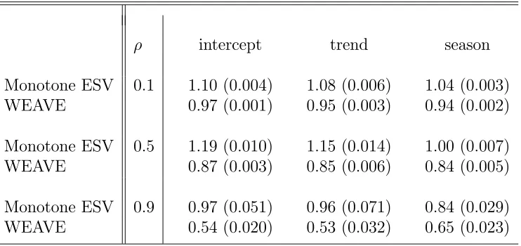
Table 4.1 shows results for errors from an ar(1) process with ρ =.1, .5., and .9.

The X matrix consists of an intercept term, a linear trend, and a seasonal term and

was taken from the simulation study of Lumley and Heagerty (1999, p. 469). For

comparison, we also report results using the approach of Lumley and Heagerty (1999)

denoted by “WEAVE” in Table 3. We obtained their results using a program from

their website with default values. Perhaps other settings would have performed better

for theρ=.9 case. Our results, denoted by “Monotone ESV” for monotone empirical

semivariogram, are reasonably on target (values close to 1.00), but more variable than

(42)

Chapter 4. Variance Estimation of Regression Parameters Based on Semivariograms31

Table 4.1: Average of Standard Deviation Estimates (divided by true standard deviation) for Regression from Time Series Data of Size 100 with Autoregressive Errors. Based on 100 replications. Standard errors are in parentheses.

ρ intercept trend season

Monotone ESV 0.1 1.10 (0.004) 1.08 (0.006) 1.04 (0.003)

WEAVE 0.97 (0.001) 0.95 (0.003) 0.94 (0.002)

Monotone ESV 0.5 1.19 (0.010) 1.15 (0.014) 1.00 (0.007)

WEAVE 0.87 (0.003) 0.85 (0.006) 0.84 (0.005)

Monotone ESV 0.9 0.97 (0.051) 0.96 (0.071) 0.84 (0.029)

(43)

our estimates are larger on average than the WEAVE estimates.

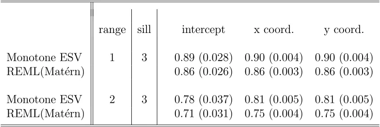
Table 4.2 shows results for Gaussian spatial processes observed on a 10 ×10

grid, that are generated using an exponential variogram model with the sill = 3

and range parameter = 1 and 2, respectively. The average correlation is 0.04 for

the model with the range parameter equal to 1, and is 0.14 for the model with

the range parameter 2. (For comparison with the time series simulation in Table

3, note that the average correlation for ρ = .1, .5, and .9 are .002, .02, and .16,

respectively.) A mean surface was added to these Gaussian processes to describe

a spatial trend: f(µ) = β0 +β1x +β2y, where (x, y) defines a point in R

2 _with

β0 = 0.0, β1 = 0.9, β2 = 0.06. Three covariates, a column of ones for the intercept

and x (longitude) and y (latitude), were fitted to the model to estimate the mean

surface. We then compared our methods to REML estimation using an assumed

Mat´ern variogram model (which is correct here). We see in Table 4 that our estimates

are a little closer to the target value and a little more variable than the REML-Mat´ern

estimates. Our estimates have one large advantage not illustrated by these results:

our approach is totally invariant to the presence or absence of a nugget effect. In

contrast, with a nugget effect the Mat´ern model would need to be fit with an added

nugget parameter and results then would be more variable.

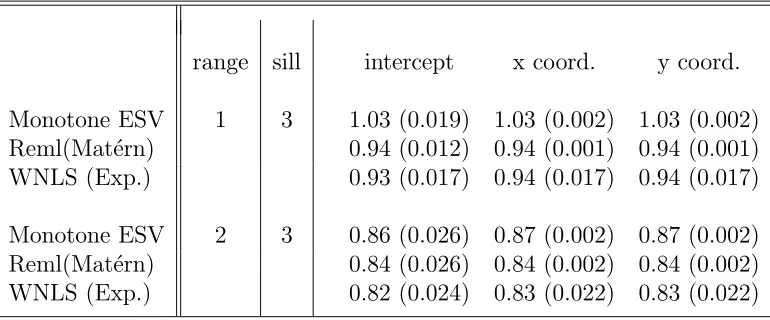
Table 4.3 contains results similar to Table 4.2 but for a 16 by 16 lattice. Comparing

Table 4.2 and Table 4.3 shows that performance is improving with sample size.

(44)

with smoothing parameter 1, often called the Whittle model (Whittle, 1954). Whittle

suggests that this model is natural for agricultural field trials. Results here are similar

(45)

Table 4.2: Average of Standard Deviation Estimates (divided by true standard

deviation) for Regression from 10×10 Spatial Data of Size 100 with Exponential

Variogram Errors. Based on 100 replications. Standard errors are in parentheses.

range sill intercept x coord. y coord.

Monotone ESV 1 3 0.89 (0.028) 0.90 (0.004) 0.90 (0.004)

REML(Mat´ern) 0.86 (0.026) 0.86 (0.003) 0.86 (0.003)

Monotone ESV 2 3 0.78 (0.037) 0.81 (0.005) 0.81 (0.005)

(46)

deviation) for Regression from 16×16 Spatial Data of Size 100 with Exponential

Variogram Errors. Based on 100 replications. Standard errors are in parentheses.

Monotone ESV 1 3 1.03 (0.019) 1.03 (0.002) 1.03 (0.002)

Reml(Mat´ern) 0.94 (0.012) 0.94 (0.001) 0.94 (0.001)

WNLS (Exp.) 0.93 (0.017) 0.94 (0.017) 0.94 (0.017)

Monotone ESV 2 3 0.86 (0.026) 0.87 (0.002) 0.87 (0.002)

Reml(Mat´ern) 0.84 (0.026) 0.84 (0.002) 0.84 (0.002)

(47)

deviation) for Regression from 16×16 Spatial Data of Size 100 with Whittle Variogram

Errors. Based on 100 replications. Standard errors are in parentheses.

Monotone ESV 1 3 1.10 (0.016) 1.08 (0.001) 1.08 (0.001)

Reml(Mat´ern) 0.98 (0.007) 0.96 (0.001) 0.96 (0.001)

WNLS (Exp.) 0.98 (0.013) 0.96 (0.012) 0.96 (0.012)

Monotone ESV 2 3 1.00 (0.023) 0.99 (0.002) 0.99 (0.002)

Reml(Mat´ern) 0.93 (0.015) 0.93 (0.001) 0.93 (0.001)

(48)

4.2 Robust Regression Estimates of

β

The OLS estimators minimize the sum of residual squaresPn_i₌₁ei(β)2, and effieciency

losses may arise since this sum of squares is sensitive to large values that occur

more frequently with non-Gaussian data. Robust M-estimators minimize an objective

function Pn_i₌₁ρ(ei(β)) that is less sensitive to large values. Equivalently by taking

derivatives, one solvesPn_i₌₁ψ(ei(β))xi = 0, whereψ =ρ0. In order for the estimators

to be scale invariant, one needs to alter the above equation to

n

X

i=1

ψ

ei(β)

b

σ

xi = 0,

where bσ is a scale estimate. There are different options for selecting ρ and bσ, but a

common approach is to use

ρ(t) =

       t2

2 if |t| ≤k,

k|t| −k₂2 otherwise.

ψ(t) =

              

−k if t < k, t if −k ≤t ≤k, k if t > k.

where k is a tuning constant, usually selected to give an appropriate asymptotic

(49)

b

σ by solving simultaneously

n

X

i=1

ψ2

ei(β)

b

σ

=Ck,

whereCkis a constant chosen so thatσbis consistent for the standard deviation when

the data are from a Gaussian distribution. For example, when k = 1, C1 =.516, and

the asymptotic relative efficiency ofβb to least squares for independent Gaussian data

is close to 90%.

Asymptotic normality of βb was proved by Koul (1977, p. 688). One version of

the asymptotic variance is given by

D(XTX)−1XTVψX(XTX)−1,

where D = σ/Eψ0(e1/σ) and Vψ is the covariance matrix of ψ(e1/σ), . . . , ψ(en/σ).

We should also mention that we have ignored the role of estimating σ in the

asymp-totic distribution of βb because for errors with symmetric marginal distributions, the

asymptotic correlation between βb and σb is zero.

These M-estimators fit into the general scheme outlined in Section 2. That is,

we assume that ψ(e1/σ), . . . , ψ(en/σ) are second-order stationary and estimate their

covariance matrix using our nonparametric semivariogram estimator based on

(50)

deviation) for Regression from 10×10 Spatial Data of Size 100 with t-transformed

Exponential Variogram Errors. Based on 100 replications. Standard errors are in

parentheses. True standard deviations are based on 10000 replications and have

estimated coefficient of variation .007.

r s intercept x coord. y coord.

True Stand. Dev. (LS) 1 3 0.84 0.118 0.118

True Stand. Dev. (Robust) 0.75 0.106 0.106

Monotone ESV (LS) 1 3 0.91 (0.036) 0.91 (0.034) 0.91 (0.034)

Monotone ESV (Robust) 0.89 (0.035) 0.90 (0.032) 0.90 (0.040)

True Stand. Dev. (LS) 2 3 1.25 0.168 0.168

True Stand. Dev. (Robust) 1.14 0.154 0.154

Monotone ESV (LS) 2 3 0.73 (0.031) 0.75 (0.031) 0.75 (0.031)

(51)

least squares residuals. However, one way to motivate their use is by defining

pseudo-observationsYei =xTiβb+dψ(bei/bσ) for any constantd. Then the least squares estimate

based onYei is just βb, and the residuals are dψ(bei/bσ).

Table 4.5 shows results for situations similar to Table 4.2 but with errors from t

-transformed exponential variogram models. That is, we -transformed the exponential

errors used in Table 4.2 using the transformation F₅−1(Φ(Yi/

√

3)), where Φ is the

standard normal distribution function andF₅−1 is the inverse distribution function of

a t distribution with 5 degrees of freedom. Thus the marginal distribution of Yi is a

t distribution with 5 degrees of freedom.

The entries in rows 1 and 2 and 5 and 6 of Table 4.5 are Monte Carlo estimates of

the variance ofβb based on 10,000 replications. These show that the robust regression

estimates have less variability than the least squares estimates as expected. The other

rows are our standard deviation estimates for the regression parameter estimates

divided by the estimated true standard deviations. The results are fairly similar to

Table 4.2 and show that the estimates are negatively biased but less biased for the

(52)

Chapter 5 Discussion

Our main goal has been to estimate the variance of regression coefficients obtained

from a general estimating equations approach without making parametric

semivari-ogram assumptions. Thus we have proposed a new method for nonparametric

semi-variogram estimation based on monotonizing a reduced-bias empirical semisemi-variogram

based on residuals.

The simulations of Section 4 indicate that the resulting variance estimates are

reasonably unbiased and are converging as the sample size grows. Comparison with

REML using the true Mat´ern model shows that the new method is competitive with

parametric methods. It would be useful to make comparisons when the true model is

not from the Mat´ern model.

(53)

Bibliography

Andrews, D.W.K. (1991), “Heteroskedasticity and Autocorrelation Consistent

Co-variance Matrix Estimation,” Econometrica, Vol. 59, No.3 817-858.

Barlow, R., Bartholemew, D., Bremner, J., and Brunk, H. (1972)Statistical Inference

Under Order Restrictions, John Wiley, New York.

Barry J.P. and Ver Hoef, J. M. (1996), “ Blackbox Kriging: Spatial Prediction

With-out Specifying Variogram Models,”Journal of Agricultural, Biological, and

Envi-ronmental Statistics, 3, 297-322.

Brownie, C. and Gumpertz, M. (1997), “Validity of spatial analyses for large field

trials,”Journal of Agricultural, Biological, and Environmental Statistics, 2, 1-23.

Carlstein, E. (1986), “The Use of Subseries Values for Estimating the Variance of

(54)

Chapter 6. Bibliography 43

a General Statistic from a Stationary Sequence,”The Annals of Statistics, 14,

1171-1179.

Cherry, S., Banfield, J., and Quimby, W.F. (1996), “An Evaluation of a

Nonpara-metric Method of Estimating Semi-variograms of Isotropic Spatial Processes,”

Journal of Applied Statistics, Vol. 23, No. 4, 435-449.

Cherry, S. (1997), “Non-parametric Estimation of the Sill in Geostatistics,”

Environ-metrics, 8, 13-27.

Cressie, N. (1987), “A Nonparametric View of Generalized Covariances for Kriging,”

Mathematical Geology, Vol. 19, 425-449.

Cressie, N. (1993), Statistics for Spatial DataJohn Wiley, New York.

Garcia-Soidan, P. H. and Hall, P. (1997), “On Sample Reuse Methods for Spatial

Data,”Journal of the American Statistical Association,Biometrics, 53, 273-281.

Genton, M. G. (1998) “Variogram Fitting by Generalized Least Squares Using an

Explicit Formula for the Covariance Structure,” Mathematical Geology, Vol. 30,

No. 4, 323-345.

Gorsich, D. J., and Genton, M. G.(2000) “Variogram Model Selection via

(55)

Hall, P., Fisher, N. I., and Hoffman, B. (1994), “On the Nonparametric Estimation

of Covariance Functions,” The Annals of Statistics, 22, 2115-2134.

Heagerty, P.J. and Lumley, T. (2000), “Window Subsampling of Estimating Functions

With Application to Regression Models,” Journal of the American Statistical

Association, 95, 197-211.

Huber, P. (1980),Robust Statistics John Wiley, New York.

Koul, H. L. (1977), “Behavior of Robust Estimators in the Regression Model with

Dependent Errors,” Annals of Statistics, 5, 681-699.

Lele, S. (1991), “Jackknifing Linear Estimating Equations: Asymptotic Theory and

Applications in Stochastic Processes,” Journal of the Royal Statistical Society,

Ser. B, 53, 253-267.

Lele, S. (1995), “Inner Product Matrices, Kriging, and Nonparametric Estimation of

the Variogram,” Mathematical Geology, 27, 673-692.

Liang, K.-Y., and Zeger, S.L. (1986), “Longitudinal Data Analysis Using Generalized

Linear Models,” Biometrika, 73, 13-22.

Lumley, T. and Heagerty, P.J. (1999), “Weighted Empirical Adaptive Variance

Esti-mators for Correlated data regression,” Journal of the Royal Statistical Society,

(56)

Chapter 6. Bibliography 45

Mat´ern, B. (1960), Spatial Variation. Meddelanden fran Stantens

Skogsforsknin-ingsinstitut, 49, No. 5.

Matheron, G. (1971), The Theory of Regionalized Variables and Its Applications,

Cahiers du Centre de Morphologie Mathematique, No. 5, Fontainebleau, France.

Matheron, G. (1973), “The Intrinsic Random Functions and Their Applications,”

Advances in Applied Probability, 5, 439-468.

Newey, W.K., and West, K.D. (1987), “A Simple Positive Semi-Definite,

Heteroskedas-ticity and Autocorrelation Consistent Covariance Matrix,”Econometrica, 55,

703-708.

Shapiro, A. and Botha, J.D. (1991), “Variogram Fitting with a General Class of

Con-ditionally Nonnegative Definite Functions,” Computational Statistics and Data

Analysis, 11, 87-96.

Sherman, M. (1996), “Variance Estimation for Statistics Computed from Spatial

Lat-tice Data,”Journal of the Royal Statistical Society, Ser. B, 58, 509-523.

Sherman, M. (1997), “Subseries Methods in Regression,” Journal of the American

Statistical Association, 92, 1041-1048.

(57)

White, H., and Domowitz, I. (1984), “Nonlinear Regression with Dependent

Obser-vations,” Econometrica, 52, 143-161.

Whittle, P. (1954), “On stationary processes in the plane,” Biometrika, 41, 434-449.

Yasui and Lele, S. (1997), “A Regression Method for Spatial Disease Rates: an

Esti-mating Function Approach,” Journal of the American Statistical Association, 92,

(58)

Part II

Spectral Analysis with Spatial

Periodogram and Data Tapers

(59)

Introduction

This part of the thesis proposes statistical methods for characterizing stationary

spa-tial processes in the spectral (frequency) domain. The analysis of stationary processes

with their spectral representations in the frequency domain is referred to as spectral

analysis. More familiar approaches to treating the data from spatial processes involve

studying and estimating the covariance function in the time-space domain. Further,

most standard results in spectral analysis have been established for one-dimensional

(time series) data. Our research is devoted to developing alternative approaches to

the conventional space domain methods, extending existing spectral domain results

for time series data to higher dimensional spatial data. Spectral analysis finds broad

applications in many branches of science such as Oceanography, Physics, Electrical

engineering, and Geostatistics. It is useful in a variety of practical problems including

interpretation of energy and frequency distributions of random periodic data,

predic-tion and filtering problems, and statistical model fitting of processes. It is particularly

(60)

advantageous in analyzing large data sets and in studying properties of multivariate

processes. Geostatistical data are usually collected over a large region, and handling

large data sets is often problematic for the commonly used techniques: for example,

inversion of a large covariance matrix to compute a likelihood function may not be

possible or may demand much effort and time in computation. The use of a Fast

Fourier Transform (FFT) algorithm, which is a key operation in spectral analysis,

can be a good resolution to these computing problems. However, the FFT can be

applied only to regularly spaced data, so data observed on an irregular grid need to

be digitized for FFT.

The spatial periodogram, which can be thought of as a counterpart to the

empiri-cal variogram, is a powerful tool to estimate the correlation structure of a stationary

process. It is a nonparametric estimate of the spectral density, which is the Fourier

transform of the covariance function. The properties of the spatial periodogram have

been investigated by Stein (1995), Guyon (1992, 1982), Ripley (1981), Rosenblatt

(1985) and Whittle (1954). The empirical variogram, which is the most widely used

in the time-space domain for estimating the dependence structure of data, is

usu-ally fitted to parametric variogram models using techniques such as non-linear least

squares (NLS) and restricted maximum likelihood (REML) methods. However, the

same data points are used to obtain the empirical variogram at different lags,

re-sulting in estimates which are more highly correlated than the data observations.

(61)

practice and one usually does not account for the correlation between them to fit a

variogram model. Ignoring such correlation can certainly mislead data analyses. On

the other hand, in the spectral domain the periodogram values at any set of Fourier

frequencies are asymptotically uncorrelated. The asymptotic independence of the

periodogram estimates gives one of the big advantages of spectral analysis in that

techniques such as NLS can be naturally applied without incorporating an estimated

correlation. However, the spatial periodogram itself is not a consistent estimator of

the spectral density. In order to achieve consistency, application of smoothing filters

directly to the periodogram estimates has been more considered in the past. The

edge-effect problem does not vanish even asymptotically when we smooth the spatial

periodogram in two or higher dimensions. For one-dimensional data, there is only

one boundary point at each end, but the number of boundary points increases with

the dimension, leading to more serious edge effects. Instead of smoothing biased

pe-riodogram estimates, filtering the raw data with a data taper before computing the

periodogram not only provides a consistent estimate of the spectral density but also

is highly effective in removing edge-effects. The information lost by smoothing the

periodogram because of the presence of powerful frequencies can be better recovered

by data tapers. Prewhitening is another method of filtering data to control the bias

of the periodogram. Moreover, with the fixed-domain asymptotic approach, where

the number of observations increases in a fixed study area, it has been shown that

(62)

(Stein, 1995).

The effect of tapering higher dimensional data in the space domain was studied by

Dalhaus and K¨unsch (1987), who examined the tapering effect for the usual sample

covariance estimator. In this thesis, we first propose to use the tensor product of two

one-dimensional tapering functions to filter the data before computing the spatial

periodogram. We present a method to choose an appropriate amount of smoothing

for data tapers, taking into consideration the tradeoff between the bias and variance

of the tapered periodogram. We also introduce a new asymptotic approach for spatial

data called ‘shrinking asymptotics’ which extends the idea employed for time series

data by Constantine and Hall (1994). In the shrinking asymptotic approach, we

consider decreasing the space between data observations, allowing the number of

observations to increase at the same time as we expand the studying area. This

approach enables us to avoid aliasing problems and to uniquely estimate the spectral

density.

In Section 2, we introduce the spatial periodogram which is generalized from the

traditional one-dimensional periodogram in time series analysis. In Section 3, the

properties of tapering functions are briefly described. A method of estimating the

spectral density with the tapered spatial periodogram based on shrinking asymptotics

is given in Section 4. Lastly, the practical method to choose an appropriate amount

of smoothing for spatial data is proposed based on the study of the asymptotic mean

(63)

Spatial Periodogram

8.1 Spectral Representation of a Stationary

Ran-dom Field

A random field is weakly stationary if its expectation and variance are both translation

invariant over the domain.If a random field Z(x), x∈R

2_{, is weakly stationary then}

it can be represented as

Z(x) =

Z

R

2 exp(iλ

T_x₎_dφ₍_λ₎_,

where φ(λ) is an orthogonal-increment process (i.e. the process φ(λ) has the special

property that its increments at different values of λ are uncorrelated). The process

(64)

Chapter 8. Spatial Periodogram 53

φ(λ) and a stationary random field Z(x) are related in the following way

E[|φ(λ)|2] =F(λ),

whereF(λ) is a positive finite measure called a spectral distribution function. Priestly

(1996) describes the spectral representation of a stationary process as follows:

“This spectral representation of the process Z(x) essentially tells us that any

stationary process can be represented as the limit of the sum of sine and cosine

functions with random coefficients dφ(λ), or more precisely, with random amplitudes

|dφ(λ)| and random phases arg{dφ(λ)}.”

The covariance function CZ(x) = Cov{Z(x+u), Z(u)}, assuming zero mean for

Z(x), can be expressed in terms of the spectral measure F(·):

CZ(x) =

Z

R

2

exp(iλTx)F(dλ),

where F(·), a finite positive measure.When F(·) is differentiable with respect to

Lebesgue measure, the spectral density at frequencyλis defined as simply the Fourier

transform of the autocovariance function CZ(·):

fZ(λ) =

1

(2π)2

Z

R

2 exp(−iλ T

x)CZ(x)dx.

(65)

that obtained from its autocovariance.

8.2 Overview - Periodogram for Time Series Data

The periodogram was first introduced by Schuster (1898) as a tool to identify hidden

periodicities. The periodogram, which is a non-parametric estimate of the spectral

density, reflects periodic behavior of a time series and is a useful tool to analyze

stochastic processes. Smooth series are characterized by periodogram values which

have most of their power at low frequencies, whereas quickly oscillating series are

characterized by periodogram values which have most of their power at high

frequen-cies.

For a real-valued time series process, X(t), t = 0,±1, ... with mean E(X) and

autocovariance function CX(u), the spectral density of period 2π for the series X(t)

is defined as

fX(λ) =

1

2π

∞

X

u=−∞

CX(u)e−iλu, − ∞< λ <∞,

if

∞

X

u=−∞

|CX(u)|<∞,

CX(u) = Cov{X(t +u), X(t)}, t, u = 0,±1, .... To estimate the spectral density

fX(λ), we first compute the finite Fourier transform of the seriesX(t),

PT−1

t=0 X(t)e−

iλt_,

at a discrete set of frequencies. This finite Fourier transform is asymptotically

Nonparametric Spatial analysis in spectral and space domains

AND SPACE DOMAINS

Dedication

Acknowledgements

Table of Contents

I

Variance Estimation in Spatial Regression Using a

Non-parametric Semivariogram Based on Residuals

1

II

Spectral Analysis with Spatial Periodogram and Data

Tapers

47

List of Tables

Part I

Variance Estimation in Spatial

Regression Using a Nonparametric

Semivariogram Based on Residuals

Introduction

Variance Estimation of Regression

Parameters

Chapter 3

Nonparametric Semivariogram Estimation

3.1

Previous Methods

3.1.1

Method Proposed by Shapiro and Botha

3.1.2

Nonparametric Semivariogram Estimation by Lele

3.2

Monotone Semivariogram Estimation

3.3

Bias Correction of Residuals-Based Variogram

Chapter 4

Variance Estimation of Regression

Parameters Based on Semivariograms

4.1

Ordinary Least Squares Estimates of

β

4.2

Robust Regression Estimates of

β

Chapter 5

Discussion

Bibliography

Part II

Spectral Analysis with Spatial

Periodogram and Data Tapers

Introduction

Spatial Periodogram

8.1

Spectral Representation of a Stationary

Ran-dom Field

8.2

Overview - Periodogram for Time Series Data