Abstract
MEI, HAO. Novel Methods for Mapping Complex Disease. (Under the direction of Dr. Eden R. Martin).
In contrast to simple disease (or Mendalian disease), complex disease has its
spe-cial challenging characteristics for mapping. First, complex disease generally does
not have clear pattern of inheritance. Second, high-order interaction often occurs
in complex disease, where variants are widely assumed to be common (Common
Disease/Common Variants assumption) with only small or modest effects of each
variants. Third, genetic effects are often heterogeneneous, where different affected
individuals may attribute disease to different sets of causative genes. These
charac-teristics cause low power of mapping complex disease gene using linkage and tradtional
association methods,which motivated us to develop powerful novel methods with high
computational efficiency.
The first method extended the traditional method of Multifactor Dimensionality
Reduction (EMDR) to detect high-order interaction by finding significant multi-locus
models. EMDR does not assume any pattern inheritance. It applies the technique
of dimension reduction and the goodness-of-fitness test in the whole data to measure
association from a multi-locus model by χ2 statistic. This procedure is called
non-crossvalidation in contrast to 10-fold crossvalidaiton by MDR. The significance of the
χ2 statistic is tested by a non-fixed permutation procedure in contrast to the omnibus permutation procedure by MDR. By testing data from Genetic Analysis Workshop 14
(GAW14) with known answers, it was shown that EMDR with non-crossvalidation
and non-fixed permutation is more powerful than MDR without increasing type I
error. In addition, the computationally high efficiency of the EMDR program makes
it possible to analyze a large number of markers simultaneously.
However, EMDR does not consider genetic heterogeneity,which could decrease an
association signal in the data. The second method, MDR-Phenomics, is developed by
integrating phenotypic information in the analysis of EMDR. Since genetic
heterogeneity can be controlled by analyzing phenotypic covariate. MDR-Phenomics
classifies data into different groups based on discrete levels of a phenotypic covariate.
The different association across classified groups is measured by an F statistic from the ANOVA method. A new M statistic measuring association from a multi-locus model corrects possible decreased association signal due to genetic heterogeneity by
multiplying the EMDR χ2 with F statistic.The significance of the M statistic is
tested by a permutation method. In tests of simulated data sets shows that
MDR-Phenomics is powerful under genetic heterogeneity, and analysis of MDR-MDR-Phenomics
in autism data successfully detected a significant 2-locus model indicating potential
interaction between serotonin transporter gene [SLC6A4] and integrin beta 3 [ITGB3]
on chromosome 17.
Genetic heterogeneity and interaction indicate that a subset may exist with a
homogeneous genetic effect, where an allele of a locus close to a causative variant is
over tansmitted from parent to affected individuals (i.e., positive transmission). Based
on that, Phenotypic Homogeneity Distinction (PHD) method is developed to find a
phenotypic IDENTIFIER (ID), by which a subset can be identified with decreased
genetic heterogeneity for an association study. This conditional association study is
expected to increase power to map complex genes compared to traditional association
methods. PHD takes two steps, an existence test and a definition procedure, to
obtain a phenotypic ID by analysis of phenotypic covariate. Different strategies and
statistics are proposed in the two steps for both categorical and continuous phenotypic
covariate. To evaluate those strategies and methods, many data sets were simulated
for tests, and results demonstrated that a conditional association study based on the
Novel Methods for Mapping Complex Disease
by Hao Mei
a dissertation submitted to the graduate faculty of north carolina state university
in partial fulfillment of the requirements for the degree of
doctor of philosophy
bioinformatics
raleigh, nc 2007
approved by:
Margaret A. Pericak-Vance
Greg Gibson Jung-Ying Tzeng
Zhao-Bang Zeng Eden R. Martin
Dedication
Biography
Hao Mei was born in An Hui Province, China August 1974. He was admitted to
China Medical University in 1992 and graduated with Bachelor of Medicine degree in
1997. He worked in Shanghai Children’s Medical Center affliated to Shanghai Second
Medical University between 1997 and 2001. He entered Unversity of Washington
for studies of biomedical informatics in 2001 and did researches on integration of
microarray analysis with development of BioConductor tools under direction of Dr.
Anthony Rossini and Dr. Peter Tarczy-Hornoch. After obtaining Master of Science
degree in June 2003, Hao transferred to North Carolina State University (NCSU)
for PhD studies of Bioinformatics. Hao did his internship in Center for Human
(CHG) Genetics of Duke University and focused his PhD research on developing
novel statistic methods for mapping complex disease gene under the direction of Dr.
Acknowledgments
I would like to express my deepest appreciation to Dr. Eden R. Martin. Thanks
for her consistent guidance and support in my PhD studies. Her valuable instruction
on my PhD research helped me a lot. I gained endless knowledge and experience from
her, which I can not learn from course study. It’s really a great pleasure to study and
work under her instruction during the past four years.
I want to thank Dr. Bruce Weir as well. He always provided me with first-hand
mentoring and solved all kinds of problems occurred in my daily PhD studies in time
during his stay in the Bioinformatics department. Thank Dr. Zhao-Bang Zeng for
his taking over co-chair position after Dr. Bruce weir’s leaving.
I want to appreciate Dr. Margaret A. Pericak-Vance. She and Dr. Eden R.
Martin provided me the internship opportunity in Center for Human Genetics and
assistantship for my graduate studies. Also thank Dr. Pericak-Vance for kindly
offering her busy time to serve as my advisory committee member. I’d like to extend
my gratitude to Dr. Greg Gibson for his kindly service as my committee member of
functional genomics. I want to thank Dr. Jung-Ying Tzeng too. She agreed to be my
committee member without any hesitation when an additional committee member is
required due to Dr. Bruce Weir’s leaving. I would like to thank all my committee
members for their great support and help. My special thanks go to Dr. Matthew
Breen. He kindly agreed to attend my final defense for Dr. Greg Gibson, when Dr
Gibson happens to have no time to attend. Thanks go to Dr. Barbara Sherry and
Juliebeth Briseno as well. They always provided me helpful and useful answers at
first time when I needed.
I want to sincerely thank Dr. Michael L. Cuccaro, Dr. Allison Ashley-Koch, Dr,
Yi-Ju Li, Dr. De-Qiong Ma and James Jaworski. They provided me great help on
my project.
I am grateful to all faculties and staffs in Boinformatics department for their
thank you so much for bringing so much fun to my daily life during my PhD studies.
Lastly, I want to thank my family. I am so indebted to my parents for their love.
Thank them for taking care of my new born baby. I can not express my thanks to
my wife, Lianna Li, in only simple words. She always give me all her support she can
without any complaint. Definitely, I can not forget my two-year old son, Mr. Leo
Table of Contents
List of Tables ix
List of Figures x
1 Introduction to disease gene mapping 1
1.1 Overview of Disease Gene Mapping . . . 2
1.2 Genetic basis of mapping . . . 3
1.3 Linkage Analysis . . . 4
1.4 Association study . . . 8
1.4.1 Measure of Linkage Disequilibrium . . . 9
1.4.2 Statistical tests of Linkage Disequilibrium . . . 10
1.4.3 Genome-wide association analysis and statistical significance . 15 1.5 Characteristics of Complex Disease Gene Mapping . . . 16
1.5.1 Mapping strategies . . . 19
1.5.2 Heterogeneity . . . 21
1.5.3 Epistatic effects: Gene-gene and Gene-environment Interaction 21 1.5.4 High-order interaction and the curse of dimensionality . . . . 23
1.5.5 Bias and confounding . . . 26
1.6 Novel methods . . . 27
List of References 28 2 EMDR 44 2.1 Abstract . . . 45
2.2 Introduction . . . 46
2.3 Background . . . 46
2.4 Methods . . . 48
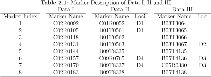
2.4.1 Dataset . . . 48
2.5 Results . . . 50
2.5.1 Unlinked loci . . . 50
2.5.2 D1-D4 multi-locus effects . . . 50
2.5.3 D2-D3 multi-locus effects . . . 51
2.6 Discussion . . . 51
2.7 Acknowledgments . . . 54
List of References 55 3 MDR-Phenomics 61 3.1 Abstract . . . 62
3.2 Introduction . . . 63
3.3 MATERIALS AND METHODS . . . 66
3.3.1 MDR-Phenomics . . . 66
3.3.2 Analysis of Power and Type I error . . . 70
3.3.3 Analysis of multi-locus effect . . . 71
3.3.4 Analysis of Autism . . . 71
3.4 Results . . . 72
3.4.1 Power and Type I Error of 1-locus model . . . 72
3.4.2 Analysis of multi-locus effect . . . 74
3.4.3 Analysis of Autism Data . . . 75
3.5 Discussion . . . 76
3.6 Acknowledgments . . . 80
List of References 81 4 PHD Method 95 4.1 Abstract . . . 96
4.2 Introduction . . . 97
4.3 Materials and methods . . . 99
4.3.1 Association test and sample classification . . . 99
4.3.2 Existence test of ID . . . 101
4.3.3 Definition of ID . . . 102
4.3.4 Data simulation . . . 105
4.3.5 Analysis . . . 106
4.4 Results . . . 107
4.4.1 Power and type I error: test of existent ID . . . 107
4.4.2 Efficient analysis . . . 107
4.5 Discussion . . . 109
List of References 115
5 Discussion 128
5.1 Introduction . . . 129
5.2 Multifactor Dimensional Reduction and Permutation Test . . . 129
5.3 Measuring Genetic Heterogeneity . . . 132
5.4 Dissecting Heterogeneous Phenotype . . . 134
5.5 Future Direction . . . 135
List of Tables
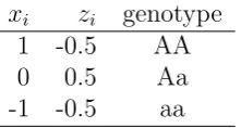
1.1 Definition of Dummy Variable for Genotype at Interaction Model . . 41
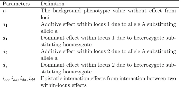
1.2 Definition of Parameters at Interaction Model . . . 42
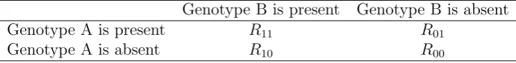
1.3 Relative Risk of two-locus model . . . 43
2.1 Marker Description of Data I, II and III . . . 56
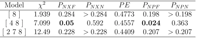
2.2 non-crossvalidation analysis of Data I . . . 57
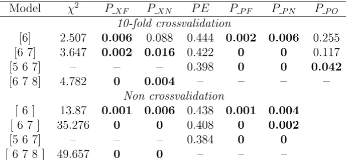
2.3 Analysis of Data II . . . 58
2.4 Analysis of Data III . . . 59
2.5 D2-D3 effect of Data . . . 60
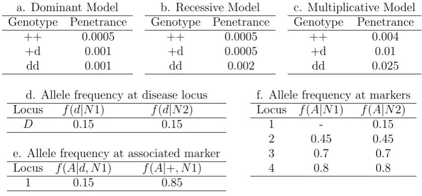
3.1 Disease Model and allele frequency . . . 85
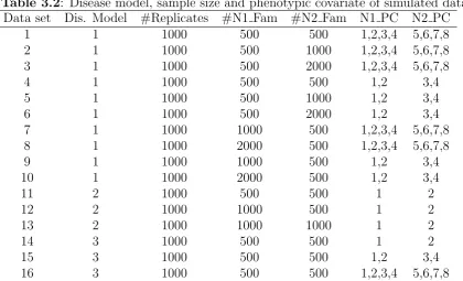
3.2 Disease model, sample size and phenotypic covariate of simulated data 86 3.3 Genes and markers in Autism data . . . 87
3.4 Type I error and Power . . . 88
3.5 a. Power of multi-locus effects . . . 90
3.6 LD Analysis of Autism Data . . . 92
3.7 locus model of Autism data . . . 93
4.1 Genotype penetrance under different inheritance . . . 118
4.2 Allelic frequencies in group N1 and N2 . . . 119
4.3 Inheritance, sample size and categorical phenotype . . . 120
4.4 test of existent of ID for categorical phenotype . . . 121
4.5 test of existent ID for continuous phenotype . . . 122
4.6 efficient analysis of categorical ID . . . 123
List of Figures
3.1 MDR-Phenomics Algorithm . . . 94
Chapter 1
1.1
Overview of Disease Gene Mapping
After complete sequence of human genome, more researches are focused on studies
of genetic causes. Determination of genetic causes facilitates the development of new
therapies and interventions. Human genetic diseases are generally classified into two
categories, simple disease (or Mendelian disorder) caused by a single gene mutation
and complex disease caused by the interplay of more than one genetic variant.
Com-plex disease can be further stratified into oligogenic and polygenic disorders, where
a few (oligogenic) and many (polygenic) genetic variants are involved respectively
(Singleton, 2003). However, this classification is not absolute, since complex disease
can have the Mendelian subforms too.
Linkage analysis has been the primary method for mapping Mendelian disorders
(Baron, 1999; Jorde, 2000). A classical successful example of linkage analysis is the
identification of cystic fibrosis gene in 1989 (Kerem et al., 1989; Riordan et al., 1989).
Following linkage analysis, a study of association based on linkage disequilibrium
(LD) is generally taken for fine mapping gene localization. Linkage and association
studies can locate a gene responsible for a disease when little or no information
is known about the molecular basis of the disease. Successful genetic mapping of
simple Mendelian disorders arouses interests and efforts in mapping complex
(non-mendalian) disorders caused by multiple genes and environmental influences. Linkage
analysis is the main method to study Mendlian disorders, but it is inefficient to search
for common variatns with modest effects underlying complex disease. Association
studies are the main method for complex disease gene mapping. However, linkage
analysis is not completely abandoned for complex disease and it still plays some
roles, especially in mapping Mendelian subforms of complex disease. Identification of
genes underlying Mendelian subforms by linkage analysis could shed light on other,
1.2
Genetic basis of mapping
A position on the chromosome is called a locus. A locus with varied DNA sequences
in the population, i.e. polymorphism, can be used as a genetic marker for analysis.
A marker allele is one of the variant forms of a DNA sequence at a locus. The
first type of polymorphic markers were restriction fragment length polymorphisms
(RFLP) (Botstein et al., 1980). An allele of a RFLP marker can be: 1) status of
absent or present endonuclease restriction site; or 2) varied number of tandem repeat
(VNTR) (Nakamura et al., 1987); or 3) varied number of simple sequence repeat (SSR)
(Jacob et al., 1991). Minisatellite sequence is the core unit of tandem repeat from
11 to 60 base pairs (Jeffreys et al., 1985). A simple sequence repeat is a repetitive
series of di-, tri- or tetra-nucleotide referred to as ”microsatellite” (Litt and Luty,
1989) or ”Short Tandem Repeat” (Edwards et al., 1991). Both kinds of repeats are
flanked by conserved endonuclease restriction sites. With development of Polymerase
Chain Reaction (PCR) technology in 1986 (Mullis et al., 1986), an economical marker
called Random Amplified Polymorphic DNA (RAPD) can be easily generated by
arbitrarily using short length of oligonucleotide PCR primers (Williams et al., 1990).
The third type of marker is the single nucleotide polymorphism (SNP). It refers to
a single nucleotide change, e.g., a nucleotide A, replacing one of the other three
nucleotides -C, G, or T. Generally, common SNPs have only two alleles and their
minor allele frequencies are at least 1%. Compared to other kinds of markers, SNPs
have the following advantages. First, SNPs are stable and abundant. They account
for approximate 90% genetic variation in human genome (Collins et al., 1998). There
are over 5,000,000 SNPs that have been well-curated and validated in public database,
dbSNP (http://www.ncbi.nlm.nih.gov/SNP/). Second, SNPs are easy and efficient
to detect. Hundreds of thousands of SNPs can be genotyped with low cost in only a
couple of days by high-throughput technologies (e.g. Affymetrix SNPchip, Illumina
and Taqman SNP platform) (Taillon-Miller et al., 1999; Wang et al., 1998). Third, by
any potential associations with disease (Kruglyak, 1999). These advantages make
SNPs one of the most popular markers in disease mapping today.
Penetrance describes the probability that a phenotype is expressed for a particular
genotype. In disease mapping, penetrance generally measures dichotomous status of
disorder (affected or not). A quantitative measure of phenotypic trait is expressivity,
which refers to what degree of a phenotype is expressed. Expressivity depends on
penetrance. It is impossible to measure expressivity if a genotype is not expressed
as a phenotype. Generally, for a marker with two alleles, A and a, if allele A is
dominant, the penetrance of genotype AA and Aa is similar. If allele A is recessive,
the penetrance of genotype AA is larger than that of genotype Aa and aa. Under
additive inheritance, the penetrance of genotype Aa is approximately the average of
penetrance of genotype AA and aa.
To save time and resources looking for genetic causes of non-genetic disease, it
is essential to assess the genetic component within a disease before gene mapping.
This may be accomplished by tracking the pattern of inheritance by analysis of
pen-etrance and expressivity. However, only Mendelian diseases exhibit a clear pattern
of inheritance, which is seldom apparent for complex disease. To evaluate the
ge-netic component especially of complex diseases, twin studies of concordance rates of
a phenotype in monozygotic and di-zygotic twins are widely used. If there is genetic
component, it is expected that monozygotic twins will carry 100% concordance rate
of a disease, while dizygotic twins will carry only 50%.
1.3
Linkage Analysis
Linkage analysis tests for coinheritance of chromosomal regions with a trait by
ex-tracting inheritance information (Kruglyak et al., 1996). For a disease locus D and
a gene marker M, co-segregation of allele is tested within a family to determine if
basis of linkage analysis is recombination or crossing-over that reflects physical
dis-tance between locus D and marker M. Recombination refers to chromosome arms
exchanging a segment of DNA sequence in meiosis where gametes (eggs and sperm)
are produced and two copies of each chromosome pair become physically close. If
recombination is random, the closer the locus D and M are on a chromosome, the
less frequently they will recombine. The recombination fraction, ranging from 0 to
0.5, increases monotonically as the distance of locus D and M increases. In principle,
locus D and M are linked if the recombination fraction between them significantly
deviates from 0.5. Linkage analysis can be classified into two categories, parametric
(or model-based) and non-parametric linkage analysis.
Parametric linkage methods directly test whether an observed recombination
frac-tion between two loci is significantly deviates from 0.5 (Ott, 1999; Terwilliger and Ott,
1994). The logarithm of odds (LOD) score is one of the most widely used approaches
for parametric linkage analysis (Morton, 1955). It is defined as below:
Z(θ) = log(L(θ)/L(0.5))
θ: Recombination fraction
Z(θ) : LOD score
L(θ) : Likelihood function with givenθ L(0.5) : Likelihood function with θ = 0.5
The parametric likelihood ratio test requires specification of disease parameters
in-cluding recombination fraction, marker allele frequencies, penentrance and disease
allele frequency. The drawback of the parametric linkage method is that the genetic
model must be known (Kruglyak et al., 1996) and the analysis can be highly sensitive
to misspecification of the linkage model (Clerget-Darpoux et al., 1986). For complex
diseases, the parameters above are generally unknown and mode of inheritance is
unclear, which restricts application of linkage analysis. The incorrect specification of
the mode of inheritance may lead to loss of power. However, some evidence shows
robust model for detecting linkage in complex diseases based on simulation studies,
in spite of the fact that the model is not entirely correct(Abreu et al., 1999; Durner
et al., 1999; Greenberg et al., 1998).
When inheritance patterns are not clear, non-parametric (or model-free) linkage
methods are more appropriate. Affected sib-pair (ASP) methods have been developed
to detect linkage by testing probabilities of Identical by Descent (IBD) sharing in
affected sib-pairs. IBD means that the same copy of an allele is inherited from a
common ancestor. For affected sib-pairs, the expected probabilities for sharing 0, 1
and 2 marker alleles IBD are 0.25, 0.5 and 0.25 respectively. Excess IBD sharing
indicates the analyzed marker is close to a susceptibility locus, which can be tested
by statistical methods like two-allele, mean and goodness-of-fit tests (Blackwelder
and Elston, 1985). When IBD is not known, identity by state (IBS) sharing among
affected members of the pedigree can be analyzed as a complement. The extent
of IBS sharing is compared with the Mendelian expectation under the hypothesis
of no linkage. Such a method is called affected-pedigree-member method (APM)
(Weeks and Harby, 1995; Weeks and Lange, 1988, 1992). APM sidesteps tracing the
inheritance pattern while focuses on the IBS sharing. A more general method called
non-parametric linkage (NPL) is proposed by Kruglyak to conduct multipoint linkage
analysis (Kruglyak et al., 1996).
Parametric and non-parametric methods have their advantages and disadvantages.
If the pattern of inheritance is known, parametric linkage methods often have larger
power than non-parametric methods (Goldin and Weeks, 1993), because the
recom-bination fraction between a disease susceptibility locus and a nearby marker from
non-parametric linkage tends to be an overestimate (Schork et al., 1993). However,
non-parametric methosd have unbeatable advantages for analysis of complex disease
with unclear inheritance.
When the molecular basis of the disease is unknown, a genome-wide linkage
2004b). Individuals within a pedigree generally have recent common ancestors and
recombination events do not occur often. Therefore, large regions of the genome are
shared and inherited between individuals within a pedigree. Most genome-wide
link-age analysis scans genome with fewer than 500 microsatellite markers spaced at 10Mb
distance. With advances of high throughput technology, a SNP array was recently
proposed for genome-wide linkage analysis for its efficiency and precision (Sellick
et al., 2004). Because of insufficient recombination events, resolution for gene
map-ping is generally low and large pedigrees are often required for genome-wide linkage
analysis.For fine mapping, analysis of candidate genes following genome-wide linkage
study is often taken.
Genome-wide linkage analysis scans markers across genome sequentially, and the
multiple testing problem involving point-wise and genome-wise significance level has
to been addressed. The point-wise (or element-wise) significance level refers to the
threshold for a single test of linkage to be significant, while the genome-wise (or
experiment-wise) significance level refers to the threshold for any linkage across the
genome to be significant (Lander and Kruglyak, 1995). A traditional approach for
multiple testing is the Bonferroni correction. For example, given 400 markers in
analysis of genome-wide linkage, a point-wise significance level of α0 = 0.00013 will correspond to a genome-wide significance level ofα∗= 1−(1−α0)400 = 0.05 by the
Bonferroni correction. However, the Bonferroni correction does not consider whether
markers are correlated with nearby markers. A better solution for genome-wide
signif-icance level can be defined as (Lander and Kruglyak, 1995): α∗= 1−e−(C+2×G×X)×α0,
where
α∗: genome-wide significance level
α0 : point-wise significance level
C : number of chromosomes
G: the size of the gonome in Morgans (M)
Therefore, to get at a genome-wide significance level of 0.05, the point-wise
signifi-cance level should be α0 = 5×10⁻⁵ which corresponds to a LOD score of 3.3. It was
also pointed out that LOD score of 3 is equivalent to p-value of 10−4, but not a p-value
of 10−3 as is often mistakenly assumed. Two additional important point-wise signif-icance levels include: 1) a point-wise p-value of 1.7×10⁻³ corresponding to a LOD score of 1.9 for suggestive linkage, and 2) a point-wise p-value of 0.05 corresponding
to a LOD score of 0.59 for nominal evidence of linkage. For a non-parametric sib-pair
study, the LOD scores for point-wise significance level to declare nominal, suggestive
and significant linkage were given as 2.2, 3.6 and 5.4. The derivation of the
genome-wide significance levels above is based on the assumptions of an infinitely dense set of
markers and full marker information content. These assumptions may not be true in
practice. If assumptions are not met, permutation testing is recommended (Sawcer
et al., 1997). Permutation methods generate a large number of permuted data sets
simulated under the null hypothesis of no linkage in the genome. The genome-wide
p-value is the percentage of LOD scores from simulated data exceeding the observed
LOD score.
1.4
Association study
A disease-marker association can be explained by two genetic mechanisms: pure
association and linkage disequilibrium (LD) (Baron, 2001). A maker allele with the
pure association increases disease risk directly, while LD indicates that a marker is
likely close to a disease locus. LD describes allele frequencies at the two loci that have
not reached equilibrium in the population and it measures the dependence of alleles
at different loci. LD is affected by recombination between two loci. For unlinked loci,
the LD will decrease dramatically over generations. Therefore, LD between two loci
1.4.1
Measure of Linkage Disequilibrium
The concept of LD was proposed in the early twentieth century (Jennings, 1916) and
the first common measure of LD, D, was proposed in 1964 (Lewontin, 1964). Given a diallelic loci, A and B, the D is calculated as p11−p1 ×q1, where p11, p1 and q1
are the frequencies of genotype A1B1, alleleA1 and allele B1 respectively. Under the
null hypothesis of no LD, the D is expected to be zero. The model that describes D
dependent on recombination fraction and time is (Jorde, 2000): Dt =D0×(1−θ)t,
where Dt is the D measured at the time in generations (t) since the origin of a
new disease-causing mutation and D0 is the D measured at the origin of mutation.
Thus, D can provide a simple estimation of the recombination fraction and can be used to infer the time since the origin of mutation. Other than the D, several other measurements were developed and applied in different cases. The standardizedD(D0) calculated asD/Dmax was developed to control allele frequencies, where the Dmax is given as min(p1q2, p2q1) and thep2 and q2 are values of 1−p1 and 1−p2 respectively.
The third measurement of LD is the correlation coefficient labeled as R or ∆, whose value is calculated as D divided by √p1 ×p2×q1×q2 (Hill and Robertson, 1968).
The fourth scale of LD is a two-locus disequilibrium statistic,δ, given byD/(q1×p22)
(Bengtsson and Thomson, 1981) where the p22 is the frequency of genotype A2B2.
To measure LD among multiloci, a scale parameter,λ, as extension of theδ statistic was proposed (Devlin and Risch, 1995)
LD in the human genome varies widely and differs markedly across genomic regions
and populations. In European populations, the LD extends around 10-30 kb, while it
extends much less in African populations (Ardlie et al., 2002). The different extent of
LD in the different populations suggests that a fine-scale mapping can be performed
in the African population, since the smaller extent the of LD , the better the mapping
1.4.2
Statistical tests of Linkage Disequilibrium
Association studies generally fall into two categories: population-based case-control
studies and family-based studies. The traditional family-based studies can be further
classified as discordant sibling tests and transmission disequilibrium tests with their
derivatives. For the population-based studies, a sample of unrelated affected
indi-viduals and unaffected controls are independently collected. Statistical methods, e.g.
goodness-of-fit test and likelihood ratio test, are applied to detect whether the
fre-quency of an allele or a genotype is associated with the affection status (Terwilliger,
1995). To analyze family data, an affected individual can be selected as a case and a
non-affected family member can be selected as a control for analysis. More powerful
population-based methods were developed to make use of all of the cases in a family
by considering the correlations among the related cases (Browning et al., 2005; Risch
and Teng, 1998; Teng and Risch, 1999).
Sometimes, it may be very hard to interpret a significant association based on the
population-based method, because the unrelated cases and controls may experience
different external factors, which are often called confounding factors in the
statisti-cal theory. A common confounding factor is population structure (i.e. admixture,
heterogeneity, or stratification in a population) that is reflected due to the different
background of the allelic frequencies in different populations. Generally, random
mat-ing is not allowed across different ethnic subgroups. It is possible that any disease
with a high frequency of incidence in one subgroup may be positively associated with
any allele more frequently within that group than other groups (Marchini J, 2004),
which can cause a spurious association. Several empirical examples showed evidence
of spurious association from the population structure (Knowler et al., 1988; Lander
and Schork, 1994; Reich et al., 1999). A classical example is the association study of
Gm haplotype with type 2 or non-insulin-dependent-diabetes mellitus (NIDDM) in
a sample of 4,920 native Americans of the Pima and Papago tribes (Knowler et al.,
tribes.
Since relatives within a family are more likely to share common confounding
fac-tors than unrelated individuals in a population, it could be more efficient to control
the population structure by using the family-based method. An early example is
haplotype relative risk (HRR) method (Falk and Rubinstein, 1987). The HRR tests
for association by defining the haplotype (or allele) transmitted from a parent to an
affected offspring as a ”case” and the untransmitted parental haplotype (or allele) as
a ”control”. In this way, the ”control” is clearly from the same population as the
”case”, which reduces effects of stratification. To get the ”control”, the HRR requires
markers of both the parents and their child to be genotyped. Let ”A” denote the the
allele of interest and ”a” to be the other one. If the affected child has genotype ”A/a”
and his parents have genotypes ”A/a” and ”a/a”, the HRR constructs a ”control”
with the genotype ”a/a”, since they are not transmitted from the parents to the
af-fected child. Then, the frequency of cases carrying ”A” allele (i.e, the number of cases
with genotype including ”A”) can be compared to the frequency of controls carrying
it under the null hypothesis that the frequencies are equal. Tests are conducted by
the traditional case-control methods with Pearson’s chi-square contingency statistic
or odds ratio. For a rare disease, the odds ratio approximates the relative risk and its
expected value is 1.0 under the null hypothesis of random transmission. Rejection of
the random transmission of a haplotype indicates the existence of association.
Con-sidering the principle of HRR, despite the fact that the ”controls” are constructed
from non-transmitted parental alleles, the test assumes that both of the ”controls”
and ”cases” are randomly and independently drawn from their population. The
inde-pendence assumption will be violated if recombination occurs. Therefore, the HRR
tests association under the the existence of linkage. For a rare disease, the HRR
applies the odds ratio to estimate the relative risk and Knapp proved that the
rela-tive risk for the susceptibility locus may be underestimated if there is recombination
The transmission-disequilibrium test (TDT), a modified form of HRR, was
pro-posed in 1993 (Spielman et al., 1993). In contrast to the HRR that tests for an
association with the existence of linkage, the TDT tests for linkage in the presence
of association or association in the presence of linkage. The TDT and its derivatives
have become the popular methods to evaluate the linkage and association of a marker
and screen a genome for susceptibility loci (Schwab SG, 2000; Sun et al., 1999). The
TDT analyzes triad families, i.e. an affected offspring and his/her parents. A major
difference between TDT and HRR is that parents for TDT must be heterozygous to
be informative.
Let ”A” to be the allele of interest and ”a” to be all of the other alleles at a locus.
For the heterozygous parents, their genotypes are ”A/a”. Let ”nA” to be the number of times that the heterozygous ”A/a” parents transmit ”A” to the affected child and
”na” to be the number of times that the heterozygous ”A/a” parents transmit ”a”
to the affected child. Given the heterozygous ”A/a” parents, transmission of ”A” (or
”a”) indicates non-transmission of ”a” (or ”A”), so the transmissions of ”A” and ”a”
is perfectly negatively correlated. To control the correlation between allele ”A” and
”a”, the TDT applies a McNemar’s chi-square statistic to test random transmission
of ”A” and ”a”. Under the null hypothesis of random transmission, ”nA” falls in a
binomial distribution, bin(n, p), where n =nA+na and p= 0.5. The TDT statistic
by the McNemar test is calculated as (nA−na)2/(nA+na) (Spielman and Ewens,
1996; Spielman et al., 1993). The distribution of the TDT approximates a chi-square
distribution with degree of freedom equal to 1. The random transmission can be
generated by either non-linkage or non-association. However, complete understanding
and interpretation of the test is not easy. To understand the test, let us consider
linkage without association first. Because the linkage phase is unknown in a sample
of triad families, two linkage phases exist with equal probability. For example, suppose
the disease genotype is D/N and the marker genotype is A/a. The two linkage phases
of a marker allele. Second, association without linkage causes the two linkage phases
to occur with unequal chances. Since linkage does not exist, recombination events
will make segregation of alleles to the affected child occur randomly, and again the
TDT will give non-significant results due to the random transmission of the candidate
alleles. More specifically, the null hypothesis of the TDT test can be expressed as
the equation: δ ×(1−2×θ) = 0, where δ = 0 means absence of an association and θ = 0.5 means absence of a linkage. Rejection of the null hypothesis indicates that both linkage and association exist. An example of the TDT is the test for two
active forms of Catechol-O-methyl transferase (COMT). The TDT confirmed that
the high-activity form was preferentially transmitted in schizophrenia (Li T, 1996).
The TDT eliminates stratification effects, but a disadvantage is that it uses only
heterozygous parents. When there is no stratification, it will be less powerful than the
HRR, which uses both homozygous and heterozygous parents (Schaid, 1998). When
there is stratification, the HRR (or similar tests such as AFBAC (Thomson, 1995) is
more likely to yield a false positive result (Spielman and Ewens, 1996).
Numerous variants of the TDT have been devised, including the extensions for
multiallelic markers (Sham and Curtis, 1995), multiple marker loci (Wilson, 1997),
quantitative trait loci (Allison, 1997; Xiong et al., 1998), extended pedigrees (George
et al., 1999), families in which only one parent (Sun et al., 1999; Weinberg, 1999)
or only siblings are available (Martin et al., 2003), sib-TDT (Allison et al., 1999;
Spielman and Ewens, 1998; Teng and Risch, 1999), and the Pedigree Disequilibrium
Test (Martin et al., 2000). The sib-TDT is especially useful for diseases of late
adulthood, in which multiple generations may not be available for the study. However,
the sib-TDT may be less powerful than the traditional TDT (Schaid, 1998). Another
variant of the sib-TDT examines allele-sharing patterns in sibs who are discordant
for a trait (Boehnke and Langefeld, 1998).
The Pedigree Disequilibrium Test (PDT)(Martin et al., 2000) is often cited and
was integrated in the novel methods discussed in this paper. In contrast to the TDT,
and discordant sib-pairs. Since the nuclear families and the discordant sib-pairs (DSP)
from the same extended pedigree are related, the PDT treats extended pedigree as
independent units and measures LD in a pedigree by a statistic, D. Considering a marker locus with two alleles, the D statistic of a pedigree is calculated as follows:
D= n 1
T+nS
nT
∑
j=1
XT j + nS
∑
j=1
XSj
nT : the number of triads nS : the number of DSPs
XT j = (# M1 transmitted) - (# M1 not transmitted) in j - th triad family
XSj = (#M1 in affected sib) - (# M1 in unaffected sib) inj - th DSP
If N is the total number of unrelated pedigrees in the sample and Di is the random
variable for the ith pedigree, then under the null hypothesis of no linkage disequilib-rium, we can get:
E(
N
∑
i=1
Di) = 0
V ar(
N
∑
i=1
Di) = N
∑
i=1
V ar(Di) = E( N
∑
i=1
D2i)
T =
N
∑
i=1
Di/ N ∑ i=1 D2 i (1.1)
The T statistic in the equation 1.1 for a large sample will have asymptotically standard
normal distribution with a mean of 0 and a variance of 1.
The power and efficiency of association tests depend on many factors, including the
methods used, the sample size, the mode of inheritance, the patterns of recombination
and genetic heterogeneity as well. Genetic heterogeneity, which is common in complex
diseases, may cause the power decrease dramatically (Xiong and Guo, 1998). All of
these factors can result in no increase of the power of an association method though
1.4.3
Genome-wide association analysis and statistical
sig-nificance
In the past decade, hypothesis-driven candidate gene association studies have become
popular, but these are usually limited to a few dozen of genes. With the development
of high-throughput genotyping technology, it is now possible to apply the genome-wide
association studies for mapping diseases. Genome-wide association studies require a
much more dense set of markers than the genome-wide linkage studies do. However,
it is inefficient to genotype all of the existing common polymorphisms. To attain fine
resolution with cost efficiency, generally only the tag SNPs or markers with linkage
equilibrium are genotyped for genome-wide association studies. Use of tag SNPs is
possible for genome-wide association studies, since the existence of the recombination
hotspots makes the pattern of LD in the human genome block-like (Ardlie et al.,
2002; Gabriel et al., 2002). Therefore, a minimum number of SNPs in a block used
as the tag SNPs can be selected to represent the genetic variation in that block
without genotyping all of the SNPs. The association mapping, e.g. the International
HapMap Project (Consortium, 2003), now allows selection of the tag SNPs on the
basis of publicly available data.
A wide association study generally requires more markers than a
genome-wide linkage study, and it is more challenging for the genome-genome-wide association study to
adjust for multiple tests. For genome-wide linkage analysis, the multiple tests are
effi-ciently controlled and the LOD score of 3.3 generally corresponds to the
experiment-wise type I error of 0.05 as discussed above. However, there is no consensus on the
standard of adjusting for the multiple tests in the genome-wide association studies
(Elston, 1997; Kruglyak, 1997; Morton, 1998). The Bonferroni method can be applied
for the control of multiple tests, but it can cause overcorrection easily and has the
risk of failing to detect the true association. To prevent the overcorrection, many
advanced methods were developed. It was proposed to estimate the probability
tested marker can be obtained directly (Schork, 2002). However, estimation of the
probability distribution in a population is genome-region specific. Another common
method is called empirical Bayes (EB) or semi-Bayes adjustments (Greenland, 2000;
Greenland and Robins, 1991). The basic idea of the EB adjustments is that the
ob-served statistic for an individual test has larger variation than the true one, although
the statistic may be unbiased. The large variation will cause increase of the type I
error. The EB attempts to estimate an inflated variation from the observed data and
uses this estimation to adjust the observed statistic. The process of this adjustment
is called shrinkage, since the adjusted individual statistic generally has a decreased
variation. The advantage of the EB adjustments is that a prior probability can be
integrated. For example, a genomic region known to contain a causative variant will
be assigned a high prior probability for the EB adjustments.
1.5
Characteristics of Complex Disease Gene
Map-ping
Successful identification of genetic variants by linkage and association studies depends
on the type of genetic variants underlying a disorder. We often consider two types of
variants, the rare and the common variants. Variants with large or early deleterious
effects are mostly rare (Pritchard, 2001). Rare variants are generally young and
relatively geographically localized. It is difficult to identify rare variants in a small
sample. In contrast, common variants are generally old and geographically dispersed.
It is relatively easy and cheap to identify the common variants. Linkage analysis is
generally more powerful than association analysis for identifying the rare, high-risk
disease alleles (Weiss and Clark, 2002). However, fine resolution of mapping a rare
allele with large effect through the linkage analysis is feasible only with the availability
of sufficient recombination events, which requires large pedigrees (Boehnke, 1994).
quite common in a population for most cases, ie. the Common Disease/Common
Variant (CD/CV) hypothesis (Chakravarti, 1999; Lander, 1996). Each of the
com-mon variants in a complex disease only has a small or modest effect on the disease
phenotype, while multiple common variants can act additively or have multiplicative
interaction (epistatic effect). Linkage mapping analysis generally does not have
suf-ficient power to identify common variants with a small effect, because conventional
linkage methods are generally based on the assumption that the genotyped markers
work independently and a single gene has a large main effect on the disease (Buhler
et al., 1997; Cox et al., 1999; Hoh and Ott, 2000; Lucek et al., 1998). Because of
this, linkage mapping is the preferred method for mapping genes having
moderate-to-large effect on Mendelian disorder. In contrast, most of the association studies
have the ability to analyze a haplotype of multiple markers or an interaction between
the markers (e.g. regression analysis). There is a general consensus that association
analysis should be more powerful for detection of the common disease alleles with
modest disease risks than the linkage analysis (Risch and Merikangas, 1996). In
ad-dition, there are two other reasons that may limit the use of the linkage methods and
support the association studies. First, a complex disease generally does not have a
clear inheritance pattern. The linkage analysis is often based on a clear inheritance
(e.g. calculation of LOD). In contrast, most association studies generally do not
re-quire clear inheritance. Second, linkage studies, especially the traditional parametric
methods, cost a lot for the collection of a large pedigree. Instead, the association
analysis especially the population-based case-control studies can be economical and
easier.
However, linkage analysis is still a common method applied in mapping complex
diseases based on the assumption that there are Mendalian subforms of complex
dis-ease with genes having large effects. Successful examples include Alzheimer’s disdis-ease
(beta-amyloid precursor protein and presenilin-1 and -2), breast cancer (BRCA-1 and
-2), colon cancer (familial adenomatous polyposis and hereditary non-polyposis
glaucoma (Baron, 2001). These successes provide useful information of the common
forms of complex diseases and can give us a guidance for more complex association
studies. Such a successful guidance is the mapping of a complex disease, open-angle
glaucoma. Its association analysis is focused on the region which is detected by the
linkage analysis of its Mendalian subform, juvenile open-angle glaucoma (Stone et al.,
1997). However, Mendelian subforms of the complex diseases are generally rare and
hard to identify. Therefore, linkage analysis of incorrect Mendelian subforms may
easily miss the true causative genes.
Although linkage mapping may not be the most appropriate method for complex
diseases, it does not mean that the linkage methods can not detect genes with modest
effect underlying a complex disease (Scott et al., 1997). Such an example is APOE
successfully identified as a susceptible gene of the late onset of Alzheimer’s disease
by using microsatellite marks in a linkage mapping. Another example is HLA, which
was identified by multipoint linkage analysis of affected sibpairs in mapping type I
diabetes (Concannon et al., 1998). However, it must be noticed that a large sample
size is generally required for a linkage analysis to get adequate power in discovering
genes with small effects. Therefore, although the linkage analysis may continue to
play some roles, association studies are the major and superior strategies for mapping
complex diseases (Risch, 2000).
Multiple characteristics of complex diseases, including heterogeneity, complex
epistatic effects and the curse of dimensionality due to interaction in high-order
di-mensionality, mean that pursuing more advanced methods is always needed. For most
of the complex disease mapping, the study designs are often observational and many
unknown factors can not be controlled. Therefore, two statistical issues, bias and
confounding, may conflict mapping results. In general, mapping results are used to
provide guidance for the further research on gene function. Mapping strategies and
1.5.1
Mapping strategies
Since there is not a method which is sufficient or optimal for the mapping of the
com-plex diseases, multiple solutions are often required. It is suggested that a combination
of the linkage and association analysis, including the follow-up of candidate
chromo-somal regions, may be more efficient than either one method alone (Baron, 2001). A
direct and cost effective strategy is candidate gene based studies. The identified and
genotyped SNPs within the candidate genes are analyzed by the linkage and
associa-tion methods (Cambien et al., 1999; Cargill et al., 1999). In contrast to the candidate
gene strategy, three popular genome-wide mapping strategies for complex diseases
are often applied. The first strategy conducts genome-wide linkage analysis by using
anonymous DNA polymorphisms, and is followed by candidate association studies to
analyze more genotyped SNPs around the markers with linkage signal for fine mapping
(Botstein and Risch, 2003). The second strategy applies the indirect genome-wide
association with anonymous SNPs (or ”tagSNPs”) followed by the candidate
associ-ation studies (Concannon et al., 1998). The third strategy is direct genome-wide LD
mapping that uses tens or hundreds of thousands of candidate-SNPs (coding or
pro-moter variants with potential functional significance) to infer the causative variants
(Collins et al., 1997; Risch and Merikangas, 1996). Indirect genome-wide association
studies may be more efficient and powerful than the classical direct whole-genome
association studies, since directly testing all of the common functional variants may
lose important markers in the non-coding regions.
Genome-wide association studies require many more SNPs than genome-wide
link-age studies. In contrast to select the functional SNPs in coding regions in the direct
genome-wide association studies, the indirect genome-wide association studies use
anonymous SNPs, which makes it more challenging and strategic. To reduce cost and
improve efficiency in selecting and genotyping the anonymous SNPs, developing an
association map characterized with patterns of LD across the genome is necessary.
Based on the CD/CV hypothesis, the HapMap project was initiated by both of the
of common SNPs, which can be used to direct the selection of markers for the
indi-rect genome-wide association study. The HapMap describes the common patterns of
human genetic variation by identifying the chromosomal regions (”blocks”) and the
tag SNPs along the human genome (Altshuler D, 2005; Consortium, 2003). Since the
variants in these regions often have strong LD, the possible number of haplotypes in
these regions will be greatly decreased. Based on this fundamental theory, it is not
necessary to genotype all of the SNPs in these regions for the association studies.
Instead, we only need to identify about 300,000 to 600,000 tag SNPs to capture the
genetic variations of 10 million common SNPs with a minor allele frequency (MAF) of
at least 5% across the entire human population. The detailed process is implemented
by genotyping tag SNPs in the affected and unaffected samples, and the patterns of
association between the tag SNPs and the disease markers are tested by the
popu-lation based case-control studies (e.g. classical chi-square) or family based studies
(e.g, Transmission Disequilibrium Test) (Hirschhorn and Daly, 2005). If a significant
association exists, researchers can identify the functional variants by focusing on the
regions with strong LD to tag SNPs (Concannon et al., 1998).
To prevent over-conservative results due to adjusting for the analysis of a large
number of markers in the candidate-gene method or the genome-wide studies,
some-times, a two-stage design is used for analysis. The two-stage design for genome-wide
studies was first proposed by Sobell et al. in 1993 (Sobell et al., 1993), where an
initial sample was tested for a dense set of markers, and then an independent sample
was tested only on a subset of the most ”significant” markers. The design has
re-cently been extended to the genome-wide scan with methods developed to optimize
the sample size and the significance levels at each stage to maximize the power and
constrain cost and the overall type I error (Lowe et al., 2004; Satagopan and Elston,
1.5.2
Heterogeneity
Population stratification is a kind of heterogeneity conflicting analysis of both Mendelian
and complex diseases, and it is generally generated from past historical events,
in-cluding admixture, genetic drift, multiple mutations, natural selection, etc. Genetic
heterogeneity, in which the same or similar phenotypes of a complex disorder is caused
by different susceptibility genes (Davies et al., 1994), complicates the analysis of
complex diseases. Many diseases such as diabetes, ischaemic heart disease, asthma,
schizophrenia, Alzheimer and many psychiatric diseases (e.g. autism) are shown to
be genetically heterogeneous. Generally, there are two types of genetic heterogeneity:
(1) allelic heterogeneity where a disorder phenotype is caused by different mutations
within a locus; and (2) locus heterogeneity where mutations at different loci can
pro-duce the same disease phenotype. Since genetic heterogeneity can conflict with both
linkage and linkage disequilibrium in a population, it is believed that the traditional
linkage and association studies work better in the genetic homogeneity (Baron, 2001;
Pritchard and Cox, 2002).
1.5.3
Epistatic effects: Gene-gene and Gene-environment
In-teraction
A gene-gene interaction occurs when the effect of one gene is modified or altered by
one or several other genes. Epistatic effect refers to a phenotype being enhanced
in the interaction, whereas hypostatic effect refers to a phenotype being suppressed.
Environmental factors can affect the expression of gene’s phenotypes in a similar way,
which is called gene-environment interaction. Both gene-gene and gene-environment
interactions are assumed to be common epistatic effects underlying complex diseases
(Carlson et al., 2004a).
Given an expressed phenotype, gene-gene interaction effects can be explained by
(locus 1 and locus 2) as an example, a synergistic epistatic effect refers to the
phe-nomenon, where the gene-gene interaction between the locus 1 and the locus 2 creates
an effect greater than the predicted effect for either locus acting alone, and an
an-tagonistic epistatic effect refers to the phenomenon, where the gene-gene interaction
creates an effect smaller than the predicted effect for either locus acting alone. When
there is no epistatic interaction, the effects from the locus 1 and the locus 2 are
addi-tive. The epistatic model from two diallelic loci with alleles denoted as A and a can
be explained mathematically by using a linear model. For a quantitative phenotype,
the mathematical model is described as (Cordell, 2002):
y=µ+a1x1 +d1z1+a2x2+d2z2+iaax1x2+iadx1z2+idaz1x2+iddz1z2 (1.2)
The y is a quantitative phenotype and the genotypes at the locus 1 and the locus 2 are represented by a dummy variable xi and zi respectively (Table 1.1). Coefficients
of the linear model 1.2 are defined in the table 1.2. When there is no epistatic effect,
the model 1.2 is simplified as the additive effect:
y=µ+a1x1 +d1z1+a2x2+d2z2 (1.3)
The complex linear model can be simplified further as:
yij =αi+βj +Iij (1.4)
In model 1.4, the quantitative yij refers to a phenotypic value with the genotypeiat
locus 1 and the genotypej at locus 2. Parameters ofαi andβj are the genetic effects with genotype iat locus 1 and the genotypej at locus 2 respectively. The parameter
Iij is the interaction effect between locus 1 and 2. An additive effect occurs when Iij
is zero.
genotypej at locus 2 can replace theyij to describe the additive model and the
mul-tiplicative model aspij =αi+βj andpij =αi×βj respectively (Cordell, 2002; Hodge,
1981; Risch, 1990). A more clear definition of the epistatic model for a dichotomous
disorder can be explored by using the relative risk. We can denote the relative risks
of genotype A and B at two loci in 2-by-2 contingency table (Table 1.3).
If there is no epistatic effect, we can get equal relative risk ratios (R11/R01 =
R10/R00) and relative risk differences (R11−R01 =R10−R00). A Synergistic effect
should have an increased relative risk ratio (R11/R01 > R10/R00) and a relative risk
difference (R11−R01 = R10−R00). In contrast, an antagonistic effect should have
a decreased relative risk ratio (R11/R01 < R10/R00) and a relative risk difference
(R11−R01 < R10−R00). Based on these results, we can test what exactly the epistatic
model is by testing the relative risk ratio or the relative risk difference by using
wald, likelihood ratio or score method (Kupper and Hogan, 1978). For rare complex
diseases, the odds ratio approximates the relative risk ratio and the logarithm of
the odds ratio transforms the multiplicative scales to the linear scale, where a logistic
regression model can be applied in the test. Therefore, the multiplicative model of the
statistical interaction is sometimes called a log-linear or logistic model too (Breslow
and Storer, 1985).
1.5.4
High-order interaction and the curse of dimensionality
SupposeM common variants are involved in a complex disease. The gene-gene inter-action inM dimensionality is of high-order if theM is large (i.e. M >3). Accompa-nied with the high-order interactions, the curse of dimensionality may occur, where a
linear increase in dimension can cause an exponential increase in volume. Specifically,
for M di-allelic markers, the M-dimension corresponds to the volume of 3M, which
defines the exponential association between the volume and the dimension. Unless
if a large sample is not available. The second challenge is how to efficiently
iden-tify the high-order interactions, since the number of possible interactions for even
a relatively small set of candidate genes can be big. For example, 8 candidate loci
will have 28 possible two-factor interactions and 56 possible three-factor interactions.
Generally, forL(L > M) markers under analysis, the possible number of interactions is 2L−1. To correctly identify an interaction, it may necessary tests all of the
possi-ble 2L−1 interactions, which is laborious work and may produce a high demand of
computational load. Lastly, the problem of multiple test issue is unobviated in the
identification of a high-order interaction.
Comprehensive search in the high dimensional space for interactions generally
has poor power (Carlson et al., 2004a). To improve the power, the straight-forward
strategy is to reduce the number of loci, which can be implemented by selecting
only the candidate genes involved in the related biological pathway or picking the
independent loci without LD. However, to solve the multiple tests and the curse of
dimensionality, more advanced statistical methods are required.
In the past decades,many parametric and non-parametric methods have been
de-veloped to detect the high-order interactions. Logistic regression is a common method
used to model multiple genotyped loci simultaneously. Compared to parametric
meth-ods, non-parametric methods do not require specific assumptions of statistical and
genetic hypothesis, i.e. no estimation of parameters and no assumption of inheritance
are needed. Therefore, the non-parametric methods are better in searching for the
trends or patterns in the high-dimensional data sets (Moore and Ritchie, 2004). The
classification and regression trees (CART) (Sachidanandam et al., 2001) aims to build
classification tree by using binary predictors through three steps, growing the tree,
pruning the tree and selecting the optimal tree. Multivariate adaptive regression
splines (MARS) (Friedman, 1991) model the relationships between the responsible
variables and the predicator variables by partitioning the input space with high
with joint probability based on a probabilistic reasoning system. The set-association
method (Hoh and Ott, 2000) integrates the allelic association and the Hardy-Weinberg
disequilibrium (HWD) to identify the multiple-gene effects with the ability to
han-dle high dimensionality. The combinatorial partitioning method (CPM) works by
evaluating all of the possible partitions of marker loci and identifying the
multilo-cus genotypic partitions that predict quatitative trait variation based on a certain
optimality criteria (Venter et al., 2001). CPM successfully built the multi-locus
mod-els with interactions to explain and predict the variability in plasma triglyceride and
plasma plasminogen activator inhibitor 1 levels. Culverhouse et al. modified the CPM
to the restricted-partition method (RPM) (Reich et al., 1999) to heuristically restrict
the exhaustive search and reduce its computational load for evaluating interactions.
The multifactor dimensionality reduction (MDR) method (Ritchie et al., 2001)
was developed as an extension of the CPM to search high-order interaction for
di-chotomous disease. The MDR method has been widely applied recently. It divides
data into 10 equal parts. Within each 9/10 of the data, the MDR classifies the
multi-locus genotypes as either the ”high risk” or the ”low risk” depending on the ratio of
cases to controls. If the ratio is higher than 1.0, it is ”high risk”, otherwise, it is ”low
risk”. The best k-gene set is the one that maximizes the ratio in the pooled ”high
risk” group. The MDR uses the remaining 1/10 of the data to calculate the
predic-tion error and the consistency as statistics and applies permutapredic-tion test to get the
p-values. The MDR is shown successfully in finding gene-gene interactions in atrial
fibrillation and Type 2 diabetes. To tap the advantages by the association studies in
families, MDR-PDT (Martin ER, 2006) merged the MDR method with the
genotype-PDT (Martin et al., 2003) to test the association between disease and genotypes at a
locus or multiple loci jointly. The MDR-PDT allows the identification of single-locus
1.5.5
Bias and confounding
Statistical tests can not answer questions of biologically causativity of a variant or
pathway directly, instead, a significant linkage and/or association can only provide a
guidance to determine whether the finding is worthwhile pursuing further (Terwilliger
and Weiss, 1998). An accurate statistical test is important to give a correct guidance.
The accuracy is affected by confounding factors that are associated with both the
disease and the markers under study. The term of bias related to accuracy describes
the difference between the true parameter and the statistical estimator.
Association methods are often superior to linkage methods for mapping of complex
disease genes. However, association results are generally affected more by the
con-founding factors than linkage results. The bias due to concon-founding factors can cause
difficulty in the interpretation of the test results. A confounding factor in
population-based association studies is population structure, which can be prevented by checking
whether the genotype frequencies among cases and controls are in Hardy-Weinberg
equilibrium (Campbell and Rudan, 2002). Failure to follow Hardy-Weinberg
equilib-rium may suggest invalid results of the association study due to the possible large
bias. However, control of confounding factors may be never complete, since most of
the genetic studies are observational and it is not feasible to consider all of the possible
confounding factors. The strategies to control the confounding factors are generally
limited to only a small number of confounding factors. In many cases, in spite of
an individual factor contributing only a small confounding effect, the confounding
effect from multiple factors together can be substantial (Thompson, 1994), and it is
easy to miss one or several of these factors. To control for confounding factors, a
straight-forward strategy is trying to match individuals with as similar a background
1.6
Novel methods
Based on the special characteristics of the complex disease, we developed several
methods to improve the power of gene identification. To detect epistatic effects in the
high dimensionality, we extended MDR (EMDR) with alternative statistics, different
validation processes and permutation methods. By testing the known gene-gene
in-teractions in the simulated Genetic Analysis Workshop (GAW14) data with complex
genetic inheritance, we showed that EMDR works better than MDR with improved
computational load (Maher and Brock, 2005). To eliminate, or at least reduce the
effect of genetic heterogeneity, the MDR-Phenomics method was developed to
inte-grate a clinical phenotype for measuring the heterogeneity. Complicated simulation
tests showed that the MDR-Phenomics improves the power under all of the
simu-lated cases. Analysis of autism data by the MDR-Phenomics successfully identified
the interaction between the serotonin transporter gene [SLC6A4] and integrin beta
3 [ITGB3] on Chr 17. To address the problem of genetic and population
hetero-geneity, the algorithm of phenotypic homogeneous distinction (PHD) was developed
to get a phenotypic IDENTIFIER that is characteristic of homogeneous association.
The IDENTIFIER is applied back to recruit pedigree data for association studies.
Analysis of the simulated datasets under different heterogeneity shows that an
asso-ciation study integrated with an IDENTIFIER is more powerful than the traditional
List of References
Abreu PC, Greenberg DA, Hodge SE (1999). Direct power comparisons between
simple LOD scores and NPL scores for linkage analysis in complex diseases. Am J
Hum Genet 65(3):847–57.
Allison DB (1997). Transmission-disequilibrium tests for quantitative traits. Am
J Hum Genet 60(3):676–90.
Allison DB, Heo M, Kaplan N, Martin ER (1999). Sibling-based tests of linkage
and association for quantitative traits. Am J Hum Genet 64(6):1754–63.
Altshuler D Brooks LD CACFDMDP (2005). A haplotype map of the human
genome. Nature 437:1299–1320.
Ardlie KG, Kruglyak L, Seielstad M (2002). Patterns of linkage disequilibrium in
the human genome. Nat Rev Genet 3(4):299–309.
Baron M (1999). Candidate genes and behavioral traits–candidly! Arch Gen
Psychiatry 56(6):582–3.
Baron M (2001). The search for complex disease genes: fault by linkage or fault
by association? Mol Psychiatry 6(2):143–9.
Bengtsson BO, Thomson G (1981). Measuring the strength of associations between