ABSTRACT
CAPAN, MUGE. Optimal Patient-centered Response to Acute Physiological Deterioration of Hospitalized Patients. (Under the direction of Dr. Julie S. Ivy.)
In this research, we collaborate with the Division of Health Care Policy & Research, Department of Health Sciences Research, Mayo Clinic, Rochester. We seek to individualize the response to APD by using electronic medical records (EMRs). We use EWSs to capture the stochastic changes in a patient’s physiological condition during a stay in the general ward.
Optimal Patient-centered Response to Acute Physiological Deterioration of Hospitalized Patients
by Muge Capan
A dissertation submitted to the Graduate Faculty of North Carolina State University
in partial fulfillment of the requirements for the Degree of
Doctor of Philosophy
Industrial Engineering
Raleigh, North Carolina 2014
APPROVED BY:
_______________________________ ______________________________
Anita Vila-Parrish James R. Wilson
________________________________ ________________________________
DEDICATION
BIOGRAPHY
ACKNOWLEDGMENTS
I acknowledge with pleasure:
My advisor Dr. Julie Ivy, who introduced me to academic research, and who encouraged me to rise to challenges. She has always been a great teacher and a source of inspiration for me. I am honored to be a member of our academic family.
My mentor Dr. Jeanne Huddleston, who inspired me with her passion for enhancing health care science with Industrial and Systems Engineering tools. I am blessed for having a mentor who can translate medical science to engineering.
The other members of my dissertation committee, Dr. James Wilson, Dr. Peter Bloomfield, and Dr. Anita Vila-Parrish, for their feedback which helped improve this document.
Erinc Albey, Thomas Rohleder, and the Department of Health Sciences Research at the Division of Health Care Policy & Research at Mayo Clinic, with Todd Huschka, Joel Hickmann, Bruce Morlan, Matthew Johnson, Megan Reinalda, who introduced me to the Bedside Patient Rescue Project, and provided support to clean and analyze the data, which made this research possible. Thank you for all your time and effort.
My second family in the U.S., Irem Sengul Orgut, Gokce Akin Aras, Asli Ozen, Jivan Deglise-Favre-Hawkinson, Resulali Emre Orgut, and Korhan Aras, for sharing this adventure with me, and for making the journey worthwhile.
My dear friends scattered around the world, Deniz Dursun, Neslihan Ballik Erdogan, Burcu Ayoglu, Omur Sozer Senol, Linden Horvath, Selcuk Kuram, Klaus Angerer, Antje Herrmann, and Olga Willner, for making me feel at home on three different continents, and for sharing their experiences with me.
TABLE OF CONTENTS
LIST OF TABLES ... x
LIST OF FIGURES ... xii
LIST OF ABBREVIATIONS ... xiv
Chapter 1 Introduction ... 1
1.1 Problem Description ... 7
1.1.1 Challenge of Determining the Patients at Risk of Deterioration ... 7
1.1.2 Need for Dynamic Models ... 8
1.2 Research Question ... 10
1.3 Remaining Content of the Dissertation ... 11
Chapter 2 Literature Review ... 12
2.1 Markov Decision Process... 12
2.2MDP Applications in Health care ... 14
2.3 Semi-Markov Decision Process ... 16
2.4SMDP Applications ... 21
2.4.1 SMDP Applications in Machine Maintenance ... 21
2.4.2 SMDP Applications in Queuing ... 22
2.4.3 SMDP Applications in Finance ... 24
2.4.4 SMDP Applications in Health care ... 25
2.5 Contributions of this Dissertation ... 26
Chapter 3 Identification of Patient Populations Using Early Warning Scores ... 29
3.1Introduction ... 29
3.2Literature Review ... 30
3.3 Methodology ... 34
3.3.1 Model Formulation ... 35
3.3.2 Identification of Subpopulations ... 38
3.3.3 Statistical Tests ... 42
3.3.4 Results of the Statistical Tests ... 50
Chapter 4 A Decision Model to Inform and Personalize the Response to Acute and
Persistent Physiological Deterioration ... 61
4.1Introduction ... 61
4.2Background on Acute Medical Care ... 64
4.3Literature Review ... 67
4.3.1 Machine Maintenance Literature ... 68
4.3.2 Medical Decision Making Literature ... 69
4.4Model Formulation ... 71
4.4.1 Defining Model Components ... 73
4.4.2 Cost Structure ... 77
4.4.3 Optimal Value Function ... 87
4.4.4 Patient Classification ... 88
4.5Model Properties ... 89
4.5.1 Framework for the Structural Properties ... 90
4.5.3 Framework to Establish the Existence of Optimal Monotone Policies ... 93
4.6Case Study ... 100
4.6.1 Data and Model Parameterization ... 101
4.6.2 Numerical Results ... 104
4.6.3 Clinical Implications for Resuscitation Decisions ... 106
4.7 Conclusion ... 107
Chapter 5 A Modeling Approach to Capture Provider-specific Uncertainty to Inform Resuscitation Decisions ... 110
5.1Introduction ... 110
5.2Literature Review ... 113
5.2.1 Uncertainty in State Transition Probabilities ... 114
5.2.2 Uncertainty in Costs and Rewards ... 115
5.3Model Formulation ... 117
5.3.1 Generating Random Variables ... 117
5.3.2 Cluster Analysis ... 127
5.3.3 Linear Programming Formulation ... 135
5.4.1 Baseline Scenario Results ... 142
5.4.2 Modified Scenarios... 146
5.4.3 Linear Programming Results... 150
5.5Conclusion ... 155
Chapter 6 Conclusions ... 159
REFERENCES ... 164
APPENDICES ... 173
Appendix A. Existence of Inverses ... 174
Appendix B. Generalized Linear Model (GLM) with Repeated Measures ... 176
Model B.1 ... 177
Model B.2 ... 178
Model B.3 ... 179
Model B.4 ... 179
Model B.5 ... 180
Appendix C. Maximum Likelihood Estimates ... 181
Appendix D. Chi-square Test Results for Alternatives #2 – #6 ... 182
Appendix E. Kruskal-Wallis Test Results for Alternatives #2 – #6 ... 185
Appendix F. Modified Proof of Lemma 4.7.2 in Puterman ... 190
Appendix G. Estimated Transition Rate Matrices for the SMDP model ... 192
Appendix H. Estimated Fixed Cost Parameters for the SMDP Model ... 197
Appendix I. Hierarchical Clustering Scenarios – Dendrograms and Cut-off Point Plots ... 198
I.1 Baseline Scenario #1 Dendrogram - Single Linkage, 4 Clusters ... 199
I.2 Baseline Scenario #1 Cut-off Point Plot - Single Linkage, 4 clusters... 200
I.3 Baseline Scenario #2 Dendrogram − Ward’s Method, 7 Clusters ... 201
I.4 Baseline Scenario #2 Cut-off Point Plot – Ward’s method, 7 Clusters ... 202
I.5 Baseline Scenario #3 Dendrogram − Centroid method, 6 Clusters ... 203
I.6 Baseline Scenario #3 Cut-off Point Plot − Centroid method, 6 Clusters ... 204
I.7 Modified Scenario #1 Dendrogram – Single Linkage, 5 Clusters ... 205
I.8 Modified Scenario #1 Cut-off Point Plot – Single Linkage, 5 Clusters ... 206
I.10 Modified Scenario #2 Cut-off Point Plot – Single linkage, 5 Clusters ... 208
I.11 Modified Scenario #3 Dendrogram – Single Linkage, 6 Clusters ... 209
I.12 Modified Scenario #3 Cut-off Point Plot – Single Linkage, 6 Clusters ... 210
I.13 Modified Scenario #4 Dendrogram – Single Linkage, 4 Clusters ... 211
I.14 Modified Scenario #4 Cut-off Point Plot – Single Linkage, 4 Clusters ... 212
I.15 Modified Scenario #5 Dendrogram– Single Linkage, 3 Clusters ... 213
I.16 Modified Scenario #5 Cut-off Point Plot – Single Linkage, 3 Clusters ... 214
LIST OF TABLES
Table 1.1: Commonly used warning scores: MEWS and VIEWS. ... 5
Table 1.2: RRT activation criteria at Mayo Clinic. ... 6
Table 2.1: Policy iteration algorithm for infinite-horizon SMDP... 20
Table 3.1: Patient population characteristics, derived from January 2010 EMRs. ... 36
Table 3.2: State space definition using MEWS. ... 37
Table 3.3: Braden skin score as a patient subpopulation criteria. ... 39
Table 3.4: Structural state transition matrix. ... 45
Table 3.5: Number of the patients and observations at the 3rd level for the subpopulations using Alternative #1... 48
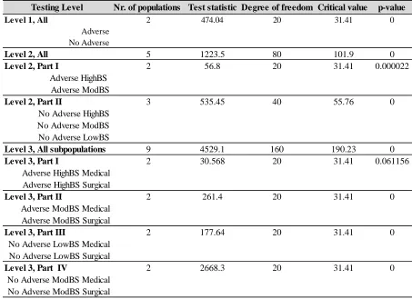
Table 3.6: The Chi-square test results at all three levels for the subpopulations using Alternative #1 (as shown in Figure 3.1). P-values which are less than 0.00001 are denoted as 0... 51
Table 3.7: The Kruskal-Wallis test results for the subpopulations using Alternative #1. A result is not available (n.a.) if a state movement cannot be observed between two states due to the model structure. The blue highlighted cells indicate p-values above 0.05. ... 56
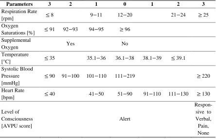
Table 4.1: Elements of NEWS, Royal College of Physicians, 2012. ... 66
Table 4.2: SMDP model parameters. ... 72
Table 4.2: NEWS, corresponding model states, and the clinical interpretation of the states. 74 Table 4.3: The indicator cost variable, 𝑐𝑠, 𝑗. ... 81
Table 4.5: Case study patient subpopulation characteristics. ... 103
Table 4.6: Optimal policy by subpopulation... 104
Table 5.1: Input parameters for the distribution of 𝜌(s). ... 123
Table 5.2: Distributions of perception measure 𝜉(s). ... 124
Table 5.3: Clustering parameters for calculating the distance between clusters. ... 130
LIST OF FIGURES
LIST OF ABBREVIATIONS
Adv Adverse event
APD Acute and persistent physiological deterioration BSS Braden skin score
CCC Computing Community Consortium
CD4 Cluster of differentiation four EMRs Electronic medical records
EWSs Early Warning Scores
FMEA Failure Modes and Effect Analysis
FTR Failure to rescue
GEE Generalized estimating equations GLM Generalized linear model
HighBS High Braden skin score ICU Intensive care unit
IHI Institute for Healthcare Improvement IOM Institute of Medicine
IPFS Inpatient Physiological Failure Score LowBS Low Braden skin score
MDP Markov decision process
MEWS Modified Early Warning Score MLEs Maximum likelihood estimates ModBS Moderate Braden skin score NAE National Academy of Engineering NEWS National Early Warning Score
NEWSDIG National Early Warning Score Design and Implementation Group No Adv No adverse event
NRC National Research Council
PCAST President’s Council of Advisors on Science and Technology RCPL Royal College of Physicians, London
ROD Risk of deterioration RRT Rapid response team
SMDP Semi-Markov decision process SPC Statistical process control
TTS Time to stabilization
Chapter 1
1.
Introduction
The transformation of health care from reactive and disease-centered to proactive and patient-centered care has been an emerging focus of hospitals worldwide. This transformation is associated with challenges, particularly the challenge of realizing the full potential of electronic medical records (EMRs). Despite innovations in health information technology, the use of EMRs to support clinical decision making has not met expectations (Kohn et al., 1999). The need for a systematic approach to enhance the performance of patient-centered medical care has been recognized by organizations such as the President’s Council of Advisors on Science and Technology (PCAST), the National Research Council (NRC), the Institute of Medicine (IOM), the Computing Community Consortium (CCC), and the National Academy of Engineering (NAE).
illness, or the treatment received during recovery from a surgery. The general ward refers to rooms occupied by one or more individuals during a stay in the hospital who do not require close observation and high intensity medical care, i.e., the patients are not monitored continuously.
ADP is identified by acute and persistent disturbance in physiological measures, such as heart rate and blood pressure (Kyriacos et al., 2011; Peberdy et al., 2007). Hospitals have recognized the importance of timely interventions by a team with critical care competencies to prevent APD, or minimize the decline in health in case of APD. A medical emergency team, also called a Rapid Response Team (RRT), is a specialized team of clinicians who provide on-site critical care service for physically deteriorating individuals who are being treated outside of an ICU (Leape et al., 1991; Searle et al., 2008; Subbe et al., 2001; Winters et al., 2007).
The research described in this dissertation was performed in collaboration with the Division of Health Care Policy & Research, Department of Health Sciences Research, Mayo Clinic. The main motivation is to address failure to recognize or late response to APD, and support care providers by RRT activation decisions. A multidisciplinary team, including over 700 physicians and nurses at Mayo Clinic, conducted a Failure Modes and Effect Analysis (FMEA) in December 2012, and identified 33 reasons for delayed or failed response to APD using: (i) frequency of occurrence, (ii) severity of impact to the patient, and (iii) ease of detecting the failures at the moment they occur. The FMEA results showed that the lack of a standard definition for APD, and the heterogeneous patient population are the primary factors causing delayed or failed response to APD. These results motivated our research. The research described in this dissertation focuses on patients in the general ward. Studies indicate that irregular monitoring patterns in the general ward may delay recognition of a deteriorating patient (Mitchell et al., 2010; Subbe et al., 2001).
patient’s clinical condition (Bynd et al., 2004; Gray et al., 2002). EWSs not only provide a
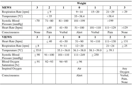
standardized method for clinical assessment, they also suggest which patients may require attention outside of an ICU provided by an RRT. Widely used EWSs are the Modified Early Warning Score (MEWS), the VitalPAC Early Warning Score (VIEWS), and the National Early Warning Score (NEWS) (Prytherch et al., 2010; Royal College of Physicians, 2012; Subbe et al., 2001). These EWSs differ in their physiological measures, and in the thresholds for triggering a response, e.g., RRT activation.
Table 1.1: Commonly used warning scores: MEWS and VIEWS.
Weight
MEWS 3 2 1 0 1 2 3
Respiration Rate [rpm] < 9 9−14 15−20 21−29 > 29 Temperature [ºC] < 35 35−38.4 >38.4
Systolic Blood Pressure [mmHg]
<70 71−80 81−100 101−199 >199
Heart Rate [bpm] <40 41−50 51−100 101−110 111−129 >129 Consciousness None Pain Verbal Alert Verbal Pain None
VIEWS 3 2 1 0 1 2 3
Heart Rate [bpm] < 40 41−50 51−90 91−110 111−130 > 131 Respiration Rate [rpm] < 8 9−11 12−20 21−24 > 25 Temperature [ºC] < 35.0 35.1−36.0 36.1−38.0 38.1−39.0 > 39.1
Systolic Blood Pressure [mmHg]
< 90 91−100 101−110 111−249 > 250
Blood Oxygen Saturation [%]
< 91 92−93 94−95 > 96
Inspired Oxygen Air Any
Oxygen
Consciousness Alert Verbal,
Pain, None
aggregate score exceeding a fixed threshold suggests immediate clinical assessment, and RRT activation, regardless of the patient characteristics (Royal College of Physicians, 2012). Table 1.2 shows the current RRT activation criteria which are used at Mayo Clinic for all adult patients. Bedside care providers at Mayo Clinic are encouraged to activate RRT if at least one of these criteria is satisfied.
Table 1.2: RRT activation criteria at Mayo Clinic.
Criteria Explanation
1 A staff member is worried about the individual
2 Acute and persistent declining oxygen saturations < 90 [%]
3 Acute and persistent change in heart rate < 40 or >130 [bpm]
4 Acute and persistent change in systolic blood pressure < 90 [mmHg]
5 Acute and persistent change in respiration rate < 10 or > 28 [rpm]
6 Acute chest pain suggestive of ischemia
7 Acute and persistent change in conscious state
8 New onset of symptoms suggestive of stroke
RRT activation criteria in Table 1.2 include subjective elements, e.g., “being worried.” In addition, the criteria are not patient-specific, e.g., one patient’s systolic blood pressure may deviate from the predetermined normal range without indicating APD, and for another patient the same measure may be life-threatening. Thus, the current RRT activation criteria at Mayo Clinic may result in suboptimal resuscitation interventions.
same hospital, the EWSs may be implemented without considering the patient characteristics. Exploring the relationship between patient characteristics and APD, and identifying the patient groups who may benefit from an increased level of acute medical care would provide guidance in RRT activation. Developing analytical models based on EWSs has the potential to better inform and personalize resuscitation decisions by presenting the physiological deterioration over the hospitalization period as a stochastic process, and by identifying patients-specific resuscitation rules. From the modeling perspective, EWSs have several advantages: (i) EWSs can be easily computed from EMRs, (ii) the aggregate score combines several dimensions of health, which are informative for detecting APD; and (iii) EWSs can help to monitor the changes in physiological condition over time.
1.1 Problem Description
The current acute care delivery at Mayo Clinic can be improved by using EMRs to inform and personalize resuscitation decisions. The challenge is to use the large amount of EMRs in an efficient way to support the resuscitation decisions, such as the RRT activation. In this section, we present two dimensions of this challenge: the challenge of determining patients at risk of deterioration, and the need for dynamic models.
1.1.1 Challenge of Determining the Patients at Risk of Deterioration
is challenging, because the patients are not monitored continuously.
EWSs are widely used to identify patients at risk of APD and trigger resuscitation decisions, e.g., RRT activation (Escobar et al., 2012; Kyriacos et al., 2011; Smith et al., 2006). The performance of any score depends on the patient population. Using the same thresholds for all patients may result in activating RRT unnecessarily. RRT commonly provides critical care in the ICU until any activation occurs. In case of an RRT call, the team provides on-site care in the general ward. The time RRT spends in transit and for the evaluation of patients who do not require this level of care translates to wasted resources, which could be used more appropriately to serve patients who are in need. Decision analytical models can transform EMRs into a decision model to inform RRT activation decisions.
An important feature of a decision analytical model is its interpretability. Interpretability is the ease with which a concept or a result can be understood. Although interpretability is subjective, analytical decision models aim to provide feedback which is easy to implement in practice (Cohen et al., 1980). A good example of an interpretable model is one which provides a control-limit policy. A control-limit policy is a set of decision rules with predetermined threshold value(s). In the problem context, an example could be: “if the current warning score observation 𝑥 is above (or below) the threshold, then initiate RRT; else, wait until the next observation.” Such a policy would be preferred in clinical practice due to its simplicity and interpretability.
1.1.2 Need for Dynamic Models
data represent underlying physiological processes. In this context, a patient’s health can be considered a dynamic, stochastically failing and improving system. Some scores fail to capture the dynamic nature of the patient’s health by using a one-time measure to evaluate the risk of deterioration during hospitalization (Gray et al., 2002). If the EWSs are collected repeatedly, they can provide information about the changes in a patient’s physiology more dynamically. A dynamic programming model offers a suitable approach to capture this probabilistic system with repeatedly collected EWSs, because a patient’s health condition changes dynamically and stochastically during the hospitalization.
One advantage of a dynamic programming model, such as a Markov decision process (MDP) model, is that multi-stage problems can be solved by analyzing a sequence of simpler, recursively defined decision problems, e.g., a patient’s hospitalization can be analyzed as sequential stages. MDP models are appropriate for capturing the dynamic nature of a patient’s health and resuscitation decisions triggered by the health condition. An MDP model is a sequential decision model obtained by using a set of possible actions, a set of immediate rewards (or costs) associated with the current state and action, and a terminal reward (or cost) where the state transitions follow a Markov chain (Puterman, 1994). In an MDP, a decision maker can influence the behavior of a probabilistic system through his/her actions as the system evolves through time. The Markov property in our problem context states that a patient’s future health state depends only on the current state and the current resuscitation
states resulting from the actions.
1.2 Research Question
With the goal of developing a patient-centered, dynamic, and interpretable decision model, we seek to answer the following research question: “How can we use EMRs efficiently to optimize patient-centered resuscitation decisions of care providers prior to and during APD in adult patients, while considering the care provider resource use?” Further relevant questions are:
Which patient characteristics can be used to classify statistically significantly different subpopulations? (Chapter 3);
Are there optimal policies with patient-specific EWS thresholds? (Chapter 4);
What are the total expected costs associated with health states? (Chapter 4);
Under which conditions do optimal value functions have special structural properties? (Chapter 4); and
1.3 Remaining Content of the Dissertation
Chapter 2
2.
Literature Review
This chapter gives an overview of the existing literature regarding Markov decision process (MDP) and semi-Markov decision process (SMDP) models, and a range of their applications. In this chapter, we review the medical and engineering literature that is relevant for our research. We discuss similarities and differences between the existing studies and our research. In Sections 2.1 and 2.2, we provide an overview of MDP models and their applications in health care. Section 2.3 focuses on SMDP models. Section 2.4 summarizes studies that applied SMDP models to machine maintenance, queuing, financial decision making problems, and health care. We conclude in Section 2.5.
2.1 Markov Decision Process
state of the system and the action selected by the decision maker in the current state (Puterman, 1994). Any decision made at each step affects both the transition probabilities and the rewards obtained upon leaving the present state. The challenge is to specify a sequence of actions which allows the system to perform optimally by predetermined success criteria, e.g., maximizing the total expected rewards or minimizing the total expected costs. In the remainder of this section, we provide an overview of the undiscounted, finite-horizon MDP model. For further details about MDP formulations and solution techniques, the reader is referred to Howard (Howard, 1971), Ross (Ross, 1970) and Puterman (Puterman, 1994).
A finite-horizon, discrete-time MDP can be formulated as a collection of the objects:
(𝑆, 𝐴𝑠, 𝑇, 𝑃𝑡(𝑠, 𝑑(𝑠)), 𝑟𝑡(𝑠, 𝑑(𝑠)))
where 𝑆 = {1, 2, … } represents the state space including all possible states the system can occupy, 𝐴𝑠the action space including all possible actions in state 𝑠 ∈ 𝑆, 𝑇 the set of decision
epochs 𝑡 = {1,2, … , 𝑁} indicating points in time when actions are allowed with 𝑁 < ∞,
𝑃𝑡(𝑠, 𝑑(𝑠)) the transition probability matrix conditional on current state 𝑠 and action 𝑑(𝑠), and
𝑟𝑡(𝑠, 𝑑(𝑠)) the reward (or cost) associated with state 𝑠 ∈ 𝑆, and action 𝑑(𝑠) ∈ 𝐴𝑠. This is a “Markovian” model, also called a memoryless model, because the transition probabilities and
reward functions depend on the past only through the current state of the system and action. A decision rule, denoted by 𝑑𝑡(𝑠), determines a procedure for selecting an action in each state at a specified decision epoch 𝑡, 𝑑𝑡(𝑠): 𝑆 → 𝐴𝑠. A policy, denoted by 𝜋 = (𝑑0(𝑠), 𝑑1(𝑠), … ), is a
if 𝑑𝑡(𝑠) = 𝑑(𝑠) ∀ 𝑡 ∈ 𝑇, and 𝑠 ∈ 𝑆. For a maximization problem, the expected total reward
over the decision making horizon if policy 𝜋 is used given the initial state 𝑠 at the first decision epoch is
𝑣𝑁(𝑠) = 𝐸𝑠𝜋{∑𝑁−1𝑡=1 𝑟𝑡(𝑠𝑡, 𝑑𝑡(𝑠𝑡)) + 𝑟𝑁(𝑠𝑁)},
where 𝑟𝑁(𝑠𝑁) is the terminal reward obtained by the end of the horizon when the system
reaches state 𝑠𝑁 (Puterman, 1994).The objective of an MDP is to find the policy 𝜋∗ from the
set of Π, i.e., the set of all possible policies, which maximizes the expected total reward or
minimizes the expected total cost for each 𝑠 ∈ 𝑆. The optimal value function at each state and decision epoch can be solved recursively by using backwards induction, which uses the recursive relationship of dynamic programming. Further details about backwards induction can be found in Howard (Howard, 1971).
2.2 MDP Applications in Health care
Further, they suggest Markov models for clinical decision making as an alternative to decision trees. Their study is followed by continuous growth in the number of MDP models for medical decision making.
Shechter et al. develop a finite-horizon MDP model to determine the optimal time to initiate HIV treatment with the goal of maximizing a patient’s total expected quality-adjusted
Optimal decisions are identified based on the perceived risk of different stages of breast cancer. Their results suggest that screening should start relatively early in life, and continue relatively late in life regardless of different screening intervals.
These studies represent a small selection of the wide applications of MDP models in health care. Although our research does not model a chronic disease, such as HIV or breast cancer, we seek to contribute to the literature regarding the Markovian models with health care applications by modeling the stochastic evolution of the acute physiological deterioration of a patient during hospitalization.
2.3 Semi-Markov Decision Process
A semi-Markov decision process (SMDP), also called Markov Renewal Program, is a generalization of MDP model. SMDP models allow the time between state transitions to follow an arbitrary distribution. SMDP models were first studied by Levy, Smith and Takacs in 1954 (Jewell, 1963a; Jewell, 1963b). Jewell and Howard introduced solution algorithms for finite- and infinite-horizon SMDP models (Howard, 1971; Jewell, 1963b). For further details about SMDP solution techniques, the reader is referred to Ross (1970), Cinlar (1975), and Puterman (1994).
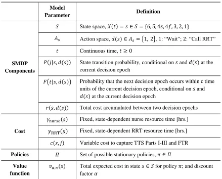
(𝑆, 𝐴𝑠, 𝑇, 𝑃(𝑗|𝑠, 𝑑(𝑠)), 𝐹(𝑡|𝑠, 𝑑(𝑠)), 𝑟(𝑠, 𝑑(𝑠)))
where 𝑆 represents the state space including all possible states the system can occupy, 𝐴𝑠the action space including all possible actions in state 𝑠 ∈ 𝑆, and 𝑇 the set of decision epochs with
𝑇 = {1,2, … , 𝑁} where 𝑁 ≤ ∞, 𝑃(𝑗| 𝑠, 𝑑(𝑠)) the probability that the embedded MDP is in state
𝑗 at the next decision epoch given that the action 𝑑(𝑠) is taken in state 𝑠 at the current decision
epoch. The term 𝐹(𝑡|𝑠, 𝑑(𝑠)) denotes the probability that the next decision epoch occurs within
𝑡 time units of the current decision epoch, given that the current state is 𝑠 and the decision
maker selects action 𝑑(𝑠). This is also called the sojourn time distribution, or holding time distribution. The term 𝑟(𝑠, 𝑑(𝑠)) is the cost (or reward) accumulated between two decision epochs given the state at the current decision epoch 𝑠 ∈ 𝑆, and action 𝑑(𝑠) ∈ 𝐴𝑠.
In SMDP models, the action choice determines the joint probability distribution of the subsequent state and the time between decision epochs. The system evolves as follows:
system occupies 𝑠 ∈ 𝑆 at some decision epoch;
decision maker selects an action 𝑑(𝑠) from the set 𝐴𝑠;
the next decision epoch occurs at or before time 𝑡 and the system is in state 𝑗 at that decision epoch with probability 𝑄(𝑡, 𝑗|𝑠, 𝑑(𝑠)) where
𝑄(𝑡, 𝑗|𝑠, 𝑑(𝑠)) = 𝑃(𝑗|𝑠, 𝑑(𝑠)) 𝐹(𝑡|𝑠, 𝑑(𝑠)).
decision epochs only is the embedded Markov decision process, also called the semi-Markov decision process. The natural process and the semi-Markov decision process overlap at decision epochs (Figure 2.1).
State of the System
Time
Decision epoch
Decision epoch
Decision epoch
s = 1 s = 2 s = 3
Decision epoch
Figure 2.1: Sample path of an SMDP with three states, S={1,2,3}. The solid lines denote the natural process. Closed circles indicate that the natural process is right-continuous. Open circles denote the
state of the SMDP at decision epochs (i.e., semi-Markov decision process) (Puterman, 1994).
SMDP models are classified as finite- or infinite-horizon models; discrete-time or continuous-time models; and discounted or undiscounted models. In a finite-horizon SMDP the system is allowed to operate only for a finite period of time, e.g., 𝑇 = {1,2, … , 𝑁} with 𝑁 < ∞. In an infinite-horizon model the system can operate indefinitely, i.e., 𝑇 = {1,2, … }. In a
positive time spent in a state, i.e., 𝐹(𝑡|𝑠, 𝑑(𝑠)) is a continuous distribution.
In infinite-horizon SMDP models the optimal policy is time-independent, or stationary. A stationary policy 𝜋 = (𝑑(1), 𝑑(2), … ) determines a decision rule 𝑑(𝑠) for each state independent of the time. Following the policy 𝜋, the expected total cost is
𝑣𝛼𝜋(𝑠) = 𝑟(𝑠, 𝑑(𝑠)) + ∑ ∫ 𝑒−𝛼𝑡𝑄(𝑑𝑡, 𝑗|𝑠, 𝑑(𝑠)) 𝑣 𝛼𝜋(𝑗) ∞
0 𝑗∈𝑆
(2.1)
where
𝑟(𝑠, 𝑑(𝑠)) = 𝛾(𝑠, 𝑑(𝑠)) +
∫ ∑ [∫ 𝑒𝑢 −𝛼𝑡
0 𝑐(𝑗, 𝑠, 𝑑(𝑠)) 𝑃(𝑗|𝑡, 𝑠, 𝑑(𝑠))𝑑𝑡]𝐹(𝑑𝑢|𝑠, 𝑑(𝑠)) 𝑗∈𝑆
∞
0 .
In Equation (2.1), 𝛾(𝑠, 𝑑(𝑠)) denotes the immediate fixed cost associated with being in state 𝑠
and taking action 𝑑(𝑠); 𝑐(𝑗, 𝑠, 𝑑(𝑠)) is the cost rate capturing the cost collected between two decision epochs, discounted to the current time using continuous discounting 𝑒−𝛼𝑡 and 𝛼 > 0.
Table 2.1: Policy iteration algorithm for infinite-horizon SMDP.
Step 1: Initialization. Set 𝑛 = 0, and select an arbitrary stationary policy 𝑑𝑛=
(𝑑𝑛(1), 𝑑𝑛(2), … ) ∈ 𝐷 where state space is denoted by 𝑆. Step 2: Policy Evaluation. Solve 𝑣𝛼𝑑𝑛= (𝐼 − 𝑀𝑑𝑛)
−1
𝑟𝑑𝑛 to evaluate the initial policy, and
obtain the value function vector 𝑣𝛼𝑑𝑛.
Step 3: Policy Improvement. Choose 𝑑𝑛+1∈ argmin𝑑𝑛∈𝐷 {𝑟𝑑𝑛+ 𝑀𝑑𝑛𝑣𝛼𝑑𝑛}. Set 𝑑𝑛+1= 𝑑𝑛 if possible.
Step 4: Termination. If 𝑑𝑛+1= 𝑑𝑛 , stop. Set 𝑑∗= 𝑑𝑛. Otherwise, increment 𝑛 by 1, return to step 2.
In policy iteration algorithm, the infinite-horizon problem is solved by searching among the possible stationary policies 𝐷 to find the optimal policy 𝑑∗. After selecting an arbitrary initial stationary policy 𝑑𝑛 for the iteration 𝑛 = 0, the policy is evaluated by
computing the value function for each state, 𝑣𝛼𝑑𝑛(𝑠), which is expressed in matrix-vector
notation as
𝑣𝛼𝑑𝑛 =𝑟
𝑑𝑛+𝑀𝑑𝑛𝑣𝛼
𝑑𝑛.
The term 𝑀𝑑𝑛represents the joint probability of the state movement and the holding time
distribution if the policy 𝑑𝑛 is followed. The (𝑠, 𝑗) element of the |𝑆| × |𝑆| matrix 𝑀𝑑𝑛 are
𝑚𝑑𝑛(𝑗|𝑠,𝑑𝑛(𝑠)) = ∫ 𝑒
−𝛼𝑡 ∞
0
𝑄𝑑𝑛(𝑑𝑡, 𝑗|𝑠,𝑑𝑛(𝑠)) for 𝑗, 𝑠 ∈ 𝑆 and 𝑑𝑛(𝑠)∈ 𝐴𝑠.
case, the algorithm terminates, and the optimal stationary policy and the corresponding value function realization are found.
By definition of 𝑀𝑑𝑛, the rows may not sum to one. Ross contributed an assumption for
addressing this issue as follows (Ross, 1970):
Assumption 3.1. There exists 𝜀 > 0 and 𝛿 > 0 such that 𝐹(𝛿|𝑠, 𝑑(𝑠)) ≤ 1 − 𝜀 for all 𝑠 ∈ 𝑆, 𝑑(s) ∈ 𝐴𝑠.
Assumption 3.1 avoids the possibility of an infinite number of decision epochs within a finite time, and ensures that for any given policy the row sums of 𝑀𝑑𝑛 are strictly less than 1. If
‖𝑀𝑑𝑛‖ < 1, then (I −𝑀𝑑𝑛)−1 exists (as described in Appendix A). If (I −𝑀𝑑𝑛)−1 exists, then
the value function at the 𝑛𝑡ℎiteration is computed as (Puterman, 1994):
𝑣𝛼𝑑𝑛 =𝑟
𝑑𝑛+𝑀𝑑𝑛𝑣𝛼𝑑𝑛 ↔ 𝑣𝛼𝑑𝑛 = (I −𝑀𝑑𝑛) −1
𝑟𝑑𝑛 .
2.4 SMDP Applications
This section gives a brief overview of SMDP applications in the literature. We focus on selected work relevant to our study.
2.4.1 SMDP Applications in Machine Maintenance
Kao developed a finite-state discrete-time semi-Markov decision process model with two actions, repair or do nothing (Kao, 1973). It was assumed that without an intervention (repair) the system can only remain in its current state or deteriorate, a repair returns the system to the best possible state from every state, and once system reaches the worst state the only possible action is to repair. Kao provides state-dependent, dependent, or state- and age-dependent optimal replacement rules using policy iteration. In addition, Kao provides conditions for the existence of a control-limit replacement rule which states that when the system reaches the control-limit state, the rule dictates to replace the machine for any state greater or equal to the threshold state. The aspect of a stochastically failing system is similar to our approach of modeling physiological deterioration. Our model differs from Kao’s in two aspects: (i) patients can recover, therefore the system can fail or improve stochastically with or without intervention; and (ii) we do not assume that activating RRT returns the patients’ health status to the best possible state from every state with certainty. We discussed Kao’s study in detail because of its similarities to our research, such as establishing conditions for the existence of a control-limit decision rule. There are several other examples of semi-Markovian deterioration models in the literature (Lam & Yeh, 1994; Kim & Makis, 2009).
2.4.2 SMDP Applications in Queuing
horizon models. SMDP models allow general arrival times, or general service time distributions. They can be used to analyze G/M/c and M/G/c queuing systems. Optimal policies can be considered from the societal perspective, e.g., optimizing total expected rewards for the entire population served, or from an individual’s perspective.
Stidham developed a SMDP model to determine individually and societally optimal entering policies for a G/M/1 model for finite- and infinite-horizon problems with and without discounting (Stidham, 2005). He showed that the societally optimal policy is a monotone policy: a customer is less likely to be accepted as the number of customers already in the system increases. Individually optimal policies result in allowing more customers to enter, who would not be allowed to enter in the socially optimal policies. These properties are shown to hold both for finite- and infinite-horizon problems. There are differences between our SMDP model and Stidham’s models. In Stidham’s study there are two actions “admit” and “reject,” and
decisions are only made at arrival times. In the finite-horizon case, assuming that (i) the system will shut down after 𝑛 customers are served, (ii) there are currently 𝑖 customers in the system, (iii) an arriving customer will provide the reward 𝑟 if accepted into system, and (iv) the discount factor is 𝛼 > 0, the optimal value function is:
𝑣𝑛,𝛼(𝑖, 𝑟) = max {𝑟 + 𝑈𝑛,𝛼(𝑖 + 1) 𝑖𝑓 𝑎 = 𝑎𝑐𝑐𝑒𝑝𝑡
𝑈𝑛,𝛼(𝑖) 𝑖𝑓 𝑎 = 𝑟𝑒𝑗𝑒𝑐𝑡 }, (2.2)
where 𝑈𝑛,𝛼(𝑖 + 1, 𝑟) denotes the total expected discounted reward over the entire planning
the existence of a monotone optimal policy using this property, and shows that as the number of customers in the system increases, an arriving customer with reward 𝑟 is more likely be rejected. Although we also consider two actions, “activate RRT” and “wait,” proving structural properties in our case is more challenging, because the patient can move to any health state following an action.
2.4.3 SMDP Applications in Finance
Another application area for SMDP models is in financial decision making. In financial decision problems, a common approach is the optimal stopping time framework. Optimal stopping problems commonly include two actions: one action immediately stops the process; the other action allows waiting until next decision epoch. The waiting action commonly generates cost during the waiting time. The goal is to maximize the total expected reward, or minimize the total expected cost, until the process has terminated. Lippman and McCall used optimal stopping for optimal job search (Lippman & McCall, 1976). Mamer focused on the problem of optimally liquidating an asset by a fixed deadline using a finite-horizon SMDP with optimal stopping time structure (Mamer, 1986). Mamer assumed that the amount of an arriving offer follows a distribution 𝐹0(∙); the time between offers follows the distribution 𝐺(∙);
deterioration process can be modeled as an optimal stopping time problem if calling RRT terminates the decision process, e.g., if RRT calls are always followed by an ICU transfer or discharge from general ward. In this case, the action “wait” would correspond to postponing the decision until next observation is available.
2.4.4 SMDP Applications in Health care
Our study shares similarities with Kao’s model, such as using transient recovery states and the combination of alive and deceased discharge dispositions as a single absorbing state, and creating subpopulations using patient characteristics, which will be discussed in Chapter 3. The main differences between Kao’s and our model are related to updating of the model parameters. Kao uses the additional information obtained as the patients move through the recovery system to update the state transition probabilities. In our model, the state transition probabilities are estimated from EMRs and are not updated. In addition, Kao does not test the underlying model assumptions using statistical tests. The similarity between our study and Weiss et al.’s is that we use statistical tests, Chi-square test and the Kruskal-Wallis test, to determine if the patient subpopulations are statistically significantly different.
2.5 Contributions of this Dissertation
length of stay in each state; and (iv) finally conduct statistical analysis by using (a) the Chi-square test to determine if any given set of transition probability matrices differ significantly, and (b) the Kruskal-Wallis test to determine if the holding times for the corresponding subpopulations are drawn from the same distribution. In Chapter 4, we model the stochastic progression of APD and the recovery process with two control alternatives: wait or call RRT. We analyze 24-months of EMRs to represent the deterioration and recovery process of hospitalized patients, and develop an SMDP model. The findings highlight the importance of personalized resuscitation by identifying subpopulation-specific RRT triggers, and provide the expected total cost for each subpopulation. Further, we provide insight into the structural properties, and present the conditions for existence of the monotone optimal policies for a stochastically deteriorating and improving system. In Chapter 5, we address the uncertainty in model cost parameters. The fixed cost parameters, representing the nurse and RRT time based on a patient’s physiological condition, are derived from EMRs, and are subject to errors. In addition, the care provider team in the general ward may be heterogeneous, and provider time may be evaluated differently based on the expertise level and the intensity of care. We develop a model which allows the care providers to assign weights, as random variables, to the cost function with average fixed costs, and to a conservative cost function with the maximum fixed costs. Further, we include a relative RRT resource perception measure as a random variable. We explore the changes in model results due to the variation in the fixed costs for a selected subpopulation.
Chapter 3
3.
Identification of Patient Populations Using
Early Warning Scores
3.1 Introduction
and provide a RRT response triggering structure, as discussed in Chapter 1. However, the current RRT criteria include subjective elements, and the triggers are used without considering patient-specific characteristics. EWSs can be derived from electronic medical records (EMRs), and they can enhance the personalization of the resuscitation process by identifying different patient populations. The performance of any EWSs-based resuscitation process may depend on the patient type. For example, Capan and Ivy (2013) compared the performance of EWSs in predicting future deterioration events using two vital-sign related indicators, shock index and mean arterial pressure. Their study showed the predictive decision tool’s performance varied depending on patient characteristics.
In this chapter, we segment the EMRs to identify homogeneous patient groups as the first step in individualizing the acute care decision making process. We hypothesize that the hospitalized patient population is heterogeneous, and seek to identify medically relevant and statistically significantly different subgroups, denoted as subpopulations, using patient characteristics. The remainder of this chapter is organized as follows: in Section 3.2, we provide an overview of the relevant literature. In Section 3.3, we present our methodology, including the semi-Markov process, classification of the subpopulations, and the statistical tests for the subpopulations. We conclude in Section 3.4.
3.2 Literature Review
maintenance literature (Kim & Makis, 2009; Lam & Yeh, 1994; Love et al., 2000; So, 1992). Machine maintenance models typically analyze deteriorating industrial machinery, which is commonly modeled as a stochastically failing system. A replacement may return the system to the initial state; a repair may bring the system to a more desirable state. The objective is to obtain optimal decision rules that minimize costs associated with decreased machine performance and repair. In our problem context, the multi-state stochastically evolving system is the patient’s physiological condition. The EWSs are used to observe the deteriorating and improving physiological condition.
mean and variance which may not be appropriate for modeling health measures, such as vital signs, which fluctuate frequently. In addition, in multivariate SPC charts assignment of causes for an out-of-control observation is only possible once an unusual event has been detected (Kourti & MacGregor, 1996). In our problem context, by the time the out-of-control observation occurs, it may be too late to initiate resuscitation decisions. Therefore, SPC charts are more suitable for routine monitoring purposes to check process stability, rather than acute care decision support.
hospitalization experience can be determined using the patient ID numbers. Similar to Kao’s model, we also use transient states to capture the recovery and deterioration conditions, and an absorbing state to represent discharge including several discharge dispositions, e.g., alive and deceased (Kao, 1972). Our study differs from Kao’s in the information updating aspect. Kao (1972) used the additional information obtained as the patients move through the recovery system, and updated the state transition probability estimates conditional on the time a patient spends in the current state. In our model, the state transition probabilities are estimated from EMRs, and are not updated.
3.3 Methodology
a state transition occurs, i.e., holding time, for each subpopulation. The state transition probabilities and the holding time observations are used to determine if the subpopulations differ statistically significantly.
3.3.1 Model Formulation
A semi-Markov process is a dynamic probabilistic system in which successive state occupancies are determined by the transition probabilities of a Markov process, but the length of stay in any state is a random variable, which depends on the current state and on the state to which the next transition will be made (Howard, 1970). A semi-Markov process makes transitions between states 𝑠 ∈ 𝑆, where 𝑆 represents the set of all possible states. When the system enters state 𝑠, the next state 𝑗 is determined according to the transition probability
𝑃(𝑗|𝑠) which denotes the probability that the process which entered state 𝑠 ∈ 𝑆 on the current
transition will enter the state 𝑗 ∈ 𝑆 on the next transition. The transition probabilities satisfy
𝑃(𝑗|𝑠) > 0 and ∑𝑗∈𝑆𝑃(𝑗|𝑠) = 1for all 𝑠 ∈ 𝑆. When the system enters state 𝑠, the system holds
for a random amount time in state 𝑠 before making a transition to state 𝑗. 𝐹(𝑡|𝑠, 𝑗) denotes the probability that the holding time is less than or equal to 𝑡 time units conditional on the current state 𝑠, and subsequent state 𝑗. Semi-Markov process models are classified as discrete-time or continuous-time. In a discrete-time model, state movements are on a fixed time scale, i.e., 𝐹 is a discrete distribution. In a continuous-time model, the state transitions can occur after any positive time spent in a state, i.e., 𝐹 is a continuous distribution.
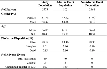
and recovery of adult patients in the general ward. The study population includes adult patients hospitalized at Mayo Clinic in the general ward during January 2010. Inclusion criteria include age at admission (≥18 years), and care location (observations collected during a stay in the general ward). Table 3.1 summarizes the study population characteristics.
Table 3.1: Patient population characteristics, derived from January 2010 EMRs.
Study Population
Adverse Event Population
No Adverse Event Population
# of Patients 2573 105 2468
Gender [%]
Female 51.73 47.62 51.90
Male 48.27 52.38 48.10
Age
Mean 56.85 61.77 56.64
Std. 18.43 15.11 18.54
Discharge Disposition [%]
Alive 98.14 93.40 98.30
Hospice 1.01 3.80 0.90
Dead 0.85 2.80 0.80
# of Adverse Events
RRT activation 40 40 0
Code45 3 3 0
Unplanned transfer to ICU 169 169 0
from the patients without an adverse event experience. As shown in Table 3.1, we segment the study population into two groups: patients who have not experienced an adverse event during January 2010, and patients who have had at least one adverse event during January 2010. Although the two groups do not differ significantly in age and gender distribution, there is a significant difference in the discharge disposition distribution. For example, the percentage of patients discharged dead is four times larger in the adverse-event population than in the adverse-event population (2.80%, and 0.80%, respectively). In addition, only 0.90% of the no-adverse-event population was discharged to hospice, compared to 3.80% in the no-adverse-event population. Further, Table 3.1 shows that the most common adverse event is the unplanned transfer to the ICU, followed by the RRT activation. The least common adverse event is Code45, which is an extreme measure only activated if a patient’s respiration or cardiovascular system stops functioning. These results should be interpreted with care, because we analyze one month of EMRs, and the distribution of adverse events may be different in another month.
We use MEWS to represent the states, i.e., the patient’s physiological condition. Table 3.2 illustrates the model states and the corresponding MEWS, and the discharge state.
Table 3.2: State space definition using MEWS.
MEWS Model State
{0, 1}
1 (stable) or 2 (returned to stable after
deterioration)
2 3
{3, 4} 4
≥5 5
State 1 represents the desired “stable” health state. States 1 and 2 distinguish a stable patient,and a patient who has been stabilized following significant deterioration (i.e., MEWS >1). Based on medical expert opinion, MEWS ≥5 is considered a “distress” state which may have severe health consequences for the patient. The absorbing state 6 includes all outcomes which result in the patient leaving the general care setting, including transfer to a higher level, discharge from the hospital, and patient death. The differentiation between states 1 and 2 represents the difference in physiological condition for a patient who has never had an elevated MEWS value, and a patient who has experienced an elevated MEWS value and returned to MEWS 0 or 1. The differentiation between the stable and stabilized states is an important concept in determining a cost structure and the control alternatives in Chapter 4.
3.3.2 Identification of Subpopulations
Table 3.3: Braden skin score as a patient subpopulation criteria.
Score value Patient classification
> 23 LowBS
12−23 ModBS
< 11 HighBS
In the longitudinal data, repeated measures of the same variables are taken for each patient. Multiple measurements of a variable on the same patient are more likely to be correlated, which can cause within-patient correlation of measurements. Further, the number of observations may differ for each patient. Due to differences between patients, if left uncontrolled, the between-patient variation may become part of the experimental error. This may increase the mean square error, and make the detection of real differences between the covariates difficult. Considering the within-patient correlation of measurements, and the between-patient variation, we select a generalized linear model (GLM) to explain the probability of an adverse event (Montgomery, 2008). GLM allows repeated measures and allows the response to follow an arbitrary distribution using a link function 𝑔(. ), e.g., a logit link function:
𝑔(𝑥) = log ( 𝑥 1−𝑥).
In our analysis, the response variable is binary, and is denoted as 𝑌𝑖𝑗 = {0,1} for the ith patient at the jth time point, where 0 corresponds to no adverse event occurrence, and 1 corresponds to
adverse event 𝑃(𝑌𝑖𝑗 = 1), the GLM structure is
log ( 𝑃(𝑌𝑖𝑗 = 1) 1 − 𝑃(𝑌𝑖𝑗 = 1)
) = 𝑋𝑖𝛽 + 𝜀𝑖𝑗
where
𝑖: patient identified by the encounter ID number,
𝑋𝑖: ith row of the fixed effects design matrix including BSS and admission type effects for ith
patient,
𝜀𝑖𝑗: random error of the jth within-individual measurement on the ith patient so that
𝜀𝑖 ≡ [𝜀𝑖1, 𝜀𝑖2, … , 𝜀𝑖𝑛𝑖]𝑇~𝑁𝑛𝑖(0𝑛𝑖, 𝑅𝑖), where 𝜀𝑖 is the 𝑛𝑖× 1 vector of measurements taken on
the ith patient, and 0
𝑛𝑖 is a 𝑛𝑖 × 1 vector of zeros,
𝑅𝑖:𝑛𝑖 × 𝑛𝑖 variance-covariance matrix of within-individual measurements, and
𝑛𝑖: number of observations for ith patient.
We use PROC GENMOD in SAS. This procedure fits models to correlated responses by the Generalized Estimating Equations (GEEs) method. We use five GLMs to explain the probability of an adverse event. The response variable in all five models is 𝑌𝑖𝑗 = {0,1}, as
3=Above 80), and gender (categorical: F=female, M=male) are the explanatory variables. The null hypothesis is that the probability of an adverse event does not depend on MEWS, age, or gender. There is not enough evidence to reject this null hypothesis at the 𝛼 = 5% significance level. Model #3 uses Braden skin score (numerical: [0, 30]) as the explanatory variable. The null hypothesis is that the probability of an adverse event does not depend on Braden skin score. The evidence is sufficient to reject the null hypothesis at the 𝛼 = 5% significance level. Thus, we select Braden skin score as a subpopulation classification criterion. In Model #4, admission type (categorical: general=medical, procedure=surgical) is the explanatory variable. The null hypothesis is that the probability of an adverse event does not depend on admission type. The evidence is sufficient to reject the null hypothesis at the 𝛼 = 5% significance level. We select admission type as another subpopulation classification criterion. Model #5 uses admission type (categorical: general=medical, procedure=surgical), and Braden skin score (numerical [0,30]) as explanatory variables. The null hypothesis is that the probability of an adverse event does not depend on admission type and Braden skin score. The evidence is sufficient to reject the null hypothesis at the 𝛼 = 5% significance level. The results of the five GLMs are summarized in Appendix B.
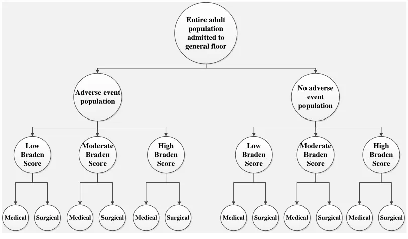
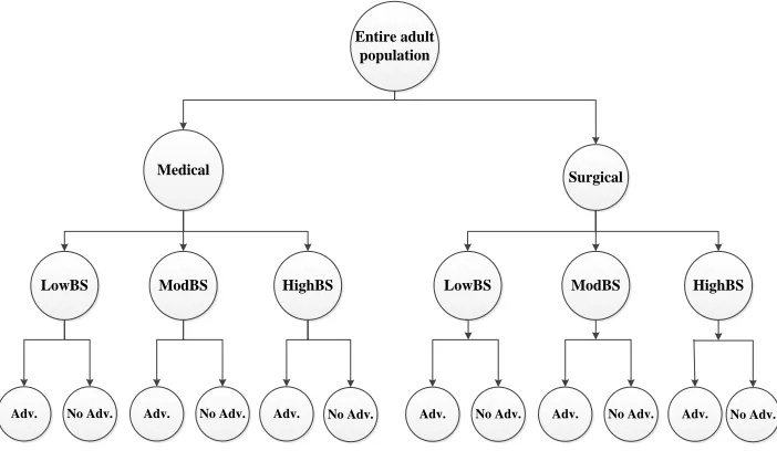
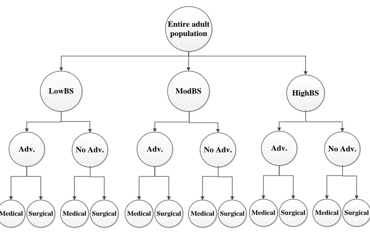
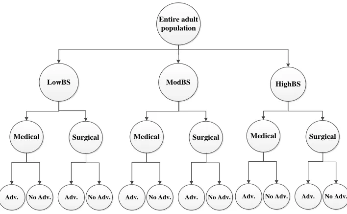
medical expert opinion, suggesting that these populations may be clinically different, and data analysis results, which showed significant difference in the discharge disposition distribution (Table 3.1). The 2nd level is frailty based on Braden skin score categories, as defined in Table 3.3. The 3rd level is the admission type. Figure 3.1 illustrates one alternative for creating subpopulations. Entire adult population admitted to general floor Adverse event population No adverse event population Low Braden Score Moderate Braden Score High Braden Score Low Braden Score Moderate Braden Score High Braden Score
Medical Surgical Medical Surgical Medical Surgical Medical Surgical Medical Surgical Medical Surgical
Figure 3.1: Outline of the subpopulation creation process - Alternative # 1.
3.3.3 Statistical Tests
states that the state transition probabilities are the same. We apply the Chi-square tests to test Hypothesis #1 for various subsets of the subpopulations, e.g., two sets including six populations each with No Adverse and Adverse populations, or various subsets of subpopulations, as discussed in detail later in this section. Before combining any tested subpopulations for which Hypothesis #1 cannot be rejected at the 𝛼 = 5% significance level, it is necessary to determine whether the holding times are drawn from the same distribution (Weiss et al., 1982). We apply the Kruskal-Wallis test to evaluate the null hypothesis that the holding times are drawn from the same distribution, denoted as Hypothesis #2.
Hypothesis #1 and Chi-square Tests
For each subpopulation, we estimate the state transition probabilities using maximum likelihood estimates (MLEs) (Anderson & Goodman, 1957). For any given observation in the EMRs, the state can only be computed if all components of MEWS are measured, which is not the case for all observation entries. The missingness in the data is handled through Last Observation Carry Forward method, i.e., if a component of MEWS is missing, the value is
replaced by the last observed value for the same patient measured in the same visit. Until the
first value of a MEWS component is measured in a given visit, it is considered as missing.
Although Last Observation Carry Forward might not be the best method for data imputation,
in a clinical environment this method is the most realistic way to approach missing data from the care providers’ perspective. This approach represents the process care providers use to analyze patient records if a measurement is missing, and previous measurements of the same
The computation of the MLEs is presented in Appendix C. The MLEs for the state transition probability in the 𝑙𝑡ℎ subpopulation are denoted
𝑝̂𝑖𝑗(𝑙) = 𝑛𝑖𝑗(𝑙) ∑𝑗∈𝑆𝑛𝑖𝑗(𝑙) =
𝑛𝑖𝑗(𝑙)
𝑛𝑖∙(𝑙) for 𝑖, 𝑗 ∈ 𝑆; 𝑙 ∈ {1,2, … ,12}
where 𝑝̂𝑖𝑗(𝑙) is the estimate for the probability of moving from state 𝑖 to state 𝑗 for a patient in
the 𝑙𝑡ℎ subpopulation; 𝑛𝑖𝑗(𝑙) is the number of transitions in subpopulation 𝑙 observed from state
𝑖 to state 𝑗 over the entire observation period; and 𝑛𝑖∙(𝑙) denotes the total number of transitions
in subpopulation 𝑙 that start in state 𝑖.
The Chi-square test is a widely used goodness-of-fit test developed by Pearson which is given by (Conover, 1971)
χ2 = ∑ ∑(𝑂𝑖𝑗− 𝐸𝑖𝑗) 2
𝐸𝑖𝑗 𝑗∈𝑆
𝑖∈𝑆
where 𝑂𝑖𝑗 is the observed count in cell (𝑖, 𝑗) of the subpopulation state transition matrix, and
𝐸𝑖𝑗 is the expected count in cell (𝑖, 𝑗). In this case, 𝑂𝑖𝑗 is equal to 𝑛𝑖𝑗(𝑙), and 𝐸
𝑖𝑗 is equal to 𝑛𝑖∙(𝑙)𝑝̂
𝑖𝑗(𝑙). The test statistic is given by
χ2 = ∑ ∑ ∑ [𝑛𝑖𝑗
(𝑙)−𝑛
𝑖∙(𝑙)𝑝̂𝑖𝑗(𝑙)] 2
𝑛𝑖∙(𝑙)𝑝̂𝑖𝑗(𝑙)
𝑗∈𝑆 𝑖∈𝑆
𝑙∈{1,…,12} .
After leaving state 1, the patient can only move to the states {3, . . ,6}, and if after the deterioration his/her MEWS returns to {0,1}, the patient moves to the “stabilized” state 2. That means, all subpopulations have a state transition matrix structure as shown in Table 3.4.
Table 3.4: Structural state transition matrix.
State i/j 1 2 3 4 5 6
1 * 0 * * * *
2 0 * * * * *
3 0 * * * * *
4 0 * * * * *
5 0 * * * * *
6 0 0 0 0 0 1
In Table 3.4, rows represent the current state 𝑖 = {1, … ,6}, columns represent the subsequent state 𝑗 = {1, … ,6}, and ∗ denotes a possible non-zero value for the corresponding state transition probability. Considering this structure, the null hypothesis at the 1st level of subpopulation classification is
𝐻0:𝑝̂𝑖𝑗(𝑙) = 𝑝̂𝑖𝑗 for 𝑙 = 1, 2
where 𝑝𝑖𝑗 is the expected state transition probability from state 𝑖 to state 𝑗 with test statistic
χ2 = ∑ ∑ ∑ 𝑛𝑖.(𝑙) (𝑛𝑖𝑗
(𝑙)
𝑛𝑖∙(𝑙) − 𝑛𝑖𝑗 𝑛𝑖∙ )
2
𝑛𝑖𝑗 𝑛𝑖∙
6 𝑗=1 6
𝑖=1 2
For any given row 𝑖, the row test statistic can be computed as
χ𝑖2 = ∑ ∑ 𝑛𝑖.(𝑙)(𝑝̂𝑖𝑗 (𝑙)
− 𝑝̂𝑖𝑗) 2
𝑝̂𝑖𝑗 𝑗 ∈ |𝐽𝑖|
2
𝑙=1
where |𝐽𝑖| represents the number of non-zero elements in row 𝑖 of the structural matrix in Table 3.4, e.g., |𝐽𝑖| = 5 for 𝑖 = {1, … ,5}, and |𝐽𝑖| = 1 for 𝑖 = 6. The last row for 𝑖 = 6 in Table 3.4 corresponds to the absorbing state. The elements of the last row are same for each subpopulation, and they do not contribute to the degrees of freedom of χ2. Because the rows are independent from each other, degrees of freedom of the test statistic χ2 can be computed
by adding the degrees of freedom of χ𝑖2 for all 𝑖 = {1, … ,6}. For example, at the 1st level with
two subpopulations (No Adverse and Adverse) being tested, the degree of freedom of the row test statistic is
χ𝑖2 = {(2 − 1)(|𝐽𝑖| − 1) = 4 for 𝑖 = 1, … ,5 0 for 𝑖 = 6
and the test statistic χ2is given by ∑ χ 𝑖2 6
𝑖=1 = 20. The degrees of freedom of the test statistics
for the 2nd and 3rd levels of subpopulation identification are computed in a similar manner (Montgomery, 2008).
We test the homogeneity of the transition matrices for each set of subpopulations using three factors: A (Adverse, or No Adverse), B (LowBS, ModBS, or HighBS), and C (Medical, or Surgical). We define the factor A differentiation as the 1st level classification, factor B
any patients in the “Adverse LowBS” category. Therefore, we eliminate the “Adverse LowBS Medical”, and the “Adverse LowBS Surgical” subpopulations. In addition, the “No Adverse HighBS Surgical” subpopulation has only one observation, and is therefore eliminated. As a result, there are 9 subpopulations at the 3rd level, 5 subpopulations at the 2nd level, and 2 subpopulations at the 1st level to be tested. We formulate the null and alternative hypotheses:
𝐻0: 𝑝̂𝑖𝑗(𝐴,𝐵,𝐶)does not depend on 𝐴, 𝐵, or 𝐶;
𝐻𝐴: 𝑝̂𝑖𝑗(𝐴,𝐵,𝐶) does depend on least one of 𝐴, 𝐵, or 𝐶.
The Chi-square test statistic is reformulated as
χ2 = ∑ ∑ ∑ [𝑛𝑖𝑗(𝐴,𝐵,𝐶)−𝑛𝑖∙(𝐴,𝐵,𝐶)𝑝̂𝑖𝑗]
2
𝑛𝑖∙(𝐴,𝐵,𝐶)𝑝̂𝑖𝑗
𝑗∈𝑆 𝑖∈𝑆
𝐴,𝐵,𝐶 .
Table 3.5: Number of the patients and observations at the 3rd level for the subpopulations using
Alternative #1.
# of Patients
# of Observations
Level 3, Part I
Adverse HighBS Medical 4 423
Adverse HighBS Surgical 1 327
Level 3, Part II
Adverse ModBS Medical 119 15904
Adverse ModBS Surgical 28 4803
Level 3, Part III
No Adverse LowBS Medical 325 6304 No Adverse LowBS Surgical 14 1533
Level 3, Part IV
No Adverse ModBS Medical 1787 106717 No Adverse ModBS Surgical 187 28210
Level 3, Part V
No Adverse HighBS Medical 22 2577
Hypothesis #2 and Kruskal-Wallis Tests
We use the Kruskal-Wallis test to determine if the holding time observations, as derived from EMRs, for any subset of subpopulations are drawn from the same distribution. Krukal-Wallis test is a statistical test based on ranks, and extends the tests for two subpopulations to 𝑘
subpopulations. In many cases, statistical tests based on ranks do not depend on the distribution of the observations (Conover, 1971).