Optimum Flap Angles for Roll Control on Wings with Multiple Trailing-Edge Flaps

(1)

ABSTRACT

HIDEHIRO SEGAWA. Optimum Flap Angles for Roll Control on Wings with Multiple Trailing-Edge Flaps. (Under the direction of Dr. Ashok Gopalarathnam.)

This research effort explores the use of multiple trailing-edge flaps for efficiently

generating rolling moment on aircraft. Using the concept of basic and additional

lift distributions, the induced drag of the wing is expressed in terms of the flap angles. The theory of relative extrema is then used to determine the optimum

flaps angles for minimum induced drag with a constraint on the rolling moment.

By setting the mean of the flap angle for operation of the wing within the low-drag range, profile low-drag is also minimized. The general methodology can also be

used on tailless aircraft and to study the effect of failure modes such as a stuck

flap. The results show that multiple flaps can be used to generate rolling moments with lower drag than when ailerons are used. They also provide redundancy that

helps efficiently handle control failures such as stuck flaps. The current research

(2)

Optimum Flap Angles for Roll Control on Wings with

Multiple Trailing-Edge Flaps

by

Hidehiro Segawa

A thesis submitted to the Graduate Faculty of North Carolina State University

in partial fulfillment of the requirements for the Degree of

Master of Science

Aerospace Engineering

Raleigh, NC 2007

APPROVED BY:

Dr. Ashok Gopalarathnam Advisory Committee Chairman

Dr. Charles E. Hall, Jr. Dr. Agnes Szanto

(3)

BIOGRAPHY

Hidehiro Segawa was born to Yorihide and Umeyo Segawa May 27th, 1981 in

Hitachi, Japan. The youngest of three children, Hidehiro lived until his graduation

from Mito-Sakuranomaki High School in the Spring of 2000.

In July of 2000 he moved to the United States for study. He spent two years at

Thiel College in Pennsylvania to study Physics. In the summer of 2002 Hidehiro

transferred to North Carolina State University to major in Aerospace Engineering,

which had been his interest since his childhood. Three years later he graduated

from the university with a Bachelor of Science in Aerospace Engineering.

In the Fall of 2005 Hidehiro decided to remain at the university and enroll as a

Master’s student in Aerospace Engineering. He joined the Applied Aerodynamics

group at NC State in the Spring of 2006 under the advisement of Dr. Ashok

Gopalarathnam, who supported his Master’s work.

After completion of his Master’s degree Hidehiro plans to remain at NC State

to pursue a doctoral degree in Aerospace Engineering focusing on airfoil and wing

(4)

ACKNOWLEDGEMENTS

I would like to express my appreciation to Dr. Ashok Gopalarathnam for his

guid-ance in my thesis research. To study Applied Aerodynamics under him was my

dream since I came to the department of Mechanical and Aerospace

Engineer-ing at NC State University. I am really grateful that he gave me a chance to

accomplish this goal.

I would like to express my appreciation to KalScott Engineering for their

fi-nancial support. I also would like to thank Dr. Charles E. Hall, Jr. for being

my thesis committee member. He is one of the most influential professors in the

Aerospace Engineering program, and I appreciate his support. I also would like

to acknowledge Dr. Agnes Szanto from Mathematics department for her kindness

and for being a committee member.

Additionally, I would like to thank my fellow colleagues, Gregory Z McGowan,

Aaron Anthony Cusher, Craig Allen Cox, Stearns Nicholas Heinzen, Blaine A

Levedahl and others for their support, additional assistance and friendship.

Lastly, I really appreciate my family for all their support and prayers for my

success. Completing a degree in a foreign country was very challenging for me,

but because of their understanding and support, it came true. Especially, I would

like to thank my father who passed away over ten years ago. His hard work made

it possible for me to study in a foreign country, and his research interest in fluid

dynamics motivated me to study Aerospace Engineering. I know that he is still

in my heart and very pleased with the completion of my Master’s work. Finally,

I would like to thank my mother and sisters for their prayers. I cannot express

(5)

List of Tables

(8)

List of Figures

1.1 Adaptive wing of bird flight.1 _{. . . .} ₂

1.2 Schematic representation of the multiple trailing-edge flaps (right side shown). . . 3

1.3 Blended-wing-body (BWB) airplane concept.2 _{. . . .} ₄

2.1 Rolling moment due to dL (rear view). . . 8

2.2 Basic and additional lift distributions. . . 11

2.3 Forces applied to the reference section representing the relationship between pitching moments and SM. . . 15

2.4 Adaptive flaps (top view). . . 20

3.1 Example planform for unswept tapered wing with 5 TE flaps per half span. . . 31

3.2 Wing planform for swept tapered wing with 5 TE flaps per half span: (a) Λc/4 of 20 degrees and (b) Λc/4 of 35 degrees. . . 31

3.3 CAM BERED airfoil: (a) Geometry and Cp distribution and (b) drag polar at Re√Cl of three million. . . 32

3.4 REF LEXED airfoil: (a) Geometry and Cp distribution and (b) drag polar at Re√Cl of three million. . . 32

3.5 SpanwiseCldistributions with flap-section drag polars and optimal Cl distributions withCRdesired=0.02 for Example Case #1−1. . . 34

(9)

3.13 Planform of a tapered wing with ailerons. . . 40

3.14 Planform of a swept wing with ailerons (Λc/4 = 35). . . 40

3.15 Comparison of induced drag for the unswept tapered wing with

CAM BERED airfoil. . . 40

3.16 Comparison of induced drag for the unswept tapered wing with

REF LEXED airfoil. . . 41

3.17 Comparison of induced drag for the swept wing withCAM BERED

airfoil. . . 41

3.18 Comparison of induced drag for the swept wing withREF LEXED

airfoil. . . 42

3.19 Spanwise Cl distributions with flap-section drag polars and

opti-mal Cl distributions withCRdesired=0.02 for Example Case #2−1,

SchemeA. . . 43

SchemeB. . . 44

SchemeB. . . 45

3.23 Comparison of induced drag from SchemeA and SchemeB. . . 46

SchemeA. . . 47

SchemeB. . . 48

3.28 Comparison of induced drag from SchemeA and SchemeB. . . 49

3.29 Comparison of induced drag from SchemeA and SchemeB and a

wing with ailerons. . . 50

3.30 Planform of a swept wing with ailerons (Λc/4 = 20). . . 51

3.31 Comparison of induced drag from SchemeA and SchemeB and a

wing with ailerons. . . 51

3.32 SpanwiseCldistributions with flap-section drag polars and optimal

Cl distributions withCRdesired=0.00 whenF lap1 is stuck with zero

(10)

deflection. . . 53

Cl distributions with CRdesired=0.00 when F lap1 is stuck at δf=10

deg. . . 54

deg. . . 55

deflection. . . 56

deflection. . . 57

deg. . . 58

(11)

Nomenclature

A1, A2, An coefficients of Fourier series

ac aerodynamic center

AR wing aspect ratio

b wingspan

¯

c mean aerodynamic chord

CDi aircraft total induced drag coefficient

CG center of gravity

CL aircraft lift coefficient

Cl airfoil lift coefficient

CL0 aircraft lift coefficient for zero α

Cla additional lift coefficient

Cla,1 additional lift coefficient defined at CL of one

Clb basic lift coefficient

Clb,camber basic lift coefficient due to airfoil camber

Clb,f lap basic lift coefficient due to flap deflection

Clb,twist basic lift coefficient due to wing twist

Cm0 zero-lift airfoil pitching moment

Cmac airfoil pitching moment coefficient about the aerodynamic center

CMacw

basic aircraft pitching moment coefficient about the aerodynamic center

resulting from the basic lift distribution

(12)

CMacw

sections aircraft pitching moment coefficient about the aerodynamic center

resulting from the airfoil sections

CR aircraft rolling moment coefficient

c(y) spanwise chord distribution

dL elemental loading

H objective function

LDR low drag range

LHS left hand side

NLF natural laminar flow

N number of flaps over the span of wing

NP neutral point

Re Reynolds number

RHS right hand side

S wing area

SM static margin

TAT thin airfoil theory

TE trailing edge

V∞ freestream velocity

W aircraft weight

w normalwash/downwash in the Trefftz-plane

Xac longitudinal location of the aerodynamic center

Xcg longitudinal location of the center of gravity

α angle of attack

δf flap angle

¯

δf mean flap angle

ˆ

δf variation flap angle about the mean

(13)

λ Lagrange multiplier

Λc/4 quarter-chord sweep angle

θf angular location of flap hinge in radians

Subscripts

desired desired condition

f flap

ideal ideal condition

∞ freestream condition

ref reference

(14)

Chapter 1 Introduction

Over the hundred years of aviation history, aircraft performance has improved

dramatically as a result of better understanding of various design issues. These

improvements include airfoil and wing designs, engine performance, flight control

technology, utility of new materials, and so on. This study focuses on one aspect

of improving airfoil and wing aerodynamics, which is an avenue to achieving better

aircraft performance.

1.1 Background

Traditionally, trailing-edge flaps (TE flaps) are used to achieve higher lift for

take-off and landing. In certain applications, however, they are also used for achieving

lower drag. The use of TE flaps for low drag is popular in high-performance

sailplanes. Known as cruise flaps, these devices enable achievement of low drag

over a wide range of flight speeds. Conceived first by Pfenninger3, 4 _{in 1947, a}

cruise flap, when used on a natural laminar flow (NLF) airfoil,5–10 _enables

adjust-ment of theClrange of the drag bucket so that laminar flow and the accompanying

low drag can be achieved at off-design Cl values. Since then, many NLF airfoils

have been designed to use cruise flaps.11 _{The use of multiple TE flaps along the}

(15)

and wing-weight reduction.

Research projects in the NCSU Applied Aerodynamics Group has recently

fo-cused on the use of TE flaps on aircraft wings. These projects have resulted in

(i) automation of single and multiple TE flaps based on surface pressure

mea-surements,14, 15 _{(ii) semi-analytical approaches to the determination of ideal flap}

angles on a wing with multiple TE flaps,16 _{(iii) and the use of multiple TE flaps}

to achieve low drag on tailless aircraft while satisfying the necessary pitching

mo-ment constraints.17 The results from these studies show that multiple TE flaps are

an efficient way to adapt a wing for different flight conditions. The current effort

builds on these past projects to explore the use of multiple TE flaps in efficiently

generating rolling moment on an adaptive wing.

The original idea of the adaptive wing came from the bird and insect flights.

These creatures are able to adjust not only the wing aspect ratio and wing loading

but also the spanwise twist on the wing to achieve optimal lift distribution. Fig 1.1

is a sketch drawn by Otto Lilienthal, which shows how the spanwise twist is

distributed on a wing for bird flight.

(16)

Theoretically, tuning the spanwise twist on a wing is the most accurate way

of generating the optimal lift distribution because each section of the wing can

deflect for desirable twist angle. However, it is still difficult for engineers to create

such a twistable wing mainly due to structural reasons. Instead, it is possible

to manufacture a wing with the multiple TE flaps which serves nearly the same

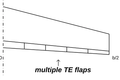
function as the twistable wing. A simple sketch of a wing with the multiple TE

flaps is shown in the Fig 1.2. These TE flaps are controllable individually just like

a bird adjusts the spanwise twist on the wing to generate the ideal distribution.

↑

multiple TE flaps

b/2 0

Figure 1.2: Schematic representation of the multiple trailing-edge flaps (right side shown).

The adaptive wing can be used not only for producing the optimum lift

distri-bution, but also for aircraft control. Azuma18studied the flight dynamics of flying

creatures and described the control with the use of adaptive wing. They trim the

body not by having horizontal and vertical tails, but adjusting the spanwise twist

on the wing. Recent research17 _{proved that this was possible with the multiple}

TE flaps if they were placed on a swept flying wing. However, this research was

only for a longitudinal control. The current research work explores the use of

multiple TE flaps for roll control. Traditionally, the rolling moment is generated

(17)

with reduced induced drag. The current work is a first step in exploring the use

of distributed controls (TE flaps) for aircraft control.

In addition, the current work also explores the use of TE flaps for generating

rolling moment on a tailless aircraft, where the TE flaps have to also satisfy a

pitching moment constraint. With continued interest in tailless aircraft such as

the Blended-wing body (BWB) concept (Fig 1.3), it is worthwhile to explore the

efficient use of distributed controls on such configurations. Finally, one of the

benefits of using distributed controls is in the redundancy they provide in case

of failure of one or more components. Towards understanding this capability, the

current study also explores the efficient use of the distributed controls in the event

of a failure of one of the TE flaps.

(18)

1.2 Outline of Thesis

This chapter has described a brief history of how the current research topic has

evolved from the previous studies. Also the motivation for conducting the current

research with the multiple TE flaps has been presented.

Moving forward, Chapter 2 describes the background information and

method-ology utilized in this research. First presented is the background information

re-lating to achievement of minimum induced and profile drag, as well as the concept

of additional and basic lift distributions and their superposition. Next section is

a derivation of the rolling moment equation for the multiple TE flaps, followed by

a brief description of the pitching moment constraint.

In the procedure section, minimization of induced drag without constraints is

first described. Then a single constraint of the rolling moment is described. In

the following section, the double constraints of the roll and pitch is presented.

Finally, for a case of the stuck flap, the equation is solved for the deflection angles

of the controllable flaps.

Results using the methodology are presented in Chapter 3 for several example

geometries. The first case is the single constraint of rolling moment. The lift

distributions are obtained for two types of wing and airfoil for different values of

the desired rolling moment. Then the results are shown for the double constraints

of roll and pitch for swept wings. Lastly, the lift distributions for the stuck flap

case on a straight wing are presented and discussed.

Chapter 4 presents brief conclusion of the research as well as some suggested

(19)

Chapter 2 Methodology

2.1 Background

In this section, background information is presented on well-known elements of

applied mathematics and aerodynamics that are used in the development of the

current method. Subsection 2.1.1 describes the theory of the relative extrema of

multi-variable functions with and without constraints. Subsection 2.1.2 describes

the derivation of the optimum flap angles for the rolling moment. Subsection 2.1.3

presents a brief review of the concept of basic and additional lift distributions.

Subsection 2.1.4 presents the induced drag of superposed lift distributions based

on Munk’s theorems. Lastly, Subsection 2.1.5 reviews the formulation of pitching

moment due to the multiple TE flaps.

2.1.1 Relative Extrema of Multi-Variable Functions with

and without Constraints

This subsection presents a mathematical technique for solving the minimum value

of a multi-variable function with and without constraints, which is discussed in

more detail in textbooks such as by Bryson and Ho.19 _{Consider a function,}_f₍_x_i),

(20)

derivative of the function with respect to every variable be zero, as follows:

∂f

∂xi

= 0 (2.1)

In addition, the sufficient condition for a minimum of f is that the Hessian

matrix, formed by elements _∂x∂2f

i∂xj be positive definite.

For a case with equality constraints given by gj(xi) = 0, the problem is solved

by modifying the objective function using unknown Lagrange multipliers, λj, as

follows:

H =f(xi) +

K

X

j=1

λjgj(xi) (2.2)

The relative extremum is found by setting the partial derivatives of H with

respect to xi and λj to be zero, as follows

∂H

∂xi

= 0 (2.3)

∂H

∂λj

= 0 (2.4)

2.1.2 Rolling Moment and Optimum Lift Distribution

The rolling moment is generated due to a different amount of total lift force

pro-duced between right and left sides of the wing. To analyze this moment explicitly,

first of all, the total lift force is derived using an element of the loading, dL.

Then the rolling moment due to the element of lift is calculated. This is shown in

Fig 2.1.

According to the definition in this figure, the rolling moment due to dL is

(21)

R (+)

dL

dy y

y

z

Figure 2.1: Rolling moment due todL (rear view).

dR = (₋dL)_·y (2.5)

The total rolling moment of an aircraft is obtained by integrating this element

of rolling moment for a whole span.

R=₋

Z b₂ −b

2 1

2ρV

2

∞

cClydy (2.6)

It is then non-dimensionalized and re-written as Eqn 2.7.

CR =−

1

Srefbref

Z b 2 −b

2

cClydy =−

2

Srefbref

Z b 2 −b

2

Γ

V∞

ydy (2.7)

This is the equation of the rolling moment coefficient, which is calculated from

the spanwise lift distribution. The equation is reformed further more to apply for

the multiple TE flaps in the Sec. 2.2.

In the remainder of this subsection, the theoretical optimum for spanwise

(22)

constraint is presented. For this derivation of the optimum lift distribution, the

standard solution procedure for lifting line theory is used. As described in several

textbooks such as Anderson,20 _{a coordinate transformation from} _y _to _θ _{is used:}

y=₋b

2cosθ (2.8)

The spanwise distribution of bound circulation, Γ(y), is expressed in as a

Fourier series in θ as usingN terms as:

Γ(θ) = 2bV∞

N

X

n=1

Ansin(nθ) (2.9)

For this representation, it can be shown that the lift coefficientCL, the induced

drag coefficientCDi and rolling moment coefficient CR can be written in terms of

the Fourier coefficients as:

CL=A1π

b2

S (2.10)

CDi =π(AR)A

2 1

1 + N

X

2

n

A

n

A1

2

(2.11)

CR =A2

πb2

4S (2.12)

It follows, therefore, that for minimumCDi at a specified CL, all Fourier terms

A2, A3, and higher are zero and the optimum lift distribution is

Γ(θ) = 2bV∞A₁sinθ = 2bV∞

C

LS

πb2

sinθ (2.13)

(23)

Γ(y) = Γ0

s

1₋

2_y

b

2

(2.14)

and the corresponding CDi is

CDi =

CL2

πAR (2.15)

When the rolling moment coefficient, CR, is also specified, the solution for

minimum CDi is satisfied by all Fourier terms A3, A4 and higher getting set to

zero. The resulting lift distribution is

Γ(θ) = 2bV∞

A1sinθ+A2sin(2θ)

= 2bV∞

CL

S

πb2sinθ+CR

4S

πb2 sin(2θ)

(2.16)

and the corresponding CDi is

CDi =

1 πAR

CL2+ 32CR2

(2.17)

2.1.3 Basic and Additional Lift Distributions

As it shown in the previous chapter, several ideas were studied to achieve a

desir-able lift distribution along the wing span. Some use geometric and aerodynamic

twist distributions and flap deflections.

The lift distribution is also affected by angle of attack, spanwise chord

distri-bution (taper), and wing sweep. The net distridistri-bution is determined by all of these

factors. Therefore, the distribution needs to be decomposed so that it can be

an-alyzed from different aspects. This is why the concept of basic and additional lift

distributions, discussed in Kuethe and Chow,21_{is very useful. As per this concept,}

(24)

and additional distributions as follows:

Cl(y) =Clb(y) +Cla(y) (2.18)

b/2 0

C la C_lb

C

l = Cla + Clb

Figure 2.2: Basic and additional lift distributions.

The basic distribution is defined at wing CL=0, and it is determined by the

geometric and aerodynamic twist, the flap deflection, and a change of airfoil or

its camber along span.

Clb =Clb,twist+Clb,camber+Clb,f lap (2.19)

The additional distribution, on the other hand, is the distribution when there

is no twist or flap deflection on the wing. It is also determined by wingCL, which

is a linear function of angle of attack if attached flow on the wing is assumed.

For this case, the wing CL is set to unity to obtain the Cla,1, then a desired CL is

substituted to calculate the additional distribution, as follows:

Cla =CLCla,1 (2.20)

(25)

are affected by the wing planform which are taper and sweep of the wing. The

concept of this superposition of these distributions is shown in Fig 2.2.

2.1.4 Induced Drag of Superposed Lift Distribution

It is well-known in wing aerodynamics that induced drag can be calculated through

the superposition of the lift distribution. Eqn 2.21 shows how the induced drag

is determined for a planar wing from the bound vorticity distribution, Γ(y), and

the associated Trefftz-plane downwash, w(y).

Dinduced =

ρ 2

Z b 2 −b

2

Γ(y)w(y)dy (2.21)

Using a small angle assumption, the Trefftz-plane induced angle of attack can

be written as:

αi(y) = w

V∞

(y) (2.22)

From Kutta-Joukowski theorem, the lift force is expressed with the circulation,

which is shown in Eqn 2.23 or non-dimensionalized of Eqn 2.24.

L′

(y0) = ρV∞Γ(y₀) (2.23)

Γ

V∞

(y) = cCl(y)

2 (2.24)

The induced drag coefficient is expressed and shown as Eqn. 2.25 based on

Eqn 2.22 and Eqn 2.24.

CDi =

1 S

Z ₂b −b

2

(26)

The lift coefficient is also derived in the following Eqn 2.26 by the

Kutta-Joukowski theorem.

CL =

1 S

Z ₂b −b

2

cCl(y)dy = 2

V∞S

Z b₂ −b

2

Γ(y)dy (2.26)

Several theories of the induced drag were derived by Max Munk22 _{and one of}

them states that the induced drag can be determined by adding the contributions

from the interaction of the elementary lift distributions and their corresponding

downwash distributions. Consider a wing with N TE flaps. Let the total lift

distribution be expressed as a superposition of the additional lift andN basic lift

distributions corresponding to the N flaps. With this approach, total induced

drag for that system can be written in terms of the contributions as follows:

Di =Daa +

N

X

i=1

(Dai+Dia) +

N

X

j=1 N

X

i=1

Dij (2.27)

Munk’s mutual drag theorem23 _{aids to simplify such expression by saying that}

the drag induced by element 1 on element 2 is equal to the drag induced by element

2 on element 1. Therefore, D12 =D21 and so on for all other elements. Also each

of these induced drag is non-dimensionalized based on the following equations.

Daa

q∞S

= CL

2

2S

Z b 2 −b

2

cCla(y)αia(y)dy =CL

2_C

Daa (2.28)

Dai

q∞S

= CL

2S

Z b 2 −b

2

cCla(y)αii(y)dyδi =CLCDaiδi (2.29)

Dij

q∞S

= 1

2S

Z b₂ −b

2

cCli(y)αij(y)dyδiδj =CDijδiδj (2.30)

Finally, the induced drag due to the N multiple TE flaps can be written as

(27)

CDi =CL

2_C

Daa+CD11δ1

2₊

· · ·+CDN NδN

2

+2CLCDa1δ1+· · ·+ 2CLCDaNδN + 2CD12δ1δ2 +· · ·+ 2CD1Nδ1δN

+2CD23δ2δ3+· · ·+ 2CD2Nδ2δN +· · ·+ 2CD(N−1)Nδ(N−1)δN

(2.31)

2.1.5 Pitching Moment with Multiple TE Flaps

Recent work by Cusher and Gopalarathnam17 _{has explored the use multiple TE}

flaps on tailless aircraft; where the pitching moment about the center of gravity

(CG) is constrained to be zero for pitch trim. This section presents some important

methods from that research.

Figure 2.3 shows the forces and moments applied to the reference section of

the wing. The moment at CG is affected by a moment occurs at the aerodynamic

center of a wing (neutral point: NP), and another moment due to an aerodynamic

lift force on the wing. This is shown in Eqn 2.32 where (Xac−_X_cg₎

¯

c is commonly

known as the static margin. It is noted that the value of the Cmacw will depend

on the wing flap angles.

Cmcg =Cmacw −CL

(Xac−Xcg)

¯

c (2.32)

For the longitudinal trim of an airplane, the moment about the center of

gravity (CG) needs to be zero (Cmcg = 0), so that the equation can be rewritten

as follows:

Cmacw =CL

(Xac−Xcg)

¯

c (2.33)

Therefore, if the static margin and a desiredCLof an aircraft are known, then

the required CMacw can be calculated by this formula.

(28)

cen-C

ref

x

ac

x

CG

W L

M

CG Mac

Figure 2.3: Forces applied to the reference section representing the relationship between pitching moments and SM.

ter of an aft-swept wing is shown in Eq. 2.34.

CMacw =

1

Sc¯

( Z b

2

−b

2

Cmac(y)c(y)

2_dy₊Z

b

2

−b

2

Clb(y)[Xac,wing−Xac(y)]c(y)dy

)

(2.34)

This equation simply explains that the total pitching moment of a wing at

the aerodynamic center is computed by summing two wing spanwise integrals of

(1) sectional pitching moment effect and (2) basic lift distribution multiplied by

its moment arm based on the wing aerodynamic center. For clarity, part (1) of

Eq. 2.34 is referred to as CMacw

sections, and (2) is referred to as

CMacw

basic.

Then the equation is simply rewritten as indicated by Eq. 2.35.

CMac,w =

CMacw

sections+

CMacw

basic =CL

(Xac−Xcg)

¯

c (2.35)

Each term CMacw

sections and

CMacw

(29)

effects based on airfoil and wing properties. They are shown in the following

equations.

CMacw

sections =

2

Sc¯

 



R

b

2

0 Cmac(y)c(y)

2_dy₊

Ry1

0 Cm_δf

1c(y)

2_dy_δ

f1 +...+

Ry_N

y_N

−1

Cm_δf

N

c(y)2_dy_δ

fN

 



(2.36)

CMacw

basic=

2

S¯c

         

        

R

b

2

0 Clb,twist(Xac,w−Xac(y))c(y)dy

+R

b

2

0 Clb,camber(Xac,w−Xac(y))c(y)dy

+

Rb₂

0 Clb,δf₁(Xac,w−Xac(y))c(y)dy

δf1 +...

+

R

b

2

0 Clb,δf_N(Xac,w−Xac(y))c(y)dy

δfN

         

        

(2.37)

Previous adaptive wing studies16 _{have shown that it is convenient to define}

the adaptive flap deflections of _{δf} be the sum of two parts: (1) the mean flap

angle, ¯δf, which is constant along span,, and (2) the variation about the mean,

n

ˆ

δf

o

. Therefore, the adaptive flap deflection angle is a summation of these two,

as shown in Eq. 2.38.

{δf}= ¯δf +

n

ˆ

δf

o

(2.38)

Then the mean flap deflection is computed by the following equation for

en-abling operation of the wing in the low-drag range of the airfoil for low profile

drag.

¯

δf =

CL−CLideal

2 sinθf

(2.39)

where θf is the angular coordinate for the hinge location x_cf in radians as

(30)

θf = cos

−1

1₋2xf

c

(2.40)

One of the biggest strength in his research was to decompose these two

equa-tions in terms of the mean flap angle and the variation angle. In order to do that,

the terms due to the variation flap in the CMacw

sections needs to be zero, which

is shown as follows:

2

S¯c

Z y1

0 Cmδfˆ1

c(y)2dy

ˆ

δf1 +...+

2

S¯c

Z y_N

y_N

−1

Cmˆ_δf

N

c(y)2dy

!

ˆ

δfN = 0 (2.41)

This is called “weighting factor (WF) equation” which is solved when a

calcu-lation of the TE flap deflection angles is achieved. The details of the WF equation

are provided in the next subsection.

Based on these methods, final forms of the Eqn 2.36 and Eqn 2.37 are shown

as follows.

CMacw

sections=

2

S¯c{

R

b

2

0 Cmac(y)c(y)

2_dy₊R

b

2

0 Cm_δf¯ c(y)2dy

¯

δf } (2.42)

CMacw

basic =

2

S¯c

 



R

b

2

0 Clb,δˆf₁(Xac,w−Xac(y))c(y)dy

ˆ

δf1 +...+

Rb₂

0 Clb,δˆf_N(Xac,w−Xac(y))c(y)dy

ˆ

δfN

 



(2.43)

2.2 Procedure

The focus of the current problem is to solve for the optimal flap distribution

(31)

according to the constraints setup, and solution procedures for each case are shown

in the following subsections.

In the first subsection, a solution of the multiple TE flap deflection equation

without constraints is described. Second part presents a calculation with a rolling

moment control, which is a single constraint. Then the computation with multiple

constraint is described. The last section describes the stuck-flap analysis and its

calculation, which is the adaptive flap deflection computation when one of the

flaps is stuck at some deflection angle.

2.2.1 Minimization of Induced Drag without Constraints

According to the requirements of the relative extrema in subsection 2.1.1, the first

partial derivatives of the Eqn 2.31 were computed for variation flap angles, and

set to zero as shown in the Eqn 2.44.

     

    

∂C_Di

∂δˆ1 = 2CLCDa1 + 2CD11

ˆ

δ1+ 2CD12ˆδ2+· · ·+ 2CD1NδˆN = 0

... ∂C_Di

∂ˆδN = 2CLCDaN + 2CDN N

ˆ

δN + 2CD1Nδˆ1+· · ·+ 2CD(N−1)N

ˆ

δN−₁ = 0

     

    

(2.44)

These equations are simplified and rewritten in a matrix form as follows:



        

2CD11 2CD12 · · · 2CD1N

2CD21 · · · ...

... . .. ...

2CDN1 · · · 2CDN N



        

         

        

ˆ

δ1

ˆ

δ2

... ˆ

δN

         

        

=

         

        

−2CLCDa1

−2CLCDa2

...

−2CLCDaN

         

        

(2.45)

A square matrix with drag coefficients in the left hand side of the equation is

referred to here as the “drag matrix”. It is necessary to mention here that the

(32)

with the matrix equation as shown. This is why the weighting factor equation is

applied to this to obtain the unique solution of the flap deflections.

The wingCLin the right hand side of the equation is the desired lift coefficient.

A vector with flap deflections is the output of the system which is the adaptive

flap deflections. Since the drag matrix and the right hand side vector can be

computed, the final goal of the flap deflections is obtained after applying the

weighting factor.

The weighting factor equation for the rolling moment constraint is now

pre-sented. Assuming that the flap to chord ratio being constants, the Eqn. 2.46 can

be derived for non-constant chord distributions and different flap spans.

¯

δf = ˆδ1·

S1

Sref

+ ˆδ2·

S2

Sref

+_{· · ·}+ ˆδN ·

SN

Sref

= CL−CLideal

2sinθf

(2.46)

Now this weighting factor equation is applied to the system.



        

2CD11 · · · 2CD1N

... . .. ...

2CDN1 · · · 2CDN N

( S1

Sref) · · · (

SN

Sref)



        

     

    

ˆ

δ1

... ˆ

δN

     

    

=

         

        

−2CLCDa1

...

−2CLCDaN

¯

δf

         

        

(2.47)

It is convenient to use a Vortex Lattice Method (VLM) or a panel method

for computing the elements of the drag matrix and the RHS. For this research, a

code called AVL (Athena Vortex Lattice)24 _{is used. Using the AVL, first of all, the}

additional case was run and the lift and downwash distributions were obtained.

Then all basic cases with each flap deflections were computed.

Because of the use of AVL, the drag matrix with the drag coefficients as well

as ones in the right hand side can be computed based on Eqn 2.28, Eqn 2.29,

(33)

2.2.2 Minimization of Induced Drag with Rolling

Moment Constraint

In order to utilize Eqn 2.7 for the adaptive wing with the basic and additional

loading theory, the Eqn 2.18 is applied as shown below.

CR=−

1

Srefbref{

Z ₂b −b

2

cClbydy+

Z b₂ −b

2

cCLCla,1ydy} (2.48)

The additional distribution is a lift distribution with zero flap deflections and

zero spanwise twist on the wing. This means that the distribution is symmetric on

both sides of the wing. Therefore, the additional distribution has no contribution

to a production of the rolling moment. Also, this research focuses on the TE flaps

but not any twist or camber change along the span based on Eqn 2.19. Therefore

the Eqn 2.48 is rewritten as follows.

CR =−

1

Srefbref{

Z b₂ −b

2

cClb,f lapydy} (2.49)

1 2 ... ... (N−1) N

Figure 2.4: Adaptive flaps (top view).

Throughout this research the multiple TE flaps are numbered as shown in

Figure 2.4 which is numbered for the whole span. According to this setup, the

(34)

CR=− 1

Srefbref{

(

Z b₂ −b

2

cClb,δ1ydy)δ1+· · ·+ ( Z ₂b

−b 2

cClb,δNydy)δN} (2.50)

According to Eqn 2.38, the flap deflection is decomposed as mean and

vari-ation terms. Also, the mean is constant along span and therefore, it does not

have a contribution in generating the rolling moment. Therefore, the equation is

rewritten as follows.

CR=−

1

Srefbref{

(

Z b 2 −b

2

cC_lb,ˆ_δ₁ydy)ˆδ1+· · ·+ (

Z b 2 −b

2

cC_lb,ˆ_δ_Nydy)ˆδN} (2.51)

The Eqn 2.51 is a final expression of the rolling moment equation due to the

multiple TE flaps. This equation is then used to as a constraint of the system of

the multiple TE flaps. The mean flap angle, which was explained in the previous

section, is a function of the weighting factor which shows the relative effectiveness

of each flaps.

Using the method of Lagrange multipliers (λ), as explained in Bryson and

Ho,19 _{the constraint equation,}_g_{, is the rolling moment equation of Eqn 2.51.}

g(xi) = (CR)desired+ 1

Srefbref{

(

Z b 2 −b

2

cC_lb,ˆ_δ₁ydy)ˆδ1+· · ·+ (

Z b 2 −b

2

cC_lb,_δˆ_Nydy)ˆδN}= 0

(2.52)

Finally, this method of Lagrange multipliers for the constraint is applied to

(35)

             

2CD11 · · · 2CD1N

1 Sb R b 2 −b 2 cC_l

b,δˆ1ydy

... . .. ... ...

2CDN1 · · · 2CDN N

b,δˆNydy

( S1

Sref) · · · (

SN

Sref) 0

−Sb1

R b 2 −b 2 cC_l

b,ˆδ1ydy · · · −

b,ˆδNydy 0

                                 ˆ δ1 ... ˆ δN λ                    =                           

−2CLCDa1

...

−2CLCDaN

¯

δf

(CR)desired

                           (2.53)

This is the final expression of the matrix equation with constraint. Then each

of the system with and without the constraints (Eqn 2.47, Eqn 2.53) are solved

for various wing configurations. Those results are shown in the next chapter.

2.2.3 Minimization of Induced Drag with Pitch and Roll

Constraints

In this section, the equations for dual constraints on rolling and pitching moment

are presented. The weighting factor equation is adapted from the work of Cusher

and Gopalarathnam.17 _{Just like the rolling moment constraint, the weighting}

(36)

         

2CD11 . . . 2CD1N

... . .. ...

2CDN1 . . . 2CDN N

2 S¯c

Ry1

0 Cmˆ_δf 1

c(y)2_dy _{. . .} 2

S¯c

RyN

yN−1Cmδfˆ

N

c(y)2_dy

                     ˆ δ1 ... ˆ δN            =                   

−2CLCDa1

...

−2CLCDaN

0                    (2.54)

This is a system without constraints from pitching moment standpoint. This

system will provide a very similar output with the one by Eqn 2.47.

The system with a single constraint of pitching moment is determined based

on Eqn 2.2 and Eqn 2.43.

             

2CD11 . . . 2CD1N −

2 Sc¯

R

b

2

0 Clb,ˆδf₁∆xcdy

... . .. ... ...

2CDN1 . . . 2CDN N −

2 Sc¯

R₂b

0 Clb,ˆδ_fN∆xcdy 2

S¯c

Ry₁

0 Cm_δfˆ 1

c2dy . . . _S2_¯_cRyN

yN−1Cmδfˆ

N

c2dy 0

2 S¯c

R

b

2

0 Clb,ˆδf₁∆xcdy . . .

2 S¯c

R

b

2

0 Clb,δˆ_fN∆xcdy 0

                                 ˆ δ1 ... ˆ δN λ                    =                           

−2CLCDa1

...

−2CLCDaN

0

CMacw

basic                            (2.55)

In the equation, ∆x represents the term Xac,w−Xac(y). There are two ways

of computing its output based on cases of reducing the induced drag only and the

one with profile drag. Cusher referred to these as Scheme A and Scheme B.

First of all, the static margin of an aircraft is set as well as a desired wing CL.

Then the wing pitching moment is determined by Eqn 2.33.

(37)

substituted into the Eqn 2.43 to obtain (CMacw)basic. Then the (CMacw)sections can

be computed by Eqn 2.35. Finally the mean flap angle is found by Eqn 2.42 to

obtain the final flap deflection angles by Eqn 2.38.

For the Scheme B, the CLideal is determined due to the airfoil selection. From

the obtained mean flap angle, the (CMacw)sections is computed by the Eqn 2.42.

This enables to calculate (CMacw)basicby Eqn 2.35. Finally the system of Eqn 2.55

is computed to obtain the total flap deflections of _{δf}.

Since the single constraint of rolling moment has been applied to the system

as well as the pitching moment, two constraint of pitch and roll are applied to

the system so that it compute the adaptive flap deflections based on these two

constraints.

The multiple constraints are achieved based on the Eqn 2.2. To able to obtain

output for SchemeAandBof the pitching moment constraint, the rolling moment

(38)

             

2CD11 . . . 2CD1N R1

... . .. ... ...

2CDN1 . . . 2CDN N RN

2 S¯c

Ry1

0 Cm_δfˆ 1

c2_dy _{. . .} 2

Sc¯

RyN

yN−1Cmˆδf

N

c2_dy ₀

−R1 · · · −RN 0

              ·                    ˆ δ1 ... ˆ δN λ1                    =                           

−2CLCDa1

...

−2CLCDaN

0

(CR)_basic

                           (2.56)                  

2CD11 . . . 2CD1N R1 −P1

... . .. ... ... ...

2CDN1 . . . 2CDN N RN −PN

2 Sc¯

Ry1

0 Cmˆ_δf 1

c2_dy _{. . .} 2

S¯c

RyN

yN−1Cmδfˆ

N

c2_dy ₀ ₀

−R1 · · · −RN 0 0

P1 . . . PN 0 0

                  ·                            ˆ δ1 ... ˆ δN λ1 λ2                            =                                   

−2CLCDa1

...

−2CLCDaN

0

(CR)_basic

CMacw

basic                                    (2.57)

In which Rn = _Sb1

Rb₂ −b

2

cC_l

b,δˆnydy, and Pn = −

2 Sc¯

R₂b

0 Clb,δˆ_fn∆xcdy for equation

(39)

These two equations are used for each scheme according to the previous

sec-tions of Sec 2.2.2 with the rolling moment requirement from Sec 2.1.2.

2.2.4 Optimum Loading with a Control Failure

The system matrix can also be solved when one of the flaps is stuck at a known

angle due to control failure. For this research only a single constraint of rolling

moment is considered.

First of all, the stuck flap was chosen as the xth which is between 1st andNth

in the total number ofN TE flaps. Noting that ∂CDi

∂δˆx is not set to zero, the system

matrix of Eqn 2.47 is modified as follows.

2CD11(ˆδ1) +· · ·+ 2CD1x(ˆδx) +· · ·+ 2CD1N(ˆδN) = −2CLCDa1

...

2CD(x−1)1(ˆδ1) +· · ·+ 2CD(x−1)x(ˆδx) +· · ·+ 2CD(x−1)N(ˆδN) =−2CLCDa(x−1)

2CD(x+1)1(ˆδ1) +· · ·+ 2CD(x+1)x(ˆδx) +· · ·+ 2CD(x+1)N(ˆδN) = −2CLCDa(x+1)

...

2CDN1(ˆδ1) +· · ·+ 2CDN x(ˆδx) +· · ·+ 2CDN N(ˆδN) = −2CLCDaN

S1

Sref(ˆδ1) +· · ·+

Sx

Sref(ˆδx) +· · ·+

SN

Sref(ˆδN) = ¯δf

(2.58)

Since the ( ˆδx) is known, all the terms including this are moved to the right

(40)

2CD11(ˆδ1) +· · ·+ 2CD1N(ˆδN) = −2CLCDa1−2CD1x(ˆδx)

...

2CD(x−1)1(ˆδ1) +· · ·+ 2CD(x−1)N(ˆδN) = −2CLCDa(x−1)−2CD(x−1)x(ˆδx)

2CD(x+1)1(ˆδ1) +· · ·+ 2CD(x+1)N(ˆδN) = −2CLCDa(x+1) −2CD(x+1)x(ˆδx)

...

2CDN1(ˆδ1) +· · ·+ 2CDN N(ˆδN) = −2CLCDaN −2CDN x(ˆδx)

S1

Sref(ˆδ1) +· · ·+

SN

Sref(ˆδN) = ¯δf −

Sx

Sref(ˆδx)

(2.59)

These equations are now reshaped as the matrix form as follows.

                     

2CD11 · · · 2CD1x−1 2CD1x+1 · · · 2CD1N

... _{· · ·} ... ... _{· · ·} ...

2CD(x−1)1 · · · 2CD(x−1)x−1 2CD(x−1)x+1 · · · 2CD(x−1)N

2CD(x+1)1 · · · 2CD(x+1)x−1 2CD(x+1)x+1 · · · 2CD(x+1)N

... _{· · ·} ... ... _{· · ·} ...

2CDN1 · · · 2CDN x−1 2CDN x+1 · · · 2CDN N

( S1

Sref) · · · (

Sx−1

Sref) (

Sx+1

Sref) · · · (

SN

Sref)

                                                         ˆ δ1 ... ˆ

δx−₁

ˆ

δx+1

... ˆ δN                                    =                                           

−2CLCDa1 −2CD1x(ˆδx)

...

−2CLCDa(x−1)−2CD(x−1)x(ˆδx)

−2CLCDa(x+1) −2CD(x+1)x(ˆδx)

...

−2CLCDaN −2CDN x(ˆδx)

¯

δf −_SS_refx (ˆδx)

                                           (2.60)

The size of the LHS matrix is (N)_×(N₋1), the output deflection vector size

(41)

solved.

For a case with a rolling moment control, the constraint equation is simply

added to this newly organized matrix as follows. In the equation Rn represents

the term _Sb1 R

b

2 −b

2

cC_l_b_,_δˆ_nydy.

                         

2CD11 · · · 2CD1x−1 2CD1x+1 · · · 2CD1N R1

... _{· · ·} ... ... _{· · ·} ... ...

2CD(x−1)1 · · · 2CD(x−1)x−1 2CD(x−1)x+1 · · · 2CD(x−1)N Rx+1

2CD(x+1)1 · · · 2CD(x+1)x−1 2CD(x+1)x+1 · · · 2CD(x+1)N Rx−1

... _{· · ·} ... ... _{· · ·} ... ...

2CDN1 · · · 2CDN x−1 2CDN x+1 · · · 2CDN N RN

( S1

Sref) · · · (

Sx−1

Sref) (

Sx+1

Sref) · · · (

SN

Sref) 0

−R1 · · · −Rx−₁ −R_x₊₁ · · · −R_N 0                                                                      ˆ δ1 ... ˆ

δx−1

ˆ

δx+1

... ˆ δN λ                                            =                                                   

−2CLCDa1 −2CD1x(ˆδx)

...

−2CLCDa(x−1)−2CD(x−1)x(ˆδx)

−2CLCDa(x+1) −2CD(x+1)x(ˆδx)

...

−2CLCDaN −2CDN x(ˆδx)

¯

δf −_SS_refx (ˆδx)

(CR)_basic+Rx

                                                   (2.61)

Therefore, all the elements of the drag matrix are known as well as the elements

of the right hand side vector. This system can then be solved for the controllable

TE flap deflection angles.

If the number of stuck flaps are more than two, then the system matrix can

also be solved following the same steps with two known TE deflection angles. For

(42)

Chapter 3 Results

In this chapter, results for different test cases are presented and discussed. To

obtain the results, a few example wings are used, with dimensions and airfoil

selections shown in the Section 3.1.

Section 3.2 shows the results with a single constraint of rolling moment.

Sec-tion 3.3 shows the results for two constraints of rolling and pitching moments.

Section 3.4 shows some results for a single constraint of the rolling moment with

a stuck flap as an example of control failure.

3.1 Test Cases

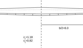
Three kinds of wing shapes are used as examples for this research. The first

wing is a straight-tapered wing with the taper-ratio (λ) of 0.7, shown in Fig. 3.1.

This wing was used for a case of single constraint of rolling moment. The next

two wings are the swept-tapered-wing with the sweep (Λc/4) of 20 degrees and 35

degrees with the same taper-ratio, shown in Fig. 3.2. These two wings were used

for both single and multiple constraint cases.

Using these two wings, a hypothetical tailless aircraft was used as an sample

platform with characteristics displayed in Table 3.1. These characteristics were

(43)

Table 3.1: Assumed parameter values for example tailless aircraft.

Static Parameters Value

Gross weight (W) 14,200 N

(3,200 lbf)

Mean aerodynamic chord (¯c) 1.01 m

(3.31 ft)

Reference area (S) 12.0 m2

(130 ft2₎

Wing aspect ratio (AR) 12

Static margin (SM) 10 % ¯c

Number of half-span TE flaps (N) 5

Flap-to-chord ratio (all flaps) 0.2

Variable Parameters Value

1

4 chord sweep angle (Λc/4) 20 deg

35 deg

Airfoil section NLF0824 (CAM BERED)

(Cm0 =−0.0802)

Reflex055 (REF LEXED)

(Cm0 = 0.055)

For each wing shape, two different airfoils were used which were the same

airfoils used in Ref. 17. The first airfoil is a cambered NLF airfoil which has a zero

lift pitching moment coefficient (Cm0) of −0.0802, and is labeled CAM BERED.

This airfoil has a well defined low drag range. The second airfoil is a reflexed

airfoil which was designed to have a positive Cm0 value of 0.055, and is named

REF LEXED. Figures 3.3 and 3.4 display the properties of these airfoils as

analyzed by XFOIL25 _{calculated at a} _Re√_C

l of three million, as well as their

corresponding geometries.

Based on these wing and airfoil selections, there are four example cases for

a single constraint and four cases for multiple constraints case. Example Case

#1₋1 is the CAM BERED airfoil for a straight-tapered wing. Example Case

#1₋2 is the CAM BERED airfoil at Λc/4 = 35 deg of wing sweep. Example

(44)

b/2=6.0

c

r=1.18

c

t=0.82

Figure 3.1: Example planform for unswept tapered wing with 5 TE flaps per half span.

Λ_c/4=20°

b/2=6.0 c

r=1.18

c

t=0.82

(a)

Λ_c/4=35°

b/2=6.0 c

r=1.18

c

t=0.82

(b)

Figure 3.2: Wing planform for swept tapered wing with 5 TE flaps per half span:

(a) Λc/4 of 20 degrees and (b) Λc/4 of 35 degrees.

Case #1₋4 is the REF LEXED airfoil with Λc/4 = 35 deg of sweep. For each

of these cases, the desired rolling moment coefficient values were set to CR=0.02

and CR=0.04 respectively. These desired values of CR were determined as the

rolling-moment coefficients for a generic transport aircraft with 5 deg and 10 deg

aileron deflections.

For the multiple constraint case, two examples are studied. Example Case

#2 ₋1 is the CAM BERED airfoil at Λc/4 = 35 deg. Example Case #2−2

is the REF LEXED airfoil at Λc/4 = 20 deg. Each case were applied for both

SchemeAand SchemeB which is shown in Cusher17_{with the two rolling moment}

coefficient values. For the supplemental analysis of a stuck flap in Sec. 3.4, only

the straight-tapered wing with CAM BERED airfoil is studied. However, two

flaps were chosen as the stuck flaps and each case of data was taken with zero

(45)

0 0.2 0.4 0.6 0.8 1 −1.5

−1

−0.5

0

0.5

1

x/c C_p

C_l = 0.5

(a)

0 0.001 0.002 0.003 0.004 0.005 0.006 0.007 0.008 0.009 0.01 0

0.1 0.2 0.3 0.4 0.5 0.6 0.7 0.8 0.9 1

C

d

C

l

(b)

Figure 3.3: CAM BEREDairfoil: (a) Geometry andCpdistribution and (b) drag

polar at Re√Cl of three million.

0 0.2 0.4 0.6 0.8 1 −1.5

−1

−0.5

0

0.5

1

x/c C_p

C_l = 0.5

(a)

0 0.001 0.002 0.003 0.004 0.005 0.006 0.007 0.008 0.009 0.01 0

0.1 0.2 0.3 0.4 0.5 0.6 0.7 0.8 0.9 1

C

d

C

l

(b)

Figure 3.4: REF LEXED airfoil: (a) Geometry andCp distribution and (b) drag

(46)

tip, which is called F lap.1, and another located next to the wing root on the

right hand side of the wing, which is namedF lap.6. For each case the two rolling

moment coefficient values were applied.

3.2 Rolling Moment Constraint

3.2.1 Example Case

#1

₋

1

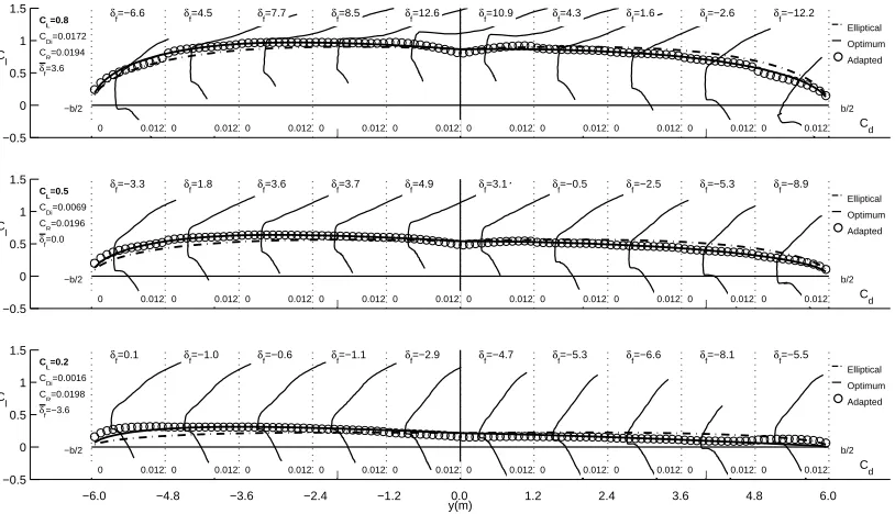
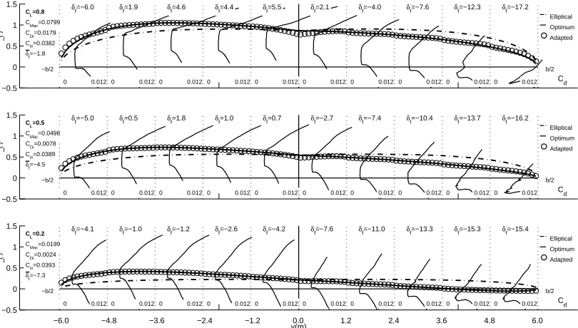
The first case is theCAM BEREDairfoil used on the straight-tapered wing

plan-form with no sweep angle shown in Fig. 3.1. The Cl distribution and drag polar

for each flap are shown in the Fig. 3.5. The desired rolling moment coefficient,

CRdesired, is 0.02. Three Cl distributions for the different wing CL values of 0.2,

0.5, 0.8 are shown in the figure. For each distribution the total induced drag,

rolling moment coefficients, and mean flap deflection angles are shown on the left

in the plot. The distribution shown as a dash-dot line is the elliptical

distribu-tion. This distribution has no rolling moment because it is symmetric about the

wing root. TheCldistribution with a solid line is the optimum distribution which

was described in Sec. 2.1.2. The distribution with circle markers is the adapted

distribution achieved by using the multiple TE flap deflections. For each flapped

portion of the wing, the drag polar for that flap angle is plotted, to check if that

portion of the wing is operating within the drag bucket of the airfoil.

It is clear that the adapted distribution is very close to the optimum serves to

verify the theory of induced drag minimization with the rolling moment constraint.

The flap angles are listed in Fig. 3.5 for each CL. It is seen the flap angles are

all moderate and not high enough for flow separation to be a concern. It is also

seen that each portion of the wing is operating within the corresponding low-drag

range, resulting in minimum profile drag in addition to minimum induced drag.

(47)

−6 −4 −2 0 2 4 6 −0.5 0 0.5 1 1.5 Elliptical Optimum Adapted b/2 −b/2

δf=0.2

0 0.012

δf=6.2

0 0.012

δf=7.2

0 0.012

δf=6.7

0 0.012

δf=5.3

0 0.012

δf=4.5

0 0.012

δf=4.2

0 0.012

δf=3.1

0 0.012

δf=0.9

0 0.012

δf=−4.9

0 0.012

CL=0.8

CDi=0.0173 CR=0.0197

δf=3.6

C_l

C

d

−6 −4 −2 0 2 4 6

−0.5 0 0.5 1 1.5 Elliptical Optimum Adapted b/2 −b/2

δf=−0.1

0 0.012

δf=2.4

0 0.012

δf=2.7

0 0.012

δf=2.1

0 0.012

δf=1.1

0 0.012

δf=0.3

0 0.012

δf=−0.3

0 0.012

δf=−1.3

0 0.012

δf=−2.9

0 0.012

δf=−5.1

0 0.012

CL=0.5

CDi=0.0069 CR=0.0198

δf=0.0

C_l

C_d

−6 −4 −2 0 2 4 6

−0.5 0 0.5 1 1.5 Elliptical Optimum Adapted b/2 −b/2 −6.0 δf=−0.4

0 0.012

−4.8 δf=−1.5

0 0.012

−3.6 δf=−1.7

0 0.012

−2.4 δf=−2.4

0 0.012

−1.2 δf=−3.1

0 0.012

0.0 δf=−3.9

0 0.012

1.2 δf=−4.9

0 0.012

2.4 δf=−5.8

0 0.012

3.6 δf=−6.7

0 0.012

4.8 δf=−5.4

0 0.012 6.0 C L=0.2 C Di=0.0015 C R=0.0199 δ f=−3.6 C l C_d y(m)

Figure 3.5: Spanwise Cl distributions with flap-section drag polars and optimal

Cl distributions with CRdesired=0.02 for Example Case #1−1.

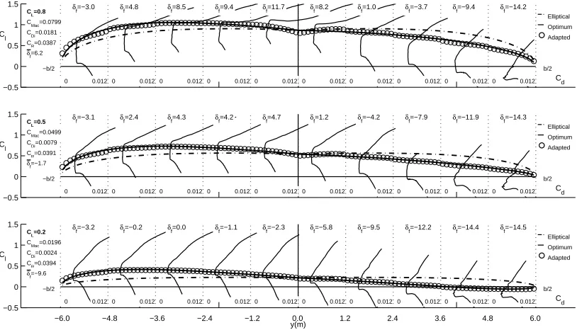
−6 −4 −2 0 2 4 6

δ_f=2.7

0 0.012

δ_f=8.8

0 0.012

δ_f=9.2

0 0.012

δ_f=7.9

0 0.012

δ_f=5.7

0 0.012

δ_f=4.1

0 0.012

δ_f=3.0

0 0.012

δ_f=1.1

0 0.012

δ_f=−1.7

0 0.012

δ_f=−7.4

0 0.012

CL=0.8

CDi=0.0182 CR=0.0394

δf=3.6

C_l

C

d

−6 −4 −2 0 2 4 6

δf=2.4

0 0.012

δf=5.0

0 0.012

δf=4.8

0 0.012

δf=3.4

0 0.012

δf=1.5

0 0.012

δf=−0.1

0 0.012

δf=−1.6

0 0.012

δf=−3.4

0 0.012

δf=−5.6

0 0.012

δf=−7.7

0 0.012

CL=0.5

CDi=0.0079 CR=0.0396

δf=0.0

C_l

C

d

−6 −4 −2 0 2 4 6

−0.5 0 0.5 1 1.5 Elliptical Optimum Adapted b/2 −b/2 −6.0 δf=2.2

0 0.012

−4.8 δf=1.2

0 0.012

−3.6 δf=0.3

0 0.012

−2.4 δf=−1.2

0 0.012

−1.2 δf=−2.7

0 0.012

0.0 δf=−4.3

0 0.012

1.2 δf=−6.1

0 0.012

2.4 δf=−7.8

0 0.012

3.6 δf=−9.4

0 0.012

4.8 δf=−7.9

0 0.012 6.0 C L=0.2 C Di=0.0025 C R=0.0397 δ f=−3.6 C l C_d y(m)

Figure 3.6: Spanwise Cl distributions with flap-section drag polars and optimal

Optimum Flap Angles for Roll Control on Wings with Multiple Trailing-Edge Flaps

ABSTRACT

Optimum Flap Angles for Roll Control on Wings with

Multiple Trailing-Edge Flaps

BIOGRAPHY

ACKNOWLEDGEMENTS

Table of Contents

List of Tables

List of Figures

Nomenclature

Chapter 1

Introduction

1.1

Background

1.2

Outline of Thesis

Chapter 2

Methodology

2.1

Background

2.1.1

Relative Extrema of Multi-Variable Functions with

and without Constraints

2.1.2

Rolling Moment and Optimum Lift Distribution

2.1.3

Basic and Additional Lift Distributions

2.1.4

Induced Drag of Superposed Lift Distribution

2.1.5

Pitching Moment with Multiple TE Flaps

2.2

Procedure

2.2.1

Minimization of Induced Drag without Constraints

2.2.2

Minimization of Induced Drag with Rolling

Moment Constraint

2.2.3

Minimization of Induced Drag with Pitch and Roll

Constraints

2.2.4

Optimum Loading with a Control Failure

Chapter 3

Results

3.1

Test Cases

3.2

Rolling Moment Constraint

3.2.1

Example Case

#1

−

1

₋