and Trajectory Reconstruction of the Orion Command Module from Scale Model Aer-oballistic Flight Data. (Under the direction of Professor Robert Tolson).
by
Thomas Sebastian
A thesis submitted to the Graduate Faculty of North Carolina State University
In partial fulfillment of the Requirements for the Degree of
Master of Science
Aerospace Engineering
Raleigh, North Carolina
2008
APPROVED BY:
_______________________________ Robert Tolson, Chair of Advisory Committee
_______________________________ ______________________________
Biography
Acknowledgments
I would like to extend my sincere thanks to Dr. Robert Tolson for serving as my adviser throughout this project. His vast experience and insight have enhanced my graduate school experience and have been a great aid in my continuing forays into the world of academia and research. His examples of professionalism, curiosity, and work ethic are qualities that I will attempt to emulate throughout the rest of my career. I would also like to thank Dr. Fred DeJarnette and Dr. Andre Mazzoleni for serving on my thesis committee and for providing useful feedback. I would also like to thank each of them for the encouragement and support they each provided in my various undergraduate research projects. Mark Schonenberger of the Atmospheric Flight & Entry Systems Branch at the NASA Langley Research Center provided me with invaluable assistance in overcoming technical and logistical hurdles encountered in the project. His advice and direction is greatly appreciated.
Finally, I want to thank my family. My wife, Catherine, has been supportive during all of my work and has always been there to oer words of encouragement when they were most needed. My brothers, Johnny and Mathew, have always been a source of inspiration to me and have been my best friends. Finally, I would like to thank my parents for their unconditional love and patience. They took the giant step of coming to America in order to provide more opportunities for their children. They have, most appreciatively, reminded me that there is more to life than diagrams and reports and that relationships are just as, if not more, important.
Table of Contents
List of Figures . . . vi
List of Tables . . . x
1 Introduction . . . 1
1.1 The Vision for Space Exploration . . . 1
1.2 Crew Exploration Vehicle . . . 2
1.3 Research Goals . . . 4
2 Experimental Methods for Obtaining Vehicle Dynamics . . . 6
2.1 Aeroballistic Range Testing . . . 7
2.2 Proving Grounds . . . 10
2.3 On-board Instrumentation . . . 11
2.3.1 CEV Telemetry Module . . . 12
2.3.2 CEV-TM Calibration . . . 14
3 Post-Flight Analysis of CEV-TM Data . . . 16
3.1 Transformations . . . 19
3.2 Determination of Aerodynamic Coecients . . . 27
4 Aeroballistic Testing with Pressure Transducers . . . 32
4.1 Pressure Transducers . . . 34
4.2 Pressure Transducer Calibration . . . 36
5 Constructing an Aerodynamic Database . . . 39
5.1 Wind Tunnel Testing . . . 39
5.2 Computational Fluid Dynamics Simulations . . . 42
5.3 Development of an Analytic Pressure Model . . . 46
5.4 Pressure Tap Placement . . . 53
6 Parameter Estimation . . . 58
6.1 Least Squares Approach . . . 58
6.2 Minimum Variance Approach with A Priori . . . 64
6.3 Method Validation . . . 68
7 Post-Flight Analysis of CEV-PTM Data . . . 81
7.1 Data Preprocessing . . . 81
7.2 Parameter Estimation Assuming No Scale Factors or Biases . . . 86
7.3 Parameter Estimation With Scale Factors and Biases . . . 95
7.4 CEV-PTM Aerodynamic Coecients . . . 106
8 Conclusions . . . 111
List of Figures
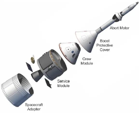
Figure 1.1 CEV stack components . . . 3
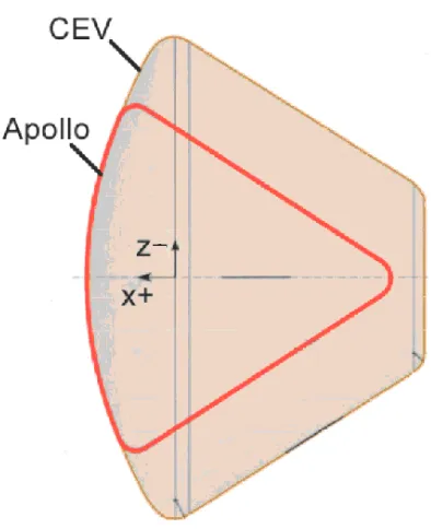
Figure 1.2 Size comparison between Orion CM and Apollo CM . . . 4
Figure 2.1 Diagram of aeroballistic range . . . 8
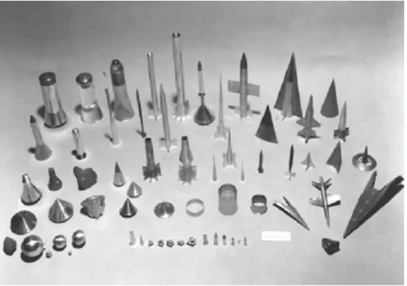
Figure 2.2 Examples of Aeroballistic Test Articles . . . 9
Figure 2.3 ARL proving grounds . . . 10
Figure 2.4 DFuze housing and circuit boards . . . 12
Figure 2.5 Cutaway image of CEV-TM . . . 13
Figure 3.1 Captured frames from high-speed tracking camera . . . 16
Figure 3.2 Filtered accelerometer output from CEV-TM-4 . . . 17
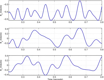
Figure 3.3 Filtered magnetometer output from CEV-TM-4 . . . 18
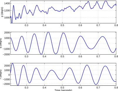
Figure 3.4 Filtered angular rate gyroscope output from CEV-TM-4 . . . 19
Figure 3.5 Rotation between range and NED coordinate systems . . . 21
Figure 3.6 Rotation between NED and magnetic eld coordinate systems . 23 Figure 3.7 Rotation between magnetic eld and body coordinate systems . 24 Figure 3.8 Comparison of normalized phase-correcting parameters . . . 26
Figure 3.9 CEV ight angles generated by minimum error solution . . . 27
Figure 3.10 CEV normal and lifting force coecients . . . 29
Figure 4.1 Diagram of CEV-PTM . . . 33
Figure 4.2 Kulite XCEL-100 pressure transducer . . . 35
Figure 4.3 CEV-PTM-01 static pressure calibration response . . . 37
Figure 4.4 Noise levels and histogram of #3 pressure tap residuals . . . 38
Figure 5.1 NASA Ames Unitary Plan Wind Tunnel . . . 40
Figure 5.2 Wind tunnel CM model with sting assembly and trip dots . . . . 41
Figure 5.3 CFD and wind tunnel test range and grid/tap locations on Orion CM forebody . . . 44
Figure 5.4 CFD and wind tunnel pressure coecient variation at cone angle of 19.45-degrees . . . 45
Figure 5.5 Comparison of series with dierent numbers of coecients . . . . 47
Figure 5.6 Percent dierence of CFD 3-term analytical model . . . 48
Figure 5.7 Quadratic relationship between angle of attack and 3-term model coecients . . . 49
Figure 5.8 Percent dierence of CFD 7-term analytical model . . . 50
Figure 5.9 Anchored analytical model compared to unanchored model and wind tunnel datapoints at cone angle of 19.45-degrees . . . . 52
Figure 5.10 Stagnation point cone angle over a range of angles of attack at varying Mach numbers . . . 55
Figure 5.11 Comparison of CFD and wind tunnel Orion CM data on vertical and horizontal planes . . . 56
Figure 6.1 POST-generated ight parameters and simulated pressure prole 69 Figure 6.2 Residuals of ltered POST-based pressure prole . . . 70
Figure 6.4 Mach number solution for 9-tap least squares solution . . . 72
Figure 6.5 Angle of attack solution for 9-tap least squares solution . . . 73
Figure 6.6 Sideslip angle solution for 9-tap least squares solution . . . 74
Figure 6.7 Pressure residuals for 9-tap minimum variance with a priori solution 75 Figure 6.8 Mach number solution for 9-tap minimum variance with a priori solution . . . 76
Figure 6.9 Angle of attack solution for 9-tap minimum variance with a priori solution . . . 77
Figure 6.10 Sideslip angle solution for 9-tap minimum variance with a priori solution . . . 78
Figure 7.1 Example of ltering output for 9-tap case, pressure tap #2 . . . 82
Figure 7.2 5 and 9-tap pressure data collected from CEV-PTM shots . . . . 83
Figure 7.3 Comparison of radar to pressure-based Mach number estimate (using isentropic and normal shock relations) . . . 85
Figure 7.4 Pressure residuals for 5-tap case . . . 87
Figure 7.5 Converged Mach plot for 5-tap case . . . 88
Figure 7.6 Flight angles for the 5-tap case . . . 89
Figure 7.7 Pressure residuals for 9-tap case . . . 90
Figure 7.8 Converged Mach plot for 9-tap case . . . 91
Figure 7.9 Flight angles for the 9-tap case . . . 92
Figure 7.13 5-tap solution for ight angles with scale factor and bias estimates 97 Figure 7.14 9-tap pressure residuals and Mach number solution with scale
factor and bias estimates . . . 98
Figure 7.15 9-tap solution for ight angles with scale factor and bias estimates 99 Figure 7.16 9-tap standard deviations for ight parameters . . . 100 Figure 7.17 Pressure residuals for 9-tap case with weighted pressure
uncer-tainties . . . 102 Figure 7.18 9-tap solution for Mach number with weighted pressure uncertainties103 Figure 7.19 9-tap solution for ight angles with weighted pressure uncertainties104 Figure 7.20 9-tap standard deviations for ight parameters with weighted
List of Tables
Table 3.1 Comparison of coecients between analytical method and
EX-TRACTR . . . 30
Table 6.1 A priori uncertainties set for solution parameters . . . 74
Table 6.2 Mean and standard deviation of estimated parameter residuals
using least squares and minimum variance with a priori . . . 78
Table 6.3 Mean and standard deviation of pressure residuals using least
squares and minimum variance with a priori . . . 79
Table 6.4 Comparison of converged scale factors and biases using least squares
and minimum variance with a priori . . . 79
Table 7.1 Uncertainty of pressure transducers . . . 101
Table 7.2 9-tap scale factors and biases with weighted pressure uncertainties 106
Chapter 1
Introduction
1.1 The Vision for Space Exploration
In the aftermath of STS-107, the National Aeronautics and Space Administration (NASA) was tasked to pursue a new human exploration agenda. This new framework, the Vision for Space Exploration (VSE), was released to the public in February 2004. The fundamental goal of the VSE is to advance U.S. scientic, security, and economic interests through a robust and sustainable space exploration program. The following objectives were proposed to meet this goal [1]:
Implement a sustained and aordable human and robotic program to explore the solar system and beyond
Extend human presence across the solar system, starting with a human return to the Moon by the year 2020, in preparation for human exploration of Mars and other destinations
and to support decisions about the destinations for human exploration
Promote international and commercial participation in exploration to further U.S scientic, security, and economic interests
The Space Shuttle has been the workhorse of the U.S. manned space exploration pro-gram. The eet has conducted operations since 1981, transporting crews to and from Earth orbit to conduct experiments, launch and repair satellites, and construct the Inter-national Space Station. While the shuttle eet has done much to advance manned space exploration, the age of the eet has called the safety of the vehicles into question.
1.2 Crew Exploration Vehicle
NASA has decided to retire the Space Shuttle eet in 2010, after the assembly of the International Space Station is complete. To meet the objectives set forth in the VSE, a new vehicle, the Crew Exploration Vehicle (CEV), is being developed by NASA with support from industry partners.
Figure 1.1: CEV stack components
A capsule geometry was selected for the CEV. This design possesses a number of inherent advantages [2]:
Safest, most reliable and aordable approach to meeting crew transportation re-quirements for exploration missions as compared to other methods
Heat shield is protected (covered by the service module) until it is needed for reentry Is more aerodynamically stable for entry during both nominal auto guided entries and emergency abort entries
Easier to integrate with a launch escape tower
Figure 1.2: Size comparison between Orion CM and Apollo CM
It
is
2.5 times the volume of Apollo and will carry four astronauts to the surfaceof the Moon and six to Mars, a feat Apollo and no other previously designed spacecraft could accomplish [3]. The CEV design will capitalize on advances in computers, avionics, and materials development.
1.3 Research Goals
Chapter 2
Experimental Methods for Obtaining
Vehicle Dynamics
To observe the dynamics of the Orion CM, or any vehicle for that matter, ight tests are required. While wind tunnels are capable of testing a design over a range of Mach numbers and vehicle orientations, most require that the vehicle remain xed to a sting, a mount that is xed to the rear of the vehicle and attaches to the wind tunnel. While the data recovered may be used to develop a static aerodynamic database, dynamics cannot be observed in this fashion. Apparatus do exist to oscillate a model in angle and attach and pitch, yielding dynamics, but tests are limited by wall eects within the tunnel [4].
data. Instrumented test articles are launched aboard a rocket to a desired altitude, corresponding with a desired freestream pressure and density. The dynamically-scaled test article, accelerated to an initial velocity by the rocket, is released and instruments record the vehicle dynamics via accelerometers, angular rate gyros, magnetometers, and pressure transducers. The test article may be recovered by parachute, and the recorded data is extracted an analyzed [6]. These tests are expensive; multiple tests using various congurations may be cost-prohibitive. The instrumentation must be sized such that it may t within the test article, limiting the types of sensors that may be employed.
2.1 Aeroballistic Range Testing
Models may be gun-launched to achieve the high test velocities required to character-ize the projectile dynamics; an aeroballistic test. Modern aeroballistic tests on airborne vehicles and projectiles have been conducted since the 1940s. While perceived as being less accurate than other methods for obtaining aerodynamic data, aeroballistic tests have some signicant advantages [7]:
Relatively inexpensive method for conducting vehicle dynamics studies Requires no supporting sting and has minimal wall eects
Minimal free stream disturbances
Static and dynamic aerodynamic information is obtained by one test
Aeroballistic tests may be conducted in an enclosed aeroballistic range or an outdoor proving ground. Launch methods and data collections methods vary for tests conducted at either facility type, but share many similarities.
Figure 2.1: Diagram of aeroballistic range
The launcher is typically a gun that has no internal projectile-stabilizing grooves (riing), imparting little or no spin on the sabot/article package. The launcher relies on the combustion of powder or light gas to generate the acceleration needed to propel the test article to a desired exit velocity. Powder gas launchers are typically larger in diameter than light gas launchers allowing larger test articles. Light gas launchers can accelerate a test article to higher exit velocities. The dump tank, also known as a blast chamber, is the section of the range that the launcher res into and it is designed to capture and contain gun gases and sabot fragments.
imaging eld of each station can be used to determine velocity. The deviation of the test article from the center of the image eld can be used to determine normal forces, like lift. Schlieren images allow the experimental study of the dynamic test article ow eld, which gives insight to shock and wake shapes, ow separation and reattachment, and ow transition. This information can be used to validate computational uid dynamics (CFD) codes as ow eld features are captured visually. The impact area is located at the end of the test section and is used to rapidly decelerate and recover the test article. The impact generally renders the test article unusable for future aeroballistic tests. This section may be used to perform impact studies, such as those conducted in the areas of meteor impact, debris impact, projectile penetration, and crater formation.
Test articles are machined to withstand shock loads that start at 10,000g and can be as high as 250,000g [7].
Figure 2.2: Examples of Aeroballistic Test Articles
2.2 Proving Grounds
Tests conducted at proving grounds occur in restricted, outdoor spaces, ring sabot-encased test articles out of a cannon at an initial orientation and Mach number.
Figure 2.3: ARL proving grounds
Proving grounds have a number of benets. The cannon used to launch the sabot/article package can be much larger than is available on closed ranges, which translates into larger test articles and higher exit velocities. The volume outside of the launcher serves as the dump tank, sabot stripper, test section, and impact area. The absence of limiting walls and structures means that the test section can be as long or wide as the test warrants. This is extremely useful when studying test articles that generate a signicant amount of lift with lateral force; such designs cannot be tested within a closed range without damaging the test section.
and radial velocity of the test article [8]. These systems generate pulses of electromag-netic energy that are transmitted towards a moving target. The reected signals are processed to measure the frequency shift between carrier cycles in each pulse and the original transmitted frequency, which leads to the determination of position and velocity. The resolution of these radar systems is usually not high enough to determine the body accelerations of the test article to a high degree of accuracy (observed dierences on the
order of 2−5m/s2), and interference from sabot fragments and launcher ejecta introduces
errors. In the past, on-board recorders collected data from body-mounted sensors, like accelerometers and angular rate gyros. This data would then be recovered post-impact and analyzed. Recovery of the test article may be dicult because some proving grounds re into o-limit areas (due to unexploded ordinance).
2.3 On-board Instrumentation
Figure 2.4: DFuze housing and circuit boards
Within the packaging are sensor arrays that collect inertial measurement data, solar orientation (sun sensor), and magnetic eld data. Other components included are signal conditioners, a battery, and a transmitter. Advances in COTS MEMS have led to more advanced versions of the DFuze, but these versions all had the same test limitations. The DFuze was designed for test articles with high axial spin rates, like munitions. It is inappropriate to use the same suite of sensors and packaging for a design expected to have a negligible spin rate, lifting trajectory, and blunt fore-body, like the Orion CM. Optical solar orientation sensors rely on bright conditions and high spin rates to resolve test article orientation unambiguously. Internal mounting requires a redesign of the housing and attention given to how to install it within the test article.
2.3.1 CEV Telemetry Module
redesign of the test article electronics package. The redesigned electronics package was dubbed the CEV Telemetry Module (CEV-TM) [10].
Figure 2.5: Cutaway image of CEV-TM
minor frame structure. Of the 16 channels, 15 are normally commutated and one chan-nel is 6-times super commutated yielding approximate sample rates of 11.5 kHz and 68.8 kHz, respectively [10].
COTS MEMS, similar to those implemented on the DFuze, were used in designing the CEV-TM. Analog Devices accelerometers and angular rate gyros and Honeywell magnetometers were employed [11, 12, 13]. Simulations were run to predict the expected test article trajectory; this information was used to determine the required full scale of the sensors used on the CEV-TM. Sensor orientations supported a 3-axis right-hand-rule conguration. The exibility of the CEV-TM system allows the modication of sensor ranges and type with relatively little eort. The outputs from these sensors are fed into a signal conditioning and power regulation circuit where signals are assigned appropriate voltage levels and otherwise modied for acceptance by subsequent circuitry. An on-board recorder stores data while the test article is within the gun and is unable to transmit reliably. This recorded data, along with the time-delayed in-ight data is encoded by the pulse-code modulation (PCM) circuitry and transmitted in the same way the ADM data is transmitted. An M/A-COM phase-locked transmitter, operating in the S-Band (2255.5MHz) at 250mW performs this function and sends the data to the receiving station [10].
2.3.2 CEV-TM Calibration
Chapter 3
Post-Flight Analysis of CEV-TM Data
In addition to the data obtained by the CEV-TM sensor suite, radar data was collected using a Weibel Scientic azimuth and elevation pulse-Doppler tracking radar system operating in the X-band [10]. This radar data provided the position and velocity of the test article in the inertial reference frame using a gun downrange-altitude-drift coordinate system. The Mach number of the test article was obtained using radar and meteorological data obtained the day of the test, which included atmospheric pressure, temperature, and density at the test site.
Before a deterministic analysis could be applied, the CEV-TM data had to be pre-processed. This involved interpolating the data to the same timestamp and applying a running mean to remove noise from the sensor signals. Higher than expected angular rates resulted in the clipping of angular rate gyro data. The data in these saturated regions had to be extrapolated to yield a continuous solution. This was accomplished by identifying a saturated section of data, then tting a parabolic curve over this region that had slopes at the endpoints equivalent to the slopes of the data at the endpoints. Because the fre-quency of the data was considerably higher than that of any of the physically-attributable oscillations, the sensor data was decimated to minimize processing time.
0.3 0.4 0.5 0.6 0.7 0.8 −1200
−1000 −800 −600 −400 −200
a C
M
,x
(m/s
2 )
0.3 0.4 0.5 0.6 0.7 0.8 −60
−40 −20
a C
M
,y
(m/s
2 )
0.3 0.4 0.5 0.6 0.7 0.8 −40
−20 0 20
Time (seconds)
a C
M
,z
(m/s
2 )
0.3 0.4 0.5 0.6 0.7 0.8 −0.5
−0.4 −0.3
B x
(Gauss)
0.3 0.4 0.5 0.6 0.7 0.8 −0.2
0 0.2 0.4
B y
(Gauss)
0.3 0.4 0.5 0.6 0.7 0.8 −0.4
−0.2 0 0.2 0.4
Time (seconds)
B z
(Gauss)
0.3 0.4 0.5 0.6 0.7 0.8 1000
1200 1400
p (deg/s)
0.3 0.4 0.5 0.6 0.7 0.8 −2000
−1000 0 1000 2000
q (deg/s)
0.3 0.4 0.5 0.6 0.7 0.8 −2000
−1000 0 1000 2000
Time (seconds)
r (deg/s)
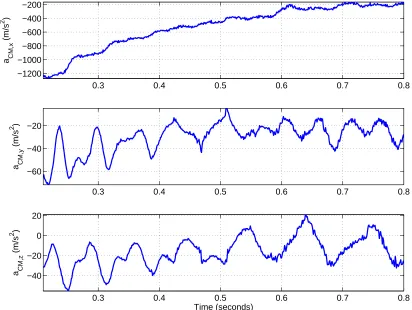
Figure 3.4: Filtered angular rate gyroscope output from CEV-TM-4
3.1 Transformations
Transforming the inertial velocities obtained by the radar to the body-xed reference frame yields the velocity components that may be used to determine angle of attack, sideslip angle, and total angle of attack [14].
Vx Vy Vz
→
u v w
α= arctanw
u
β = arcsin
v
√
u2+v2+w2
αT = arccos (cosαcosβ)
A series of transformations must rst be carried out. Many reference frames exist for describing projectile motion but they all follow the same basic denition, requiring an origin, a fundamental plane (which usually denes the z-axis) and a fundamental direction. Of the four used in the determination of the vehicle orientation three are inertial and the fourth is in the body reference frame. The range coordinate system is the system in which the radar data is presented; the origin is located at the muzzle, the fundamental plane is parallel to the local gravitational eld vector, and the fundamental direction is perpendicular to this plane in the same direction as the gun. The x-axis (downrange) is dened by the projection of the gun barrel onto the surface of the Earth. The y-axis (altitude) is in the fundamental plane and points up, measuring altitude. The z-axis (drift) is the cross-product of the x and y axes and completes the coordinate system. The origin of this system is the gun barrel exit. The next inertial reference frame is the North-East Down (NED) coordinate system, and is oriented such that the x-axis is pointed North and the y-axis is pointed East. The cross-product of these two axes yields the z-axis, which points into the Earth. The third coordinate system is the
magnetic eld (B) coordinate system and is dened as having the z-axis in the direction
fundamental direction is the North axis projected onto this fundamental plane. In this
coordinate system, the magnetic eld unit vector is dened as −→B =
0 0 1 T
. This intermediate coordinate system allows the magnetometers to be used directly in attitude determination. The nal coordinate system is the body-xed coordinate system in the body reference frame. This system is xed such that the origin is the projection of the center of mass onto the axial line of symmetry. The fundamental direction (x-axis) is along the vehicle axial line of symmetry and points toward the heat shield. The y and z-axes are in the fundamental plane which is orthogonal to the fundamental direction. The z-axis intersects the mass oset. Because this test test article did not have a mass oset, the z-axis was dened by the orientation of the CEV-TM package in the sabot. The y-axis is consistent with right-hand-rule coordinate systems.
A 2-1 rotation sequence (rst rotate about the range y-axis, then the intermediate x-axis) rotates the range coordinate system to the NED coordinate system.
DCMRange→N ED =
cosγ 0 −sinγ
sinγ 0 cosγ
0 −1 0
(3.1)
where γ is the azimuth of the gun. Rotation from the NED to the B-system involves a
3-2 rotation sequence.
DCMN ED→B =
cosδsini sinδsini −cosi
−sinδ cosδ 0
cosδcosi sinδcosi sini
(3.2)
Figure 3.6: Rotation between NED and magnetic eld coordinate systems
Rotating from the B-system to the body coordinate system involves a 3-2-1 rotation [15]. This direction cosine matrix (DCM) was used later on in the derivation of the kinematic relations.
DCMB→body =
cosψcosθ sinψcosθ −sinθ
cosψsinθsinφ−sinψcosφ sinψsinθsinφ+ cosψcosφ cosθsinφ
cosψsinθcosφ+ sinψsinφ sinψsinθcosφ−cosψsinφ cosθcosφ
(3.3)
where ψ, θ, and φ are the Euler angles corresponding to rotations about the z-axis,
Figure 3.7: Rotation between magnetic eld and body coordinate systems
Orientation can be determined through the relationship between the angular rates and the Euler angles and by the denition of the magnetic eld coordinate system. From examination of the DCM and the denition of the magnetic eld vector in the B-system, relations between normalized sensor measurements and Euler angles can be written.
θ = arcsin (−Bx)
φ = arctan
By
Bz
Note that ψ cannot be unambiguously determined from the magnetometers alone. A
the body-xed coordinate system allows the kinematic relations to be written as follows: ˙ φ ˙ θ ˙ ψ =
1 sinφtanθ cosφtanθ
0 cosφ −sinφ
0 sincosφθ coscosφθ p q r
where p, q, and r are the angular rate measurements of the body. From here, the
expression that relates the time derivative of ψ to the other two Euler angles and the
angular rates can be extracted [16].
˙
ψ = qsinφ+rcosφ cosθ
Integrating this expression yields the nal Euler angle.
ψ =ψ0 +
Z ˙
ψdt=ψ0+
Z
qsinφ+rcosφ
cosθ dt
This set of Euler angles now completes a chain of rotations from the range system to the body, permitting the velocities measured by the radar to be rotated to the body coordinate system. u v w
=DCMB→bodyDCMN ED→BDCMRange→N ED Vx Vy Vz (3.4)
These body-centered velocities can now be used to calculate angle of attack, sideslip angle, and total angle of attack.
of the high-g shock loads and the subsequent settling time of the angular rate gyros, this initial orientation is unknown. What is known is that the total torque derived from the moments of inertia and the angular rates and the total angle of attack should be in phase.
An iterative method was used to determine theψ0 needed to shift the values of total angle
of attack into phase with total torque. Comparing the normalized (to maximum value) angles of attack to the normalized torque leads to the minimum error solution.
0.3 0.4 0.5 0.6 0.7 0.8 0.2
0.4 0.6 0.8 1
Normalized Parameters
Normalized α
T
Normalized torque
0.3 0.4 0.5 0.6 0.7 0.8 −0.5
0 0.5
Time (seconds)
Difference
Figure 3.8: Comparison of normalized phase-correcting parameters
0.3 0.4 0.5 0.6 0.7 0.8 −20
−10 0 10 20
α
(degrees)
0.3 0.4 0.5 0.6 0.7 0.8 −20
0 20
β
(degrees)
0.3 0.4 0.5 0.6 0.7 0.8 10
20 30
α t
(degrees)
Time (seconds)
Figure 3.9: CEV ight angles generated by minimum error solution
3.2 Determination of Aerodynamic Coecients
The aerodynamic coecients are determined from the normal and axial forces and torques observed in the vehicle.
FN =m q
a2
CM,y +a2CM,z
The magnitude of the velocity is used to determine the dynamic pressure, and the ge-ometry of the vehicle is used to determine the reference area, which are both used to nondimensionalize the coecients.
V∞=
q
V2
x +Vy2+Vz2
q∞=
1 2ρ∞V
2
∞
S =πr2
Nondimensionalizing the forces and torques leads to the following coecients:
CN = qF∞NS , CA = qF∞AS
Cl= q∞LSd , Cm = q∞MSd , Cn= q∞NSd
Using the angle of attack as a rotation angle, the coecients of lift and drag are deter-mined [14].
CL=CNcosαT −CAsinαT
CD =CAcosαT +CNsinαT
The derivatives of the coecients of lift and the moment coecients are taken with
respect to the angle of attack, yielding stability terms. Note that for static stability,Cmα
3.3 Performance of Methodology
0.3 0.4 0.5 0.6 0.7 0.8 0.05
0.1 0.15 0.2
Time (seconds)
C N
10 20 30 0.05
0.1 0.15 0.2
αt (degrees)
C N
0.3 0.4 0.5 0.6 0.7 0.8 −0.5
−0.4 −0.3 −0.2 −0.1 0 0.1
Time (seconds)
C L
10 20 30 −0.5
−0.4 −0.3 −0.2 −0.1 0 0.1
αt (degrees)
C L
0.3 0.4 0.5 0.6 0.7 0.8 −0.04
−0.02 0 0.02 0.04
Time (seconds)
C m
−20 −10 0 10 20 −0.04
−0.02 0 0.02 0.04
α (degrees)
C m
0.3 0.4 0.5 0.6 0.7 0.8 −0.06
−0.04 −0.02 0 0.02 0.04 0.06
Time (seconds)
C n
−20 0 20 −0.06
−0.04 −0.02 0 0.02 0.04 0.06
β (degrees)
C n
Figure 3.11: CEV pitching and yawing moment coecients
Note that there are fairly distinct regions illustrated, particularly for the normal force coecient, that indicate a shift from supersonic to transonic and subsonic dynamics,
oc-curring around 0.5 seconds. The negativeCmα and positiveCnβ imply static longitudinal
and lateral stability. Coecients were compared to available values generated by the EXTRACTR 6-DOF maximum likelihood estimator [17].
Table 3.1: Comparison of coecients between analytical method and EXTRACTR Analytic EXTRACTR Percent Dierence
CNα 0.23 0.20 15%
Cmα -0.10 -0.10 0%
CA0 1.21 1.47 18%
Chapter 4
Aeroballistic Testing with Pressure
Transducers
After the initial series of tests, it was decided that the project may benet in transi-tioning from the use of a 120mm smooth-bore cannon to a 7-inch (approximately 180mm) High Altitude Research Program (HARP) gun. This change in test apparatus enables the use of a larger test article, with more internal volume available for instruments and a greater ballistic coecient, thus extending the duration of usable free-ight data.
made on each primary axis throughout the ight. For the purposes of these aeroballistic tests, one of the magnetometers was subjected to a single auto set/reset approximately 1 second after initial power up while the second unit was subjected to a series of pre-programmed set/resets regularly throughout the ight to investigate changes in biases and scale factors that may have occurred during the ight. Four accelerometers were placed at a radial oset from the symmetric axis and the outputs were summed in an attempt to approximate the spin rate of the body. One channel was used to monitor the on-board battery.
This increase in the number of recordable channels and the overall increase in test article size supported the installation of MEMs-based pressure transducers within the telemetry module, the now renamed CEV pressure telemetry module or CEV-PTM [18].
Figure 4.1: Diagram of CEV-PTM
transducers were measured and recorded on two channels to check that the pressure transducers were operating within temperature uctuation tolerance levels.
4.1 Pressure Transducers
Aeroballistic tests conducted with fore-body pressure monitoring for the purpose of determining test article ight parameters have never been documented before. The high shock loads encountered during ring and the eects such loads may have on a pres-sure transducer requires thorough research into available prespres-sure transducers and their limitations and physical experimentation on pressure transducers as a prelude to ight testing.
Most pressure transducers operate by measuring the deection of a diaphragm. Cali-bration curves are used to determine how much pressure is required to induce an observed diaphragm deection. This can be accomplished electronically in the form of a semicon-ductor by measuring the change of a electronic property (resistance or capacitance, for example) due to the deection of a piezoelectric material [19]. This allows for the minia-turization of pressure transducers to a scale more suitable to the volumetric constraints of aeroballistic test articles.
eects on the diaphragms must be considered. The transducer package size must be small enough to t within the volumetric constraints of the test article. The size of the pressure transducer aects its oset from the CM forebody, determining the depth of the pressure tap. This is important as aeroballistic tests collect data in real-time; the potential exists for lag times to appear in collected pressure measurements.
The Kulite XCEL-100 series of sealed gage pressure transducers, manufactured by Kulite Semiconductor Products, Inc., best t the operating criteria of the Orion CM aeroballistic tests [20].
NOTE: FOR INTERNAL COMPENSATION CONSULT FACTORY CONSULT FACTORY FOR SPECS. ON SEALED GAGE
123
KULITE SEMICONDUCTOR PRODUCTS, INC. • One Willow Tree Road • Leonia, New Jersey 07605 • Tel: 201 461-0900 • Fax: 201 461-0990 • http://www.kulite.com
Continuous development and refinement of our products may result in specification changes without notice - all dimensions nominal. (O)
Note: Custom pressure ranges, accuracies and mechanical configurations available. Dimensions are in inches. Dimensions in parenthesis are in millimeters.
HIGH TEMPERATURE
MINIATURE IS
®PRESSURE TRANSDUCER
XCEL-100 SERIES
•
.101" Diameter
•
Patented Leadless Technology
•
Ideal For Turbine Engine Probes
•
Designed For Both Static and Dynamic Measurement
•
– 65°F To 525°F Temperature Capability
The XCEL-100 design features Kulite's patented leadless technology. This allows for a very rugged package suited for probes, pressure rakes and other similar test set ups. This transducer is well suited for both dynamic and static pressure measurements in benign or harsh environments. Its wide operating temperature range (-65°F to +525°F) makes it ideal for numerous applications in Aerospace and other areas of Industry.
.375 (9.5)
4 LEADSTEFLON INSULATED #36 AWG 24" (610) LONG BEFORE COMP. MODULE
4 LEADSTEFLON INSULATED #36 AWG 12" (305) LONG AFTER COMP. MODULE .101
(2.6) PRESSURE REFERENCE TUBE.016 O.D. X 1” LONG
(.41 X 25.4) FOR PSIG & PSID UNITS
B SCREEN STANDARD M SCREEN OPTIONAL
G N I R I W R O L O
C DESIGNATION
D E
R +INPUT
K C A L
B – INPUT
N E E R
G +OUTPUT
E T I H
W – OUTPUT
INPUT
Pressure Range 0.355 1.015 1.725 3.550 1007 20014 30021 50035 1000 PSI70 BAR
Operational Mode Absolute, Gage, Sealed Gage, Differential Absolute, Sealed Gage
Over Pressure 2 Times Rated Pressure
Burst Pressure 3 Times Rated Pressure
Pressure Media All Nonconductive, Noncorrosive Liquids or Gases (Most Conductive Liquids and Gases - Please Consult Factory)
Rated Electrical Excitation 10 VDC/AC
Maximum Electrical Excitation 15 VDC/AC
Input Impedance 1000 Ohms (Min.)
OUTPUT
Output Impedance 1000 Ohms (Nom.)
Full Scale Output (FSO) 100 mV (Nom.)
Residual Unbalance ± 5 mV (Typ.)
Combined Non-Linearity, Hysteresis
and Repeatability ± 0.1% FSO BFSL (Typ.), ± 0.5% FSO (Max.)
Resolution Infinitesimal
Natural Frequency (KHz) (Typ.) 150 175 240 300 380 550 575 700 1000
Acceleration Sensitivity % FS/g Perpendicular Transverse 1.5x10 -3 2.2x10⁻⁴ 1.0x10⁻³ 1.4x10⁻⁴ 5.0x10⁻⁴ 6.0x10⁻⁵ 3.0x10⁻⁴ 4.0x10⁻⁵ 1.5x10⁻⁴ 2.0x10⁻⁵ 1.1x10⁻⁴ 1.5x10⁻⁵ 9.0x10⁻⁵ 1.0x10⁻⁵ 6.0x10⁻⁵ 6.0x10⁻⁶ 4.0x10⁻⁵ 4.0x10⁻⁶
Insulation Resistance 100 Megohm Min. @ 50 VDC
ENVIRONMENTAL
Operating Temperature Range -65°F to +525°F (-55°C to +273°C)
Compensated Temperature Range +80°F to +450°F (+25°C to +235°C)
Thermal Zero Shift ± 1% FS/100°F (Typ.)
Thermal Sensitivity Shift ± 1% /100°F (Typ.)
Steady Acceleration and Linear
Vibration 1000g Sine
PHYSICAL
Electrical Connection 4 Leads 36 AWG 36" Long
Weight .4 Gram (Nom.) Excluding Module and Leads
Pressure Sensing Principle Fully Active Four Arm Wheatstone Bridge Dielectrically Isolated Silicon on Silicon Patented Leadless Technology
Figure 4.2: Kulite XCEL-100 pressure transducer
4.2 Pressure Transducer Calibration
The test article has been designed to support up to ten pressure transducers, one being a blind transducer (receives no airow) that was used to quantify pressure errors due to acceleration. In general, the manufacturer-supplied sensitivity calibration curves were used for each transducer. Pre-ight calibration procedures have been documented to ensure that the transducers are functioning before and after they have been potted (permanently xed within the test article) and that the ports are clear. The test article was placed within a pressure vessel and a static calibration over stepped pressure values performed to a maximum allowable pressure (supply air limitation) of 827,370 Pascals (120psi). Sensor data was telemetered out of the pressure vessel to a receiving station and recorded. This calibration allowed the evaluation of the seals between transducer ports; the dummy transducer should measure no pressure change if the seals are sucient. The custom calibration curves and conguration of each transducer warrants this system-level static calibration, as each transducer relies on a compensation circuit made up of three resistors, with each transducer having unique resistor values.
-101 0 10 20 30 40 50 60 70 80 2
3 4 5 6 7 8 9x 10
5 Pressure Tap #3
Pressure (pascals)
time (seconds)
Figure 4.3: CEV-PTM-01 static pressure calibration response
Chapter 5
Constructing an Aerodynamic
Database
To determine ight parameters of the Orion CM test article from aeroballistic pressure measurements, an aerodynamic database must be constructed. An aerodynamic database contains information that relates pressure measurements at various locations on a body to parameters of interest, like Mach number and vehicle orientation. The data used to construct an aerodynamic database typically comes from static testing, such as those conducted by wind tunnels. This data may be used to validate CFD codes. Such wind tunnel tests were conducted on the Orion CM geometry.
5.1 Wind Tunnel Testing
Figure 5.1: NASA Ames Unitary Plan Wind Tunnel
Both facilities are closed-circuit, variable-pressure, continuous operation wind tunnels with multiple legs. For the AUPWT, subsonic Mach number control in the 11x11 leg is achieved with a combination of compressor drive speed control and variable-camber guide vanes at the compressor inlet. Supersonic Mach number control additionally involves setting the exible wall nozzle to achieve the proper area ratio. This leg of the tunnel can be operated between Mach number of 0.2 to 1.45. The 9x7 leg can vary Mach number between 1.5 and 2.5 by means of a sliding block inlet which forms the oor of an S-shaped duct. Sliding the block forward or back controls area ratio, changing the ow conditions in the test section [21].
with respect to overall model dimensions. Static pressures at each tap are measured using multiple (facility-dependent) calibrated pressure tap scanning devices, connected to each tap using pressure tubing, which is housed within the sting apparatus to minimize aerodynamic interference. Boundary layer trip dots were applied to all models. This consisted of an approximated circle (trip dot tape can only be applied in a straight line) of trip dots which enclosed the stagnation point over its expected range of variation with angle of attack.
Figure 5.2: Wind tunnel CM model with sting assembly and trip dots
Each model was tested over a Mach number range of 0.3 to 2.5 and a Reynolds number
range of 1.5×10⁶ to 5.3×10⁶. Reynolds number values play a signicant role in the
transition from laminar to turbulent ow and in the subsequent changes in force and moment values. The sting was mounted to a knuckle-sleeve assembly which rotated the model through a range of angles of attack. Angle of attack is considered equivalent to total angle of attack, unless accompanied by another angle. Limitations on the sting range-of-motion prevented sideslip angle variation [21]. As this is an axisymmetric body, symmetry arguments may be used in determining resultant forces, moments, and pressure distributions given a sideslip angle. Small deections due to loads acting on the sting arm induced small sideslip angles on the order of one-tenth of a degree and are considered negligible.
5.2 Computational Fluid Dynamics Simulations
Computational uid dynamics (CFD) relies on discretized mathematical models and iterative processes to approximate the expected oweld surrounding a body, given a set of initial parameters. Such models can be used to interpolate over the parameters used and the results obtained from physical experimentation, like wind tunnel tests. These models must rst be validated by these tests before results can be used in further analysis. Various CFD codes exist and appropriate uses are bounded by the assumptions in-herent in the algorithms and structures of the codes and the sort of body being analyzed. All codes are various attempts to iteratively solve the Navier-Stokes equations.
scalable computing resources. It employs a discretization model that partitions the ow-eld into near-body and o-body regions. The near-body region includes the surface geometry of all bodies being considered and the volume of space extending a short dis-tance above the respective surfaces. The o-body region encompasses the near-body domain and extends to the far-eld boundaries of the problem, with grid resolution de-termined based on proximity to near-body components [22]. The OVERFLOW-D solver was used to approximate the oweld surrounding the Orion CM geometry over an ex-tended range of Mach and Reynolds numbers and angles of attack, allowing comparison to wind tunnel data and extrapolation beyond the capabilities of available wind tunnel facilities.
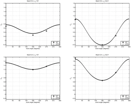
Figure 5.3: CFD and wind tunnel test range and grid/tap locations on Orion CM fore-body
0 45 90 135 180 225 270 315 360 -0.2 0 0.2 0.4 0.6 0.8 1 1.2 1.4 1.6 1.8
clock angle (degrees) CP
Mach=0.5,DT=10q
WT CFD
0 45 90 135 180 225 270 315 360
-0.2 0 0.2 0.4 0.6 0.8 1 1.2 1.4 1.6 1.8
clock angle (degrees) CP
Mach=0.5,DT=32.5q
WT CFD
0 45 90 135 180 225 270 315 360
-0.2 0 0.2 0.4 0.6 0.8 1 1.2 1.4 1.6 1.8
clock angle (degrees) CP
Mach=2.5,D
T=10q
WT CFD
0 45 90 135 180 225 270 315 360
-0.2 0 0.2 0.4 0.6 0.8 1 1.2 1.4 1.6 1.8
clock angle (degrees) CP
Mach=2.5,D
T=32.5q
WT CFD
Figure 5.4: CFD and wind tunnel pressure coecient variation at cone angle of 19.45-degrees
more gridpoints and has a larger Mach range. Both sets of data must be reconciled in developing an aerodynamic database.
5.3 Development of an Analytic Pressure Model
Development of an analytic model that yields a pressure value given Mach number, ight angles, and tap location is critical to developing a method to obtain these ight pa-rameters from pressure tap measurements. Oftentimes, a multidimensional interpolation is conducted to determine the ight parameters given a series of pressure measurements at a given time. This method has some limitations to take into account:
Solutions for parameters may be incorrect given a sparse database
Multiple solutions may exist for a given set of pressures
Does not force physical constraints (symmetry is not required)
Cannot resolve multiple data sources with discrepancies
Multidimensional interpolation is computationally expensive
Developing an analytic model as a function of tap location and ight parameters using CFD data, then anchoring this model to wind tunnel data, which is sparse in clock
angle, φ, resolves the two sets of data and yields a model that allows the determination
of ight parameters given a series of pressure transducer data. The available wind tunnel data was assumed to more accurately depict the surface pressure values across the CM forebody, particularly around the stagnation point.
between pressure coecient and clock angle. A series in cosine was used to model the distribution with the appropriate number of terms in the series carefully selected. Too few terms may not capture all of the variation in the data with respect to clock angle, but too many terms may introduce high-frequency artifacts that do not represent the data. Based on the number of maxima and minima in the pressure coecient data with respect to clock angle, a three-term series in cosine was found to be sucient.
CP =a1+a2cosφ+a3cos 2φ (5.1)
This series minimizes the error and is easily solved for the coecients.
0 50 100 150 200 250 300 350
1 1.1 1.2 1.3 1.4 1.5 1.6 1.7
clock angle (degrees)
CP
CFD Data 3 coefficients 2 coefficients 4 coefficients
0 50 100 150 200 250 300 350
-0.02 -0.015 -0.01 -0.005 0 0.005 0.01 0.015 0.02
clock angle (degrees)
Δ
CP
3 coefficients 2 coefficients 4 coefficients
Increasing the number of terms to four does not noticeably improve the residuals. For the range of available Mach numbers and angles of attack, the error is small, with a maximum error of approximately 3%.
Figure 5.6: Percent dierence of CFD 3-term analytical model
Figure 5.7: Quadratic relationship between angle of attack and 3-term model coecients
The full analytic model for pressure coecient as a function of tap location, Mach number, and total angle of attack can now be written, where the coecients are functions of Mach number and cone angle.
CP =c1+αT (c2+αTc3) +αT (c4+αTc5) cosφ+αT (c6+αTc7) cos 2φ (5.2)
error varies between 1% and 2% at lower Mach numbers.
Figure 5.8: Percent dierence of CFD 7-term analytical model
The wind tunnel tests and CFD simulations only varied angle of attack, which the analytical model treats as total angle of attack. Sideslip angles are not likely to be zero, and must be included in the model. Because the analytic model is continuous in clock angle, the angle of attack and sideslip angle were represented as a total angle of attack
and an additional rotational term, ψ, which is added to the clock angle of the pressure
tap.
αT = arccos (cosαcosβ) α = arcsin (cosψsinαT)
ψ = arctan cossinαsinα β β = arctansinαTsinψ
cosαT
CP =c1+αT (c2+αTc3)+αT (c4+αTc5) cos (φ+ψ)+αT (c6+αTc7) cos 2 (φ+ψ) (5.3)
It was necessary to develop the analytic model using the CFD data because the wind tunnel data is sparse in clock angle; there are only three available data points, four using symmetry arguments. The coecients obtained using the CFD data were corrected to anchor the model to the wind tunnel data points while maintaining the same functional form. The correction terms are simply partial derivatives of the analytic model with respect to the coecients.
c1 · · · c7
=
c1 · · · c7
CF D +
δCPmodel c1 · · ·
δCPmodel c7
... ... ...
CPW T −CPCF D
...
0 45 90 135 180 225 270 315 360 -0.2 0 0.2 0.4 0.6 0.8 1 1.2 1.4 1.6 1.8
clock angle (degrees) CP
Mach=0.5,DT=10q
WT Analytic Model CFD (7 coefficient model)
0 45 90 135 180 225 270 315 360
-0.2 0 0.2 0.4 0.6 0.8 1 1.2 1.4 1.6 1.8
clock angle (degrees) CP
Mach=0.5,DT=32.5q
WT Analytic Model CFD
0 45 90 135 180 225 270 315 360
-0.2 0 0.2 0.4 0.6 0.8 1 1.2 1.4 1.6 1.8
clock angle (degrees) CP
Mach=2.5,D
T=10q
WT Analytic Model CFD
0 45 90 135 180 225 270 315 360
-0.2 0 0.2 0.4 0.6 0.8 1 1.2 1.4 1.6 1.8
clock angle (degrees) CP
Mach=2.5,D
T=32.5q
WT Analytic Model CFD
Figure 5.9: Anchored analytical model compared to unanchored model and wind tunnel datapoints at cone angle of 19.45-degrees
Note that the available wind tunnel data does not exceed Mach 2.5. The coecients obtained using the CFD data beyond this Mach number remain unchanged, with the average of the coecients obtained using CFD data and the wind-tunnel-anchored coef-cients taken at Mach 2.5; eectively the CFD-based coecoef-cients corrected by half of the obtained correction term at Mach 2.5.
coecient. The analytic model was rewritten to reect this.
CP =
P −P∞
q∞
= P1−P∞
2ρV 2
∞
→P = 1
2CPρ∞V
2
∞+P∞ (5.5)
V∞ can be rewritten in terms of known parameters.
V∞ =M a
a=√γRT∞
→V∞=M
p
γRT∞
P = 12CPρ∞M2γRT∞+P∞
P∞=ρ∞RT∞
→P = 1
2CPM
2γP
∞+P∞
The analytical model is now a function of only two atmospheric parameters, atmospheric pressure and the atmospheric ratio of specic heats.
P = P∞
2 2 +γCPM
2
(5.6)
The analytic model as derived is based on wind tunnel data, while deriving its functional form from CFD data. Symmetry constraints were maintained and the coecients may be easily interpolated over Mach number, as cone angle is a known and xed parameter for the pressure transducers.
5.4 Pressure Tap Placement
distance between symmetrically-opposed taps about the axis of symmetry. The dier-ence between these pressures should be zero at 0-degrees angle of attack and a positive or negative value based on a non-zero angle of attack, where the angle is in the same plane as the two tap and the symmetric axis. By this argument, taps should be placed as far apart as possible from each other, each one on the edge of the heatshield-cone shoulder. Uncertainties associated with Mach number and ight angle determination based on these pressures would likely be high as the oweld in the shoulder region of the CM is quite turbulent.
Stagnation point location is a key factor in determining pressure tap locations. The
cone angle, λ, of the maximum pressure coecient is a well-dened function in angle of
0 5 10 15 20 25 30 35 40 0
5 10 15 20
total angle of attack (degrees)
cone angle (degrees)
Figure 5.10: Stagnation point cone angle over a range of angles of attack at varying Mach numbers
This location is weakly sensitive to Mach number variation. The supersonic and subsonic design trim angles of attack of the CEV-PTM are 21.46-degrees and 12.21-degrees [23]. These values correspond to Mach numbers of 2.5 and 0.7. For the pressure transducers to measure the stagnation pressure during the aeroballistic test, pressure taps should be placed at a cone angle of 12.59-degrees.
in which wind tunnel and CFD pressure coecient data are within 10% of each other suciently addresses this issue.
-25-22.5-20-17.5-15-12.5-10 -7.5 -5 -2.5 0 2.5 5 7.5 10 12.5 15 17.5 20 22.5 25 -2 -1.5 -1 -0.5 0 0.5 1 1.5 2
CEV Vertical Plane: Mach=0.5, D
T=10q
CP
CFD WT
-25-22.5-20-17.5-15-12.5-10 -7.5 -5 -2.5 0 2.5 5 7.5 10 12.5 15 17.5 20 22.5 25 -10
0 10
cone angle, with (-) sign corresponding to clock angle of 180q (degrees)
'
CP
%FS
CFD
-25-22.5-20-17.5-15-12.5-10 -7.5 -5 -2.5 0 2.5 5 7.5 10 12.5 15 17.5 20 22.5 25 -2 -1.5 -1 -0.5 0 0.5 1 1.5 2
CEV Horizontal Plane: Mach=0.5, D
T=10q
CP
CFD WT
-25-22.5-20-17.5-15-12.5-10 -7.5 -5 -2.5 0 2.5 5 7.5 10 12.5 15 17.5 20 22.5 25 -10
0 10
cone angle, with (-) sign corresponding to clock angle of 90q (degrees)
'
CP
%FS
CFD
-25-22.5-20-17.5-15-12.5-10 -7.5 -5 -2.5 0 2.5 5 7.5 10 12.5 15 17.5 20 22.5 25 -2 -1.5 -1 -0.5 0 0.5 1 1.5 2
CEV Vertical Plane: Mach=2.5, DT=10q
CP
CFD WT
-25-22.5-20-17.5-15-12.5-10 -7.5 -5 -2.5 0 2.5 5 7.5 10 12.5 15 17.5 20 22.5 25 -10
0 10
cone angle, with (-) sign corresponding to clock angle of 180q (degrees)
'
CP
%FS
CFD
-25-22.5-20-17.5-15-12.5-10 -7.5 -5 -2.5 0 2.5 5 7.5 10 12.5 15 17.5 20 22.5 25 -2 -1.5 -1 -0.5 0 0.5 1 1.5 2
CEV Horizontal Plane: Mach=2.5, DT=10q
CP
CFD WT
-25-22.5-20-17.5-15-12.5-10 -7.5 -5 -2.5 0 2.5 5 7.5 10 12.5 15 17.5 20 22.5 25 -10
0 10
cone angle, with (-) sign corresponding to clock angle of 90q (degrees)
'
CP
%FS
CFD
Figure 5.11: Comparison of CFD and wind tunnel Orion CM data on vertical and hori-zontal planes
This agreement is maintained up to a maximum cone angle of 19.45-degrees. This is the largest cone angle at which pressure taps may be placed while maintaining agreement between CFD and wind tunnel data sources, which implies that turbulent ow eld eects at the shoulder are minimized.
Chapter 6
Parameter Estimation
The analytic pressure model may be used to compute the ight parameters, Mach number, angle of attack, and sideslip angle. A variety of approaches were investigated that all focused on iterative solutions to a standard matrix problem for a series of un-knowns.
6.1 Least Squares Approach
Given pressure data, the least squares method can be used to determine the value of the parameters at a point in time
M α β n+1 = M α β n
+ BTB−1BT {y}
B = δP δM T ap1
δP δα
T ap1
δP δβ
T ap1
δP δM
T ap2
δP δα
T ap2
δP δβ
T ap2
... ... ...
δP δM
T ap i
δP δα
T ap i
δP δβ
T ap i
{y}=
PmeasuredT ap1 −PcomputedT ap1 PmeasuredT ap2 −PcomputedT ap2
...
PmeasuredT ap i−PcomputedT ap i
As the model is linear in two of the three parameters, the necessary elements of the matrix of partial derivatives of pressure with respect to angle of attack and sideslip angle may be calculated analytically. A central nite dierence was used to determine the partial derivative of pressure with respect to Mach number.
This method works by nding the optimal combination of parameters in the 3-dimensional space that minimizes the residual pressure. The feasibility of the solution is improved by using the previous closest local minimum as the initial value for the next time step. This does not take into account the eects of real-world phenomena that are readily observable in measured data: scale factor, bias, and noise eects.
Pmeasured=sPactual+b+noise (6.1)
Thousands of datapoints may be generated from an aeroballistic ight test in the region of interest, in this case for the range of Mach numbers between barrel exit and 0.5. Solving for the local ight parameters at each time is a computationally simple operation, while solving for the global parameters of scale factor and bias requires much more memory and unnecessary matrix calculations. Available memory rapidly becomes a constraining factor when manipulating matrices that possess hundreds of thousands of elements. A back-substitution method was employed to work around this issue.
Consider two sets of nine pressure measurements (taken from the CEV-PTM pressure
tap cruciform), corresponding to timestampst1 and t2. This corresponds to 9 individual
scale factors and biases and 2 pairs of 3 ight parameters.
X0 =
sT ap1 sT ap2 · · · sT ap9 bT ap1 bT ap2 · · · bT ap9
T
X1 =
Mt1 αt1 βt1
X2 =
Mt2 αt2 βt2
The parameters of interest, 24 in all, may be written as a single vector.
X = X0 X1 X2
be generated.
Ai = δP δsT ap1
T ap1
· · · δP δsT ap9
T ap1
δP δbT ap1
T ap1
· · · δP δbT ap9
T ap1
δP δsT ap1
T ap2 · · ·
δP δsT ap9
T ap2
δP δbT ap1
T ap2 · · ·
δP δbT ap9
T ap2
... ... ... ... ... ...
δP δsT ap1
T ap9 · · ·
δP δsT ap9
T ap9
δP δbT ap1
T ap9 · · ·
δP δbT ap9
T ap9
Bi = δP δM T ap1
δP δα
T ap1
δP
δβ
T ap1
δP δM
T ap2
δP δα
T ap2
δP
δβ
T ap2
... ... ...
δP δM
T ap i
δP δα
T ap i
δP δβ
T ap i i
yi =
PmeasuredT ap1 −PcomputedT ap1 PmeasuredT ap2 −PcomputedT ap2
...
PmeasuredT ap i −PcomputedT ap i
i
Ai and Bi are 9 by 18 and 9 by 3 matrices of partial derivatives corresponding to the
bias and scale factor parameters and the ight parameters, respectively. yi is the 18 by
1 vector of pressure residuals. These matrices and vectors may be used to construct a system-level (ight parameters at each time step and scale factors and biases) sensitivity matrix and residual vector.
J =
A1 B1 0
A2 0 B2
y= y1 y2
This leads to an expression for the least squares solution.
JTJδX =JTy (6.2)
δX is the vector of correction terms on each of the parameters. Note that J is
rank-decient unless three sets of data are used. As an accumulative method is being devel-oped, two sets of data will be sucient for this derivation.
These matrices may now be evaluated and expanded.
JTJ = AT
1A1+AT2A2 AT1B1 AT2B2
B1TA1 BT1B1 0
B2TA2 0 B2TB2
JTy=
AT1y1+AT2y2
BT
1y1
BT
2y2
AT1A1 +AT2A2
δX0+AT1B1δX1+AT2B2δX2 =AT1y1+AT2y2 (6.3)
B1TA1δX0+B1TB1δX1 =B1Ty1 (6.4)
Equations 6.4 and 6.5 may be rearranged, resulting in a two equations that relate the residuals and sensitivity matrices to correction terms on the scale factors and biases.
δX1 = B1TB1
−1
BT1y1− BT1B1
−1
B1TA1δX0 (6.6)
δX2 = B2TB2
−1
BT2y2− BT2B2
−1
B2TA2δX0 (6.7)
Note that the rst term in each equation is the least squares solution when bias and scale
factor are omitted, δXei. Substituting δX1 and δX2 into 6.3 and rearranging,
AT1A1+AT2A2
δX0+AT1B1
δXe1− B1TB1 −1
B1TA1δX0
+AT2B2
δXe2− B2TB2 −1
B2TA2δX0
=AT1y1+AT2y2
AT1A1−AT1B1 B1TB1
−1
B1TA1+AT2A2−AT2B2 B2TB2
−1
BT2A2
δX0
=AT1y1 −AT1B1δXe1+AT2y2−AT2B2δXe2 (6.8)
tN
X
t1
ATtAt−ATtBt BtTBt −1
BtTAt
δX0 =
tN
X
t1
ATtyt−ATtBtδXet
δX0 =
tN
X
t1
ATtAt−ATtBt BtTBt −1
BtTAt
!−1 t
N
X
t1
ATtyt−ATtBtδXet
(6.9)
6.2 Minimum Variance Approach with A Priori
Oftentimes an a priori estimate of a set of parameters to be estimated is available. Such information may include specied parameter values and associated uncertainties. Uncertainties in measurements are typically known. This information may be used to implement a minimum variance approach that incorporates this a priori knowledge [25].
JTΓ−1J+ Γ−µ1
δX =JTΓ−1y+ Γ−µ1(µ−X) (6.10)
In this equation,µ is the a priori estimate of the parameters. Γµ is the a priori estimate
of the covariance matrix and is assumed to be diagonal.
Γ−µ1 =
σM2 0 0 0 σ2
α 0
0 0 σ2
β −1
Γ−1is the the inverse of the variance of the pressure measurements. Equation 6.10 may
be simplied by distributing this variance term across the matrices.
Γ−1 = Γ−1/2
Γ
−1/2
ˆ
J = Γ−1/2J, yˆ= Γ−
1/2
y
ˆ
JTJˆ+ Γ−µ1
δX = ˆJTyˆ+ Γ−µ1(µ−X) (6.11)
As demonstrated earlier, a back-substitution method may address memory concerns associated with the computationally expensive matrix manipulations required to simul-taneously solve for the scale factors, biases, and ight parameters. Applying this method to the minimum variance with a priori approach is fairly straight-forward. Consider data
obtained from a 9-tap cruciform. As before, J is the sensitivity matrix associated with
both global and local parameters and y is the vector of residuals. Both are constructed from pressure measurements taken at two times, and both are normalized by the known
pressure variance. The a priori covariance matrix,Γ−µ1 and the vector of estimates, µ, are
augmented with the a priori estimates of the scale factors and biases.
µ= µ0 µ1 µ2
Γ−µ1 =
σµ2X
0 0 0
0 σ2
µX1 0
0 0 σ2
µX2
−1
ˆ
A1TAˆ1+ ˆAT2Aˆ2 +σµ−X20
δX0+ ˆAT1Bˆ1δX1+ ˆAT2Bˆ2δX2 = ˆA1Ty1+ ˆAT2y2 +σµ−X20 (µ0−X0)
(6.12)
ˆ
BT1Aˆ1δX0+
ˆ
B1TBˆ1+σµ−X21
δX1 = ˆB1Tyˆ1+σ−µX21 (µ1−X1) (6.13)
ˆ
BT2Aˆ2δX0+
ˆ
B2TBˆ2+σµ−X22
δX2 = ˆB2Tyˆ2+σ−µX22 (µ2−X2) (6.14)
Equations 6.13 and 6.14 may be rearranged, resulting in a two equations that relate the residuals and sensitivity matrices to correction terms on the scale factors and biases.
δX1 =
ˆ
B1TBˆ1+σ−µX21
−1 ˆ
B1Tyˆ1+σµ−X21 (µ1 −X1)
−Bˆ1TBˆ1+σ−µX21
−1 ˆ
B1TAˆ1δX0
(6.15)
δX2 =
ˆ
B2TBˆ2+σ−µX22
−1 ˆ
B2Tyˆ2+σµ−X22 (µ2 −X2)
−Bˆ2TBˆ2+σ−µX22
−1 ˆ
B2TAˆ2δX0
(6.16) Note that the rst term in each equation is the minimum variance solution when bias
and scale factor are omitted, δXei. Substituting δX1 and δX2 into 6.12 and rearranging,
ˆ
A1TAˆ1+ ˆAT2Aˆ2+σ−µX20
δX0+ ˆAT1Bˆ1
δXe1−
ˆ
B1TBˆ1+σµ−X21
−1 ˆ
B1TAˆ1δX0
+ ˆAT2Bˆ2
δXe2−
ˆ
B2TBˆ2+σ−µX22
−1 ˆ
B2TAˆ2δX0