ABSTRACT
LUO, SHA. Ordering Strategy, Supplier Incentive and Supply Chain Performance. (Under the direction of Dr. Russell E. King and Dr. Shu-Cherng Fang.)
A supply chain usually consists of different players/companies with conflicting objectives. In this dissertation, we concentrate on a two-echelon supply chain consisting of one retailer and multiple suppliers. We study particularly the interactive effects of the retailer’s sourcing strategy and suppliers’ wholesale pricing decisions. This dissertation consists of three essays, each looking into the supply chain with a different feature.
The first essay considers the retailer’s trade-off between selecting an unreliable, economic supplier and a reliable, expensive supplier with fixed ordering costs. We successfully provide mathematical proofs for an (s, S)-like optimal ordering policy in the finite-horizon setting. We also analyze the limiting behavior of the (s, S)-like policy to show that the converged policy characterizes the optimal ordering policy for the infinite-horizon setting. Extensive experimental results indicate that the (s, S)-like ordering policy is optimal under a wide range of system parameters beyond the conditions required in the optimality proof.
The second essay studies a short-life-cycle product supply chain with a normal supplier and a quick response supplier. As it approaches the selling season, more accurate demand updates become available. The retailer has the option of single sourcing or dual sourcing while the suppliers determine the unit wholesale price under a specific sourcing strategy revealed by the retailer. The retailer’s ordering and the suppliers’ pricing decisions are characterized using game theoretical approach. With an exponentially distributed demand, we find that the retailer prefers single sourcing to dual sourcing. We then consider introducing more QR suppliers and find that contribution benefits the supply chain.
© Copyright 2017 by Sha Luo
Ordering Strategy, Supplier Incentive and Supply Chain Performance
by Sha Luo
A dissertation submitted to the Graduate Faculty of North Carolina State University
in partial fulfillment of the requirements for the Degree of
Doctor of Philosophy
Industrial Engineering
Raleigh, North Carolina
2017
APPROVED BY:
Dr. Donald P. Warsing, Jr. Minor of Advisory Committee
Dr. Yunan Liu
DEDICATION
To my family: Youyu Zhang
BIOGRAPHY
ACKNOWLEDGEMENTS
I have been very fortunate to receive a lot of guidance, inspiration and encouragement during my Ph.D. study.
First of all, my deepest gratitude goes to my advisors, Dr. Russell King and Dr. Shu-Cherng Fang. I am very fortunate to have two advisors and get exposed to their different charismata. I am deeply indebted to Dr. King for offering me the opportunity to teach an undergraduate course and his mentorship during the teaching process. I benefited a lot from watching him teach and discussing my research topics with him. Despite his busy schedule, he always gives me the advice and guidance I need. He always has a lot of confidence in me and encourages me to excel myself. Dr. Fang not only serves as an academic supervisor but also a life mentor. Academically, he sets an example for me to be a rigorous scholar. Mentally, he shares his experience with me, enlightens me in daily life, and teaches me to be a caring and wise person by being one. Both Dr. King and Dr. Fang have a profound influence on me. It is truly my privilege to be one of their students.
I am deeply grateful for Dr. Donald P. Warsing and Dr. Yunan Liu for being members of my advisory committee and Dr. Thayer Morrill for serving as my graduate school representative. Especially, I want to thank Dr. Warsing, with whom I had the opportunity to collaborate on one paper. Working with him is indeed an enjoyable learning process.
I would also like to thank Dr. Zhe Liang, for bringing me into the wonderful world of Operations Research and Industrial Engineering, the selection committee for offering me the opportunity to study at NC State, Mr. Edward Fitts and the center for Additive Manufacturing and Logistics for financial support. My sincere thanks and appreciation also go to all the professors, especially those I have taken courses from, in ISE department. I enjoyed all the courses and have benefited a lot from their instructive teaching.
Wang, Chien-Chia Huang, Tiantian Nie, Mohamed Desoky, Jiahua Zhang, Qi An, Shan Jiang, Yu-Liang Lin, Chi-Yi Chen and many others. We had lunch together every Friday and have shared a lot of happy moments.
The two people I feel I am forever indebted to are my parents. I am very grateful to be raised in a democratic family. Different from many other Chinese parents, my parents never impose their willingness on me and they respect my opinions. They always encourage me to go to a bigger stage to excel myself, even if it means building a long distance between them and me. I could not have been where I am without their constant love and support.
TABLE OF CONTENTS
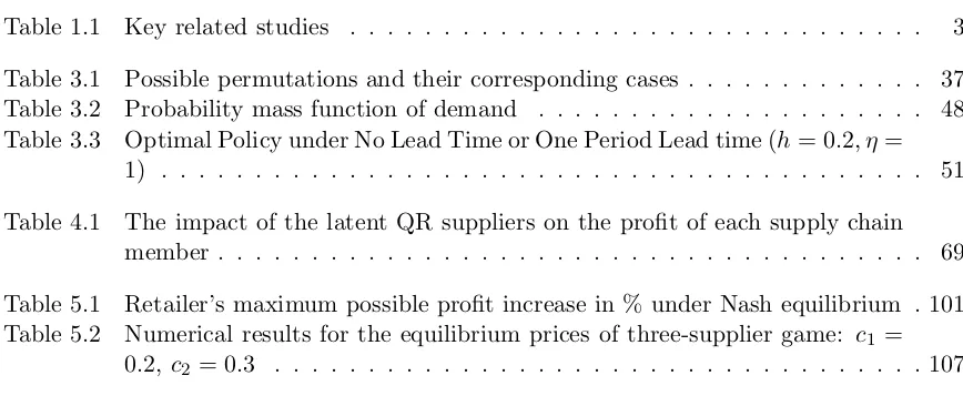
List of Tables . . . .viii
List of Figures . . . ix
Chapter 1 Introduction . . . 1
Chapter 2 Literature Review . . . 8
2.1 Game Theory in Supply Chain Management . . . 8
2.2 Quick Response Supply Chain . . . 10
2.3 Supply Disruption . . . 13
2.4 Supplier Pricing . . . 15
2.5 Bounded Rationality in Supply Chain Management . . . 16
Chapter 3 Optimal Policy for a Dual-Supplier System under Disruption . . . 18
3.1 Introduction . . . 18
3.2 A Finite Horizon Model . . . 23
3.3 An (s, S)-like Optimal Ordering Policy . . . 28
3.4 Extension to an Infinite Horizon Model . . . 40
3.5 Numerical Studies . . . 45
3.6 Concluding Remarks . . . 52
Chapter 4 A Quick Response Supply Chain with Endogenous Wholesale Prices 54 4.1 Introduction . . . 54
4.2 Model and Assumptions . . . 57
4.3 Results with Exponential Demand . . . 61
4.3.1 Single Sourcing . . . 61
4.3.2 Dual Sourcing . . . 63
4.3.3 Preferred Sourcing Strategy of Each Supply Chain Member . . . 64
4.4 Effects of Adding Additional QR Suppliers . . . 67
4.5 Generalization of Results . . . 71
4.5.1 Single Sourcing . . . 71
4.5.2 Dual Sourcing . . . 73
4.5.3 Retailer’s Preferred Sourcing Strategy . . . 78
4.6 Concluding Remarks . . . 80
Chapter 5 Pricing Game with a Bounded Rational Retailer . . . 82
5.1 Introduction . . . 82
5.2 The Model . . . 86
5.3 Best Response Analysis . . . 90
5.4 Nash Equilibrium Analysis . . . 96
5.5 Extensions . . . 104
5.5.2 Numerical Results for the 3-Supplier Case . . . 107
5.5.3 2-Suppliers with a No-Purchase Option . . . 108
5.6 Concluding Remarks . . . 110
Chapter 6 Conclusions. . . .113
6.1 Summary and Contributions . . . 113
6.2 Future Research . . . 115
References. . . .118
APPENDICES . . . .128
Appendix A Appendix for Chapter 3 . . . 129
A.1 (s, S) Policy . . . 129
A.2 The Impact of Beta . . . 131
Appendix B Appendix for Chapter 4 . . . 138
LIST OF TABLES
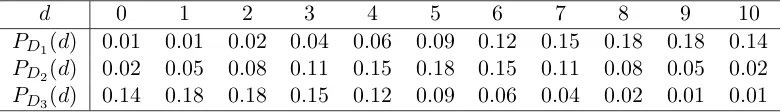
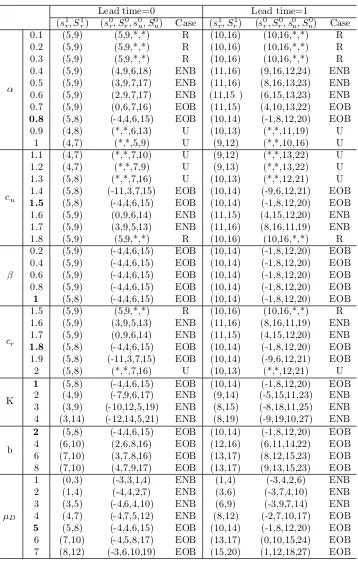
Table 1.1 Key related studies . . . 3 Table 3.1 Possible permutations and their corresponding cases . . . 37 Table 3.2 Probability mass function of demand . . . 48 Table 3.3 Optimal Policy under No Lead Time or One Period Lead time (h= 0.2, η =
1) . . . 51 Table 4.1 The impact of the latent QR suppliers on the profit of each supply chain
member . . . 69 Table 5.1 Retailer’s maximum possible profit increase in % under Nash equilibrium . 101 Table 5.2 Numerical results for the equilibrium prices of three-supplier game: c1 =
0.2,c2= 0.3 . . . 107
LIST OF FIGURES
Figure 3.1 Timeline for one period . . . 24
Figure 3.2 Minimum of mr t(yr) may not exist1 . . . 35
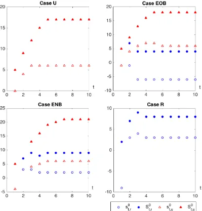
Figure 3.3 Optimal policy over the time as α changes . . . 47
Figure 3.4 Optimal policy over the time as cu changes . . . 47
Figure 3.5 Convergence of (s, S) values under all four cases . . . 49
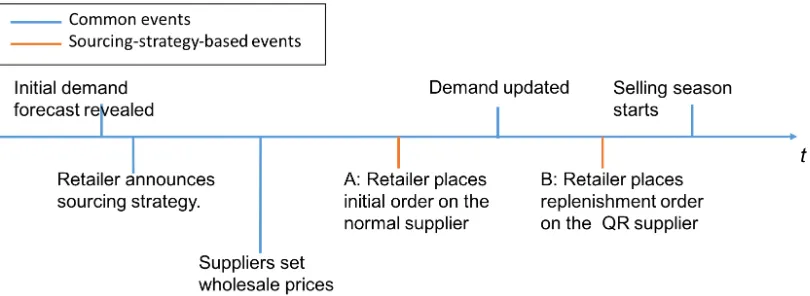
Figure 4.1 The sequence of events in time . . . 59
Figure 4.2 Equilibrium under single sourcing . . . 62
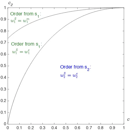
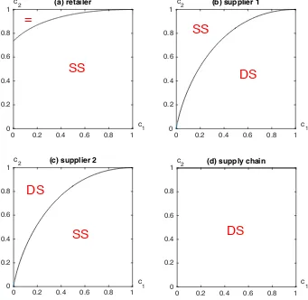
Figure 4.3 Preferred sourcing strategy for each supply chain member over different c1,c2(“SS”:single sourcing, “DS”:dual sourcing, “=”: indifferent between the two sourcing strategies) . . . 67
Figure 4.4 Direction of supply chain profit change under dual sourcing with latent QR suppliers . . . 70
Figure 4.5 Nash equilibrium may (a) or may not (b) exist . . . 76
Figure 5.1 The supplier’s expected profit as a function of his wholesale prices under different β when the competitor’s price is known: wj = 0.8 . . . 91
Figure 5.2 Supplier’s best pricing under different β given wj . . . 92
Figure 5.3 Supplier’s best pricing as wj varies . . . 93
Figure 5.4 Profit loss as a function of β if bounded rationality is ignored . . . 96
Figure 5.5 Profit loss as a function of wj if bounded rationality is ignored . . . 96
Figure 5.6 Nash equilibrium of supplier pricing game . . . 98
Figure 5.7 Profit under equilibrium with different levels of bounded rationality and profit when bounded rationality is ignored by suppliers . . . 102
Figure 5.8 Equilibrium price trajectory as bounded rationality level increases: with-out (blue) and with (red) the no-purchase option . . . 110
Figure A.1 The impact ofβ on optimal policy: asα varies . . . 132
Figure A.2 The impact ofβ on optimal policy: ascu varies . . . 133
Figure A.3 The impact ofβ on optimal policy: ascr varies . . . 134
Figure A.4 The impact ofβ on optimal policy: ash varies . . . 135
Figure A.5 The impact ofβ on optimal policy: asb varies . . . 136
Figure A.6 The impact ofβ on optimal policy: asK varies . . . 137
Chapter 1
Introduction
Supply chains, whether in the manufacturing or service sector, usually consist of players be-longing to different companies with conflicting objectives. Optimizing for a single firm and failing to account for interactive strategic relationships among supply chain members usually results in skewed perspectives. In this dissertation, we concentrate on a two-echelon supply chain consisting of one retailer and multiple suppliers. This two-echelon supply chain is able to capture some features of the reality, yet remains amenable to theoretical analysis. We focus our interest on the retailer’s ordering strategy, the suppliers’ pricing decisions, and the performance of the supply chain as a whole. This dissertation is comprised of three essays, each looking into a supply chain with a different feature. Taking into account strategic planning of different supply chain members, we uncover unexpected managerial insights that would otherwise remain hidden.
production. Given this, many firms still maintain more costly domestic production facilities in order to better respond to any changes in the supply process and uncertainties in the customer demand. Firms need to determine the order allocation among different supply sources based on purchasing price, reliability, inventory status and the available forecast of market demand. The investment U.S. retailers spend on merchandise and service procurement is enormous. To maintain their competitive advantage, it is very important for firms to remain open to potential outsourcing opportunities and design more innovative and holistic sourcing strategies. These issues raise the need to study the retailer’s ordering strategy in face of multiple suppliers.
policy is optimal under a wide range of system parameters beyond the conditions required in the optimality proof. We provide managerial insights into questions such as how the retailer should determine whether to adopt a single or multiple sourcing strategy; how much to order from each supplier; and how to respond to the changes in reliability level and purchase costs.
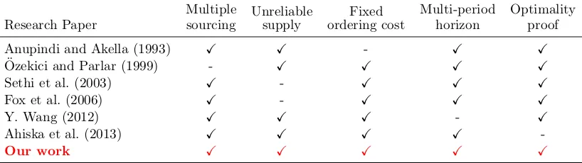
Table 1.1 summarizes some selective studies that are most related to our work. To the best of our knowledge, this is the first study that examines the optimality of a dynamic inventory management policy in a multi-period horizon, where there are two suppliers with unreliable behavior, and a fixed ordering cost is charged.
Table 1.1: Key related studies
Research Paper
Multiple sourcing
Unreliable supply
Fixed ordering cost
Multi-period horizon
Optimality proof
Anupindi and Akella (1993) X X - X X
¨
Ozekici and Parlar (1999) - X X X X
Sethi et al. (2003) X - X X X
Fox et al. (2006) X - X X X
Y. Wang (2012) X X X - X
Ahiska et al. (2013) X X X X
-Our work X X X X X
diversification and price competition effects. Observing two conflicting effects, we are interested in determining which effect takes a dominating role in what scenarios. Therefore, we set out to study a quick response (QR) supply chain, where suppliers make pricing decisions and the retailer decides the order quantity based on suppliers’ quoted prices.
The supply chain we consider in the second essay consists of one retailer and multiple suppliers, similar to our first analysis. In this follow-on study, however, all suppliers are perfectly reliable but vary in their lead times. The suppliers come in two types: the normal supplier and the QR supplier. The normal supplier has a longer lead time compared with the QR supplier. The short lead time of the QR supplier allows the retailer to postpone the ordering decision until more information on market demand is collected. Hence, by ordering from the QR supplier, the retailer is able to reduce demand mismatch costs, i.e., the overage cost when there is any excessive inventory and the stock-out cost when there is any unmet demand. The retailer faces the trade-off between a more accurate demand forecast enabled by shorter lead time and a less expensive ordering cost. We shed light on how the retailer should balance between the initial order and the expedited order. In addition, this work goes one step further to investigate the behavior of the suppliers by allowing the suppliers to set their wholesale prices. When the suppliers are exogenous, it is generally believed that the firms benefit from seeking more flexibility and responsiveness. The involvement of supplier wholesale price setting accounts for the interactive relationship between the retailer and the suppliers and, consequently, can help generate insights that may have been overlooked and explain some seemingly implausible results.
additional QR suppliers affects only the incumbent QR supplier and the retailer, with the QR supplier impaired and the retailer benefited; the normal supplier and the whole supply chain are unaffected. Under dual sourcing, the retailer enjoys higher profit, and both the normal supplier and the QR supplier suffer from the intensified competition; however, the impact on the supply chain depends on the suppliers’ production costs. We find that additional QR suppliers can be advantageous to the supply chain under dual sourcing when the cost of the critical additional QR supplier is not significantly higher than that of the normal supplier.
information collection and/or limited information processing. Generally, this set of behavioral phenomena is called bounded rationality in the literature. Scholars believe that as a new tool, bounded rationality has tremendous potential to generate novel research problems and provide a fresh perspective to provide new insights to mainstream operations management problems (Shen & Su, 2007). Hence, we set out to examine the supplier pricing game through the lens of bounded rationality.
the supplier who provides a price cut is the cost-efficient supplier, from whom the retailer is more likely to make an order. Consequently, the price reduction from the cost-efficient supplier is directly reflected in the retailer’s revenue, and the retailer earns a higher profit when she deviates from perfect rationality. We have also investigated the impact of bounded rationality on the revenue of the retailer and each supplier, as well as the social welfare of the supply chain. This essay provides a fresh perspective on supplier pricing decisions by taking into consid-eration human behavior and emotions when facing difficult decision problems. Our analysis suggests that, contrary to conventional wisdom, whereby bounded rationality is always con-sidered to be a performance-degrading impediment, the retailer can actually benefit from her bounded rationality. Thus, the retailer does not have to strive for perfect rationality, and more-over, she could endeavor to project on the suppliers an image of an incomplete rationality. We hope this study enlightens our views on bounded rationality, and in doing so, stimulates future research on behavioral theory in supply chain management.
Chapter 2
Literature Review
Snyder and Shen (2011) and Zipkin (2000) provide a broad overview of interesting topics in supply chain management. In this dissertation research, we are particularly interested in certain methodologies applied in supply chain management (e.g., game theory), certain types of supply chain (e.g., a supply chain with quick response capability and a supply chain subject to supply disruption), certain problems in supply chain management (e.g., supplier pricing problem), and certain characteristics of supply chain participants (e.g., the supply chain members are not perfectly rational). In this chapter, we review these topics that are closely related to this dissertation.
2.1
Game Theory in Supply Chain Management
It is not unusual in the supply chain management that the profit of a corporation is affected by the competing corporations or by the upstream suppliers. Game theory is an effective tool for analyzing the situations when the profit of an agent is affected by the decisions of other agents. As such, game theory studies the interaction of decision makers.
is widely employed to characterize a stable outcome, where no player will unilaterally deviate because such a behavior will result in a lower payoff. However, the cooperative game focuses on the behavior of groups of players, associating the action and payoff to every group, and seeks to find the stable coalition, i.e., groups of people, that will be formed. The concept of the core is applied to refer to a payoff allocation of the grand coalition such that there does not exist a coalition of players that could make all of its members at least as well off. The last twenty decades have witnessed a successful application of non-cooperative game in the field of supply chain management. An excellent review can be found in Cachon and Netessine (2004). Papers that adopt a cooperative game approach are relatively scant, but are becoming more prevalent. This emergence is probably due to the increasing prevalence of bargaining and negotiation in the supply chain. Nagarajan and Soˇsi´c (2008) provide a detailed survey of the existing literature on the cooperative game in supply chain analysis.
studies on inventory competition can be found in Mahajan and Van Ryzin (2001), Netessine and Rudi (2003) and Caro and Mart´ınez-de Alb´eniz (2010). Pricing competition is another main stream in the literature. J. Li et al. (2010) study a single-retailer-two-supplier supply chain in which the suppliers compete for the retailer order by setting their wholesale prices. Dai et al. (2005) examine the retailers’ pricing strategies to attract customer orders under capacity constraints. Cai et al. (2009) focus on the pricing competition between the traditional retailer channel and the online direct channel and evaluate the impact of different pricing strategies.
When the players take actions sequentially, a Stackelberg game is applied and the subgame perfect Nash equilibrium (SPNE) is of great significance. In the supply chain management, the interaction between the supplier and the retailer is often modeled by a Stackelberg game. In such a game, the supplier traditionally acts as a leader, setting the wholesale price or other contract parameters, and the retailer acts as a follower, making ordering decision and sometimes setting retail price. Lariviere and Porteus (2001) study a game between the supplier and the retailer where the supplier sets the wholesale price and then the retailer makes the ordering decision based on the quoted wholesale price. An example of a Stackelberg game with the supplier choosing the stocking inventory and the retailer deciding on promotional effort level can be found in Netessine and Rudi (2004). See Lin and Parlakt¨urk (2012) for a Stackelberg game in the QR supply chain where the supplier sets the wholesale price and then the competing retailers place the regular orders and QR orders sequentially.
2.2
Quick Response Supply Chain
to a fashion ski-wear firm and creates a profit of 60% compared to the existing inventory system. Eppen and Iyer (1997) examine an inventory model where dumping inventory to outlet stores is allowed. They provide an updated newsboy heuristic algorithm when the purchasing decision is only available at the beginning of the first period and the dumping decision can be made at the beginning of each period. Gurnani and Tang (1999) consider a retailer with two ordering instants before the selling season; however, the unit purchasing cost at the second instant is uncertain. They propose a nested newsvendor model for determining the optimal order quantity, discuss the value of information and provide suggestions to the retailer when to postpone the ordering decision. Choi et al. (2003) extend the cost uncertainty form to a general discrete distribution and characterize the optimal ordering policy using dynamic optimization. Fisher et al. (2001) propose a heuristic algorithm to determine the optimal initial and replenish order for a catalog retailer. Their method can also be used to optimize the reorder time and quantify the benefit of lead time reduction. J. Li et al. (2009) examine a similar framework of Fisher et al. (2001), but utilize a quite different approach. Instead of making suggestions on the optimal ordering level, J. Li et al. (2009) shed light on the optimal policy structure for three interacted decisions: the first order quantity, the timing of second order and the second order quantity. The conditions for the problem to be well-behaved is also established. Lau and Lau (1997) also consider a retailer with mid-season replenishment and develop a solution procedure in case of normal demand distribution. Fu et al. (2013) and Choi et al. (2004) consider a retailer having multiple options of expedition and facing the trade-off between cost and responsiveness. Under a Bayesian model of demand update mechanism, Milner and Kouvelis (2002) further examine the best timing of the second order. Several scenarios (demand level, lead time length, demand uncertainty level) are discussed to evaluate the value of information and production timing flexibility. Milner and Kouvelis (2005) study how the value of production quantity flexibility and production timing flexibility is affected by product demand characteristics.
relation-ship between the supplier and the retailer. Iyer and Bergen (1997) study the impact of QR on a two-tier supply system and find that QR benefits the retailer but can be detrimental to the supplier. They further design several contracts such as higher service levels, wholesale price and volume commitments so as to make QR a Pareto improving strategy. Donohue (2000) considers a two-stage newsvendor model with a general demand update rule, and proposes a buyback contract that motivates the retailer to order at a level that coordinates the supply chain. Lariviere and Porteus (2001) consider a manufacturer selling to a newsvendor and de-velop the regularity conditions, satisfied by many common distributions, for the manufacturer’s decision to be analytically tractable. Weng (2004) examines a QR supply system consisting of one manufacturer and one retailer, where the manufacturer can dictate its wholesale prices. Their focus is channel coordination and a quantity discount policy is proposed to induce the buyer to order the coordinated quantity. Cachon and Swinney (2011) study the interaction between the retailer and the consumers: Consumers decide whether to buy now or wait for the clearance, based on the regular price and their conjecture on the discounted price and the possibility their desired item will last to the clearance. They show that QR helps blunt con-sumers’ strategic behavior of intentionally waiting for markdowns, because the retailers with QR capability are able to reduce excessive inventory left and therefore reduce the occurrence of markdowns.
Zip-(1994) innovate a general probabilistic model of demand evolution process, i.e., the Martingale model of forecast evolution (MMFE). The time series approach assumes that demand follows some classical time series (e.g., auto-regressive moving-average process) in which correlation exists among consecutive demand realizations; see Veinott Jr (1965), Johnson and Thompson (1975), and Aviv (2003).
2.3
Supply Disruption
The disruptions in supply process can be attributed to natural factors (such as earthquakes, floods, storms, etc) and intentional or unintentional human actions (such as machine break-downs, strikes, financial defaults, etc). Recently, an increasing number of scholars have shifted their attention to the randomness in the supply process, resulting in the proliferation of pub-lications. Snyder et al. (2012) provide a comprehensive review of OR/MS models for supply chain disruption.
In the literature, models of uncertainties in supply process can be divided into the fol-lowing four categories: random yield, all-or-nothing delivery, random lead times and supplier unavailability.
Random yield assumes only a portion of the order is received or a fraction of the order is defective. I refer the readers to Yano and Lee (1995) for a comprehensive review of supply uncertainty with random yield. Federgruen and Yang (2009) analyze a supplier selection and order allocation problem given the set of potential suppliers with random yield factor with a general probability distribution. Two approximation algorithms, based on large-deviations technique and central limit theorem, respectively, are developed, and their asymptotic behaviors are analyzed. Gurnani et al. (2000) consider an assembly system using two components subject to production yield losses, and study the combined ordering and assembly decisions.
fixed cost, an environment-dependent (s, S) policy is shown to be optimal. Model I of Anupindi and Akella (1993) considers a retailer facing a continuous random demand and procuring from two uncertain suppliers with all-or-nothing delivery. It is shown that the optimal ordering policy is no other than three cases: order nothing, order from the less reliable supplier with a lower cost, order from both suppliers. Swaminathan and Shanthikumar (1999) study the same problem but consider discrete demand distribution, and find a different result: ordering solely from the more reliable but more expensive supplier can be optimal under some cases. Babich et al. (2007) study the scenario when the suppliers’ disruption are correlated and allow the suppliers to control their wholesale prices.
Lead time uncertainty is characterized by a random lead time distribution. Model III of Anupindi and Akella (1993) considers delayed delivery as a special form of lead time uncertainty by assuming that the orders not successfully delivered by the unreliable supplier in the current period will definitely arrive in the next period. More discussion on lead time uncertainty can be found in Bagchi et al. (1986), Song (1994) , and Y. Wang and Tomlin (2009).
For supplier unavailability, the supplier’s status can go from up to down time to time and orders placed when the supplier is down cannot be delivered successfully. Parlar and Perry (1996) analyze two identical unreliable suppliers in a continuous-review context, where the durations of up/down periods are exponentially distributed. G¨urler and Parlar (1997) extend the work of Parlar and Perry (1996) by considering Erlang-kdistributed availability durations and general unavailability durations.
2.4
Supplier Pricing
In many literatures, it is assumed that the wholesale price that the retailer pays to the supplier for each unit of product purchased is exogenous. Supplier pricing allows the supplier to set the wholesale price and accounts for the interactive relationship between the retailer and the supplier. In the one-supplier-one-retailer supply chains, most of the research that allows for supplier pricing is devoted to designing and constructing different classes of pricing policies, i.e., contracts, to mitigate the double marginalization that leads to supply chain inefficiency. We refer the readers to surveys by Anupindi and Bassok (1999), Lariviere (1999) and Cachon (2003).
the same spirit, Calvo and Mart´ınez-de Alb´eniz (2015) study a retailer sourcing potentially from one normal supplier and one QR supplier, and shows that different from general wisdom, the retailer would prefer single sourcing to dual sourcing when the suppliers take pricing decisions.
2.5
Bounded Rationality in Supply Chain Management
As demonstrated by empirical experiments, human decision makers do not necessarily make the best choice as theory suggests. In fact, people intend to be rational, but due to cognitive constraint or limited information, they fail in the decision making process. Bounded rationality provides a notion that the decision maker may not be perfectly rational to make the choice that yields the highest level of benefits.
The seminal work of Simon (1955) suggests that instead of performing an exhaustive search, the decision maker will settle for something satisfactory, but less than perfect. Rubinstein (1998) surveys the cognitive limitation that leads to the inherent imperfection of human decision making. Another stream of research has focused on heuristics or rule of thumb (see, e.g., Tversky & Kahneman, 1974), which navigates people in complex decision making process. The review on evolution and development of bounded rationality can be found in Conlisk (1996) and Simon (1982). Boudreau et al. (2003), Bendoly et al. (2006), Loch and Wu (2007), and Gino and Pisano (2008) provide good surveys on behavioral issues in operation management.
derived by theoretical results. Su (2008) suggests that such behavior can be explained by incorporating “noise” into the newsvendor’s decision process, such that the optimal solution is stochastically preferred by the newsvendor, but not in a deterministic manner. Schweitzer and Cachon (2000) are inclined to the explanation that the newsvendors gain some utility from reducing the left-over inventory, and they anchor their decisions upon the demand average and do not adjust sufficiently towards the optimal ordering quantity.
Prospect theory represents another main stream of modeling bounded rationality in supply chain management. According to prospect theory, the decision maker subconsciously forms a reference point and measures the loss more significantly compared with the same magnitude of gain. As such, prospect theory suggests that utility not only generates from accumulating wealth, but also from losing and gaining wealth. C. X. Wang and Webster (2009) examine a risk-averse newsvendor and find that the he/she will order more (less) than a risk-neutral newsvendor when the shortage cost is high (low). An inventory management with two suppliers under supply disruption is studied through a prospect theory lens by Giri (2011). Ma et al. (2012) analyze a QR supply chain with two ordering opportunities and information updates when the buyer is loss-averse. See Wu et al. (2010) for the impact of risk-aversion on manufacturer’s optimal policy in supply contracts. Popescu and Wu (2007) study a dynamic pricing problem when consumer demand is dependent on the pricing history. Prospect theory reflects in how the consumers perceive gains and losses relative to previous prices.
Chapter 3
Optimal Policy for a Dual-Supplier
System under Disruption
3.1
Introduction
philos-supply disruption. Additionally, as companies outsource a greater proportion of their manufac-tured products from low-cost countries that are politically and economically less stable, they become more prone to disruptions.
To mitigate the negative effects of supply disruptions, the simultaneous involvement of two sources in geographically different locations may turn out to be more economical. Some companies employ a form of dual sourcing such that the firm sources exclusively from one supplier when that supplier is available but reroutes to the backup supplier during disruptions (Tomlin, 2006). In addition to providing a back-up source in case of emergency, multiple sourcing is favored by firms for a variety of strategic reasons, such as maintaining competition or meeting customer volume requirements. In particular, a small base of two or three suppliers is favored by firms to reap the benefits of both single sourcing and multiple sourcing yet avoid the disadvantages of purely single sourcing. The selection of suppliers and the optimal size of the supply base is not the emphasis of this work. Instead we are interested in providing insight into the optimal sourcing strategy given a set of two suppliers with different costs and disruption probabilities. Research questions emerge when a supplier, who operates at a high reliability level, but has cost. Sourcing solely from this premium supply agent is expensive and often a non-optimal strategy. On the other hand, due to supply interruptions, purchasing exclusively from the less expensive supplier can likewise be costly.
assumed that the order is either delivered in full or it is canceled depending on its status. This all-or-nothing delivery is valid when, for example, there is a quality problem in production, the production process is interdicted by strike, products are destroyed entirely by fire, or perishable goods deteriorate. The unreliable supplier does not accept any orders when it is down. The supply availability at the beginning of the period does not imply the successful delivery of the products since the state of the unreliable supplier can change from up to down after the order has been made. In this case, the entire order is canceled. Fixed ordering cost is incurred when an order is placed, regardless of whether the order is delivered or not. Unit purchase cost is charged only for the order that is actually delivered.
In this chapter, we first consider a finite-horizon model, where dynamic programming (DP) techniques are used to find the optimal rule for selecting the order quantity for each period given any possible initial inventory level and supply availability status. We apply the concept of K-convexity to prove that the optimal policy has an (s, S)-like structure. Under an (s, S) policy, an order is placed to raise the inventory level to S when the inventory level reaches or drops below s. We start with the analysis of a single period model and demonstrate by mathematical induction that under certain technical conditions, the (s, S)-like policy remains optimal for any finite-horizon model. We further refine the proposed (s, S)-like policy into four cases depending on the order of the indebted s, S values. The four cases are referred to as
• Case U: order exclusively from the unreliable supplier;
• Case EOB (either or both): either order from both suppliers or order from the unreliable supplier depending on the inventory level;
• Case ENB (either, not both): order from either the reliable supplier or from the unreliable supplier, but not both, based on the inventory level;
unit cost increases, or backorder cost reduces, the optimal case evolves from Case R to Case ENB to Case EOB, and finally to Case U. Particularly, we are able to distinguish Case U from the remaining cases by a simple computation on the parameters. Next, we extend to an infinite-horizon setting and verify the convergence of the total optimal cost. The convergence of the optimal policy follows from the convergence of the optimal cost, and the resulting limiting policy serves as the optimal ordering policy for the infinite-horizon framework. Characterization of the optimal policy is important because it confines the optimal policy to a certain boundary that facilitates the designing of either exact or heuristic algorithms. In light of the previous literature that focuses on inventory problems that exhibit an (s, S) policy, this is, to the best of our knowledge, the first paper that provides theoretical proof on the optimality of (s, S)-like policy for a multi-period inventory system with two suppliers under supply disruption.
and verifies the optimality of a generalized (s, S) policy through introducing the quasi-K-convex function. Instead of considering the demand as a pure random variable (most models consider an i.i.d. distribution), Sethi and Cheng (1997) assume that the demand distribution is dependent on a Markov chain, and show that the optimal policy is a state dependent (s, S) policy when there is a fixed ordering cost.
One common strategy to mitigate the negative effects of uncertainty in the supply system is to order from multiple suppliers. The literature on multiple sourcing has focused on the selection of suppliers and determination of order quantity from each supplier. Dada et al. (2007) consider the selection of unreliable suppliers in a newsvendor setting. Dual sourcing is particularly important because it preserves the advantage of single sourcing and greatly reduces risks. Fox et al. (2006) consider trade-offs between a supplier with a lower variable cost but nonzero fixed cost and a supplier with high variable cost and negligible fixed cost. The resulting optimal policy can be generalized into three cases: a base-stock policy for ordering from the high variable cost supplier, an (sLV C, SLV C) policy for purchasing exclusively from the low variable cost supplier and a hybrid (s, SHV C, SLV C) policy for buying from both suppliers. The result holds for both lost sales and back-order cases. Sethi et al. (2003) consider an inventory system with fast and slow delivery modes (the fast mode is assumed to be more expensive than the slow mode). With the existence of fixed ordering cost and demand information update, a forecast-update-dependent (s, S) type policy is proved to be optimal. However, there is no unreliability issue addressed in the above literature.
Y. Wang (2012) investigates the optimal policy of ordering from two unreliable suppliers. Taking into account different configurations of the fixed ordering cost including overall, placement and receipt costs, Wang develops the characteristics of optimal policy and its dependence on system parameters. However, only single-period problems are discussed. Ahiska et al. (2013) analyze an inventory model in which a retailer replenishes from one reliable supplier and one unreliable supplier. Through abundant numerical experiments solved by a corresponding Markov Decision Process (MDP), they report that the optimal policy appears to be an (s, S) policy when the unreliable supplier is down, and generalize the policy into four cases when the unreliable supplier is up, depending upon problem parameters.
The rest of this chapter is organized as follows: We state our model, list the notation and provide definitions in§3.2, and prove the optimality of (s, S)-like ordering policy under a finite horizon framework in §3.3. An extension to the infinite horizon scenario is studied and the convergence of the optimal cost function and the optimal policy is presented in §3.4. In §3.5, through computational experiments, the optimality of the proposed policy is verified for a range of cost configurations and different supply reliability levels. Conclusions are provided in§3.6.
3.2
A Finite Horizon Model
be placed on the unreliable supplier when it is down at the beginning of the period. In this case, the only option for the retailer is to order from the reliable supplier. Even if the unreliable supplier is up at the beginning of the period, it does not guarantee that the placed order will be successfully delivered. It is possible that the unreliable supplier goes from up to down after the order is placed, and consequently, the active order is canceled. The retailer needs to decide, based on its inventory level, how much to order and how to distribute the order.
Fixed ordering cost, assumed to be the overhead cost of generating an order, is considered. For each supplier, if an order is placed, a fixed ordering cost is charged whether the order is delivered or not. Unit ordering cost, assumed to be linear in the order quantity, is incurred for the products that are finally received. A unit holding cost is incurred for each unit held in stock at the end of a period. There is a unit penalty cost when the retailer does not have enough inventory to satisfy the demand. It is assumed that fulfilled orders from both suppliers arrive before demand is realized. The retailer fulfills its stochastic demand from the market with on-hand inventory and backlogs any unsatisfied demand. The events in each period are shown in Figure 3.1. Since we consider a finite-horizon model, the overall schedule repeats the daily events.
State of the system (X,J) observed; ordering decisions
qrandquare made
Holding and back-ordering cost calculated Orders arrive
Status of the unreliable supplier may change
Demand is realized Period𝑡
The following notation is introduced:
qr : order quantity on the reliable supplier; qu : order quantity on the unreliable supplier; cr : unit ordering cost of the reliable supplier; cu : unit ordering cost of the unreliable supplier; Kr : fixed ordering cost of the reliable supplier; Ku : fixed ordering cost of the unreliable supplier;
α: probability that the unreliable supplier remains up in the next period when its current state is up, 0< α <1;
β : probability that the unreliable supplier becomes up in the next period when its current state is down, 0< β≤1;
W :
0 1
0 1
α 1−α β 1−β
, transition probability matrix for the status of the unreliable
sup-plier, where state 0 is the up state and state 1 is the down state; b: backorder cost per item per period,b≥cr;
h: holding cost per item per period;
D: demand distribution, with f(·) being its pdf and F(·) being its cdf;
ED[·] : expected value w.r.tD; and η : period discount factor, 0< η≤1.
recovery probability. The assumption b≥cr is made to avoid trivial cases.
The problem can be formulated as a stochastic dynamic programming (DP). The state of the system is characterized as the tuple (X,J), whereX is the initial inventory at the beginning of each period andJ is the state of the unreliable supplier (0-up, 1-down). The retailer’s inventory level is limited to a range [Imin, Imax], whereImaxrepresents the storage capacity of the retailer and Imin may be a negative number, indicating the maximum backorder level allowed by the retailer. These limits on the range of the inventory level can be set arbitrarily large (positively or negatively) to reflect unlimited inventory or backorders yet restrict the number of states such that the problem is not excessively difficult computationally. Let θjt(x) denote the total discounted cost of operatingt periods when the optimal policy is implemented in each period, given X = x and the unreliabler’s status J = j. The optimal discounted cost of a t-period problem when the unreliable supplier is up becomes
θ0t(x) = min
qu>0 qr>0
{Krδ(qr) +Kuδ(qu) +crqr+αcuqu+αg(x+qr+qu) + (1−α)g(x+qr)
+αηED[θ0t−1(x+qr+qu−D)] + (1−α)ηED[θt1−1(x+qr−D)]}, (3.1)
and the corresponding cost when the unreliable supplier is down becomes
θ1t(x) = min qr>0
{Krδ(qr) +crqr+g(x+qr) +βηED[θ0t−1(x+qr−D)]
+ (1−β)ηED[θ1t−1(x+qr−D)]}, (3.2)
whereg(·) is theloss function, defined below as the sum of inventory cost and backorder cost:
g(y) =h
Z y
0
(y−ξ)f(ξ)dξ+b
Z ∞
y
δ(x) is defined over [0,∞) as δ(x) =
0 ifx= 0 1 ifx >0
. When t = 1, there is no future cost, so we arbitrarily assume there is not salvage value for residual inventory and so we define θj0(x) = 0,∀x∈[Imin, Imax], j ∈ {0,1}.
At the beginning of each period, the retailer observes its inventory level and must decide the amount to order from each supplier. Instead of using the order quantities qr and qu, it is convenient to recast the decision variables to order-up-to levels yr and yu. In practice, the orders on the two suppliers are placed simultaneously. However, for analytical tractability, we consider first ordering from the reliable supplier and so defineyras the inventory position after ordering from the reliable supplier and yu as the inventory position after ordering from the unreliable supplier under the assumption that the order is delivered successfully. Given the inventory level at the beginning of the periodX =x, the following relationship between order quantities and order-up-to levels holds:
yr=x+qr, yu=x+qr+qu.
The cost function can be reformulated as
θ0t(x) = min
yu>yr yr>x
{Krδ(yr−x) +Kuδ(yu−yr) +cryr+αcu(yu−yr) +αg(yu)
+ (1−α)g(yr) +αηED[θ0t−1(yu−D)] + (1−α)ηED[θ1t−1(yr−D)]} −crx; (3.3)
θ1t(x) = min yr>x
{Krδ(yr−x) +cryr+g(yr) +βηED[θt0−1(yr−D)]
+ (1−β)ηED[θ1t−1(yr−D)]} −crx. (3.4)
3.3
An
(s, S
)
-like Optimal Ordering Policy
In this section, we propose an (s, S)-like policy as follows: when the unreliable supplier is up, order first from the reliable supplier according to an (s0r, Sr0) policy and then order from the unreliable supplier according to an (s0u, Su0) policy, henceforth referred to as an (s0r, Sr0, s0u, S0u) policy; moreover, when the unreliable supplier is down, order from the reliable supplier based on an (s1r, Sr1) policy. Optimality of this policy is proven by mathematical induction. We start with a single period case and show the optimal policy in Lemma 3.3.1. Then, for any finite horizon of more than one period, the optimality of an (s1
r, Sr1) policy when the unreliable supplier is down and an optimal (s0r, Sr0, s0u, Su0) policy when the unreliable supplier is up are addressed in Lemma 3.3.2 and Lemma 3.3.3, respectively. Furthermore, we obtain the condition when s0r and Sr0 do not exist, as presented in Proposition 3.3.4.
To make the objective analytically tractable, we rewrite Eq. (3.3), which is the cost function of tperiods when the unreliable supplier is available, as
θ0t(x) = min yr>x
{Krδ(yr−x) + (cr−αcu)yr+ (1−α)g(yr) + (1−α)ηED[θt1−1(yr−D)] + min
yu>yr
{Kuδ(yu−yr) +αcuyu+αg(yu) +αηED[θt0−1(yu−D)]}} −crx. (3.5)
For ease of representation, we define the following expressions:
mut(yu) =αcuyu+αg(yu) +αηED[θ0t−1(yu−D)]; (3.6) Lt(yr) = min
yu>yr
{Kuδ(yu−yr) +mut(yu)}; (3.7)
mrt(yr) = (cr−αcu)yr+ (1−α)g(yr) + (1−α)ηED[θ1t−1(yr−D)] +Lt(yr). (3.8)
Thus, the dynamic cost function can be rewritten as
θ0t(x) = min yr>x
{Krδ(yr−x) +mrt(yr)} −crx, (3.10) θ1t(x) = min
yr>x
{Krδ(yr−x) +m1t(yr)} −crx. (3.11)
Letx be the inventory level at the beginning of a period and denote ˜yt,r0 (x) and ˜yt,u0 (x) as the functions that minimize (3.3), and ˜y1t,r(x) as the function that minimizes (3.4). We are now ready to analyze the optimal policies in each period.
Lemma 3.3.1. In a single period model, if g(y) is convex and Kr ≥ Ku, then we have the following results:
(i) when the unreliable supplier’s state is down:
˜ y11,r =
S1
1,r, if x6s11,r,
x, otherwise,
(3.12)
withS11,r being the minimizer of m11(yr) and s11,r < S11,r.
(ii) when the unreliable supplier’s state is up:
˜ y10,r =
S10,r, if x6s01,r,
x, otherwise,
if mr1(yr) has a minimum,
x, otherwise,
(3.13)
where S10,r is the minimizer of mr1(yr), if exists and s01,r < S10,r;
˜ y10,u =
S0
1,u, if x6s01,u, ˜
y01,r, otherwise,
(3.14)
where S10,u is the minimizer of mu1(yr) and s01,u< S10,u.
Proof. (i) For a single period model, when the unreliable supplier is down,m11(yr) =cryr+g(yr), and limyr→−∞cryr+g(yr)→ ∞ sinceb > cr. Therefore, according to Lemma A.1.3, if g(y) is
convex, there existss11,r independent ofx such that
θ11(x) = min yr>x
{Krδ(yr−x) +m11(yr)} −crx = min
yr>x
{Krδ(yr−x) +cryr+g(yr)} −crx
=
Kr+crS11,r+g(S11,r)−crx, ifx6s11,r, g(x), ifx > s11,r.
(3.15)
Eq. (3.15) implies that when x 6 s11,r, it is best to order up to S11,r, and when x > s11,r, it is best not to make any order. Hence, Eq. (3.12) follows.
(ii) When the unreliable supplier is up, we have L1(yr)=minyu>yr{Kuδ(yu−yr) +αcuyu+
αg(yu)}. Since αcuyu+αg(yu) is convex and limyu→−∞αcuyu+αg(yu)→ ∞, there exists
0 1,u and S10,u such that
L1(yr) =
Ku+αcuS10,u+αg(S10,u), ifyr6s01,u, αcuyr+αg(yr), ifyr> s01,u.
(3.16)
Hence, we have Eq. (3.14). By Lemma A.1.3, it can be shown thatL1(yr) isKu-convex inyr, so isKr-convex inyr. Combining with the fact that (cr−αcu)yrand (1−α)g(yr) are both convex, we knowmr1(yr) = (cr−αcu)yr+ (1−α)g(yr) +L1(yr) isKr-convex. If limyr→−∞m
r
1(yr)→ ∞, we have
θ10(x) = min yr>x
{Krδ(yr−x) + (cr−αcu)yr+ (1−α)g(yr) +L1(yr)} −crx
=
Kr+ (cr−αcu)S10,r+ (1−α)g(S10,r) +L1(S10,r)−crx, ifx6s01,r, (cr−αcu)x+ (1−α)g(x) +L1(x)−crx, ifx > s01,r.
Otherwise,mr1(yr) does not have a minimum and, consequently,
θ01(x) = (cr−αcu)x+ (1−α)g(x) +L1(x)−crx, ∀x. (3.18)
Eq. (3.17) and Eq. (3.18) directly imply Eq. (3.13).
(iii) Lemma A.1.2 (iv) implies that θ01(x) is Kr-convex by definition. The Kr-convexity of θ11(x) follows the same logic.
Lemma 3.3.2. In the finite horizon model, if θt0−1(x) and θt1−1(x) are both Kr-convex for t= 2,3,· · ·, T, then
(i) there exist numberss1t,r, St,r1 with s1t,r < St,r1 such that
˜ yt,r1 =
St,r1 , if x6s1t,r;
x, otherwise.
(3.19)
(ii) θ1t(x) is Kr-convex.
Proof. (i) Because θt0−1(x) andθt1−1(x) areKr-convex,m1t(yr) =cryr+g(yr) +βηED[θ0t−1(yr−
D)]+(1−β)ηED[θ1t−1(yr−D)] isηKr-convex. Besides, since limyr→−∞m
1
t(yr)>limyr→−∞cryr+
g(yr)→ ∞, we have
θ1t(x) = min yr>x
{Krδ(yr−x) +cryr+g(yr) +βηED[θt0−1(yr−D)] + (1−β)ηED[θ1t−1(yr−D)]} −crx
=
Kr+cr(St,r1 −x) +g(St,r1 ) +βηED[θt0−1(St,r1 −D)]+
(1−β)ηED[θt1−1(St,r1 −D)], ifx6s1t,r, g(x) +βηED[θt0−1(x−D)] + (1−β)ηED[θ1t−1(x−D)], ifx > s1t,r.
(3.20)
Eq. (3.19) can be readily obtained through Eq. (3.20).
Lemma 3.3.3. In the finite horizon model, if θt0−1(x) and θt1−1(x) are both Kr-convex for t= 2,3,· · ·, T, and αηKr≤Ku≤(1−(1−α)η)Kr, then
(i) the following results on y˜t,r0 and y˜0t,u hold:
˜ yt,r0 =
St,r0 , if x6s0t,r,
x, otherwise,
if mrt(yr) has a minimum,
x, otherwise,
(3.21)
where St,r0 is the minimizer of mrt(yr), if exists and s0t,r< S0t,r;
˜ yt,u0 =
St,u0 , if x6s0t,u, ˜
yt,r0 , otherwise,
(3.22)
where St,u0 is the minimizer of mut(yr), and s0t,u< St,u0 .
(ii) θ0t(x) is Kr-convex.
Proof. (i) Whenθ0t−1(x) isKr-convex,mut(yu) =αcuyu+αg(yu) +αηED[θt0−1(yu−D)] isαηKr
-convex. It is not difficult to see thatαcuyu+αg(yu)+αηED[θt0−1(yu−D)]> αcuyu+αg(yu)→ ∞ when yu→ −∞. Therefore, if Ku≥αηKr, there existsSt,u0 > s0t,u>−∞such that
Lt(yr) =
Ku+αcuSt,u0 +αg(St,u0 ) +αηED[θt0−1(St,u0 −D)], ifyr6s0t,u, αcuyr+αg(yr) +αηED[θt0−1(yr−D)], ifyr> s0t,u.
(3.23)
exists or not. If limyr→−∞m
r
t(yr)→ ∞, then
θt0(x) = min yr>x
{Krδ(yr−x) + (cr−αcu)yr+ (1−α)g(yr) + (1−α)ηED[θ1t−1(yr−D)] +Lt(yr)} −crx
=
Kr+ (cr−αcu)St,r0 + (1−α)g(St,r0 ) + (1−α)ηED[θ1t−1(St,r0 −D)]
+Lt(St,r0 )−crx, ifx6s0t,r,
−αcux+ (1−α)g(x) + (1−α)ηED[θt1−1(x−D)] +Lt(x), ifx > s0t,r.
(3.24)
Otherwise limyr→−∞m
r
t(yr)→ −∞, i.e.,mrt(yr) does not have a minimum, resulting in ˜y0t,r=x and
θt0(x) =−αcux+ (1−α)g(x) + (1−α)ηED[θt1−1(x−D)] +Lt(x), ∀x. (3.25) Eq. (3.21) follows from Eq. (3.24) and Eq. (3.25).
(ii) From Lemma A.1.3 we know that θt0(x) is Kr-convex.
The above Lemmas establish the optimality of the proposed (s, S)-like policy. We note that Kr ≥Ku is dominated byαηKr ≤Ku≤(1−(1−α)η)Kr. Therefore, the technical condition αηKr ≤ Ku ≤ (1−(1−α)η)Kr alone guarantees the optimality of (s, S)-like policy in each period. Also notice that when η equals to 1, αηKr ≤ Ku ≤ (1−(1−α)η)Kr is reduced to Ku =αKr, which prescribes a single value ofKu for any givenKr. The constraint is less rigid when η takes a small number and requires Ku ≤Kr only when η equals to 0. This constraint may be restrictive to some extent since the discount factor η usually takes a number close to 1. The reason is that in the above proof, we directly apply the K-convexity properties, such as preservation of K-convexity under linear and expectation operations. However, the lemmas do not fully reveal the characteristics of K-convexity. For example, suppose f1(x) is
K1-convex andf2(x) isK2-convex, thenαf1(x) +βf2(x) is (αK1+βK2)-convex for allα, β ≥0
according to Lemma A.1.2. Whereas, in fact, αf1(x) +βf2(x) is usually Q-convex, for some
optimality of the (s, S)-like policy. However, our results, which do not rely on the demand distribution, provide a sufficient condition for the optimality of the (s, S)-like policy when the retailer faces one reliable supplier and one unreliable supplier with fixed costs. In §3.5, we conduct some computational studies to show that the (s, S)-like policy remains optimal for a wide range of system parameters (including unit cost, fixed ordering cost, backorder cost, reliability levels, etc) and demand distributions.
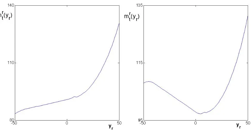
It is noted in Lemma 3.3.3 that mr
t(yr) may not have a minimum. Next, we evaluate the performance of mrt(yr) and discuss when its minimum does not exist. For the classic single supplier problem, mrt(yr) has a minimum when the penalty cost is higher than unit ordering cost(b > c). Otherwise when b ≤ c, instead of paying the unit cost, the retailer always prefers not to purchase and pay the penalty cost. For this two-supplier problem, the same logic applies when later making orders on the unreliable supplier. It does not make a difference when multiplying by a positive number α (see mut(yu)). Therefore, it is guaranteed that limyu→−∞m
u
t(yu) → ∞. However, the situation becomes different when analyzing the order quantity from the reliable supplier, because the minimum of mr
t(yr) may not exist and this happens when limyr→−∞m
r
Figure 3.2: Minimum ofmr
t(yr) may not exist1
Proposition 3.3.4. mrt(yr) does not have a minimum if and only if α≥ bb++ηcηcrr−−ccru.
Proof. The existence of the minimum of mr
t(yr) depends on the slope when yr → −∞, and mrt(yr) does not have a minimum if and only if limyr→−∞
∂mr t(yr)
∂yr ≥0. Note that
lim yr→−∞
mrt(yr) = lim yr→−∞
(cr−αcu)yr+ (1−α)g(yr) + (1−α)ηED[θ1t−1(yr−D)] +Lt(yr)
,
where
lim yr→−∞ED
[θt1−1(yr−D)] =ED[Kr+mt1−1(St1−1,r)−cr(yr−D)], lim
yr→−∞
Lt(yr) =Ku+mut(St,u0 ).
1
The small bump aroundyr= 10 that breaks the convexity of the function is caused by orders being placed on
the unreliable supplier. This does not convey any special property and is not relevant in showing the minimum
ofmr(yr). The dip aroundyr =−50 is caused by our treatment on the boundary by setting future cost with
initial inventory lower thanIminequals to that at Imin. Since the range of inventory level is set large enough,
Consequently, we have
lim yr→−∞
∂mr t(yr) ∂yr
=cr−αcu−(1−α)b−(1−α)ηcr. (3.26)
Therefore, the minimum of mrt(yr) does not exist if and only if
cr−αcu−(1−α)b−(1−α)ηcr≥0 ⇒α≥ b+ηcr−cr
b+ηcr−cu
. (3.27)
Note that when the function mrt(yr) does not have a minimum, it implies it is more costly to place an order on the reliable supplier. Therefore, Proposition 3.3.4 actually provides the condition when the optimal policy is to source from the unreliable supplier exclusively, which we define as Case U. We note that the right hand side of (3.27) is increasing in b, decreasing incr and increasing incu. It is in accordance with our expectation that the retailer prefers to order from the unreliable supplier when it operates under a small disruption probability, offering a comparatively low unit price, and the stockout consequence due to not stocking enough inventory is not severe. η is the discount factor, measuring how much the retailer values the future expenditure. A high η is associated with a forward-looking retailer who cares about the future cost, while a lowη corresponds to a myopic retailer who is more concerned with current spending. It can be verified that the right hand side of (3.27) is increasing inη, which suggests that compared with a forward-looking retailer, it is more likely for a myopic supplier to order from the unreliable supplier. Notice that the condition is independent ofKu, Kr,β and h.
an (s0r, S0r, s0u, Su0) policy by treating s0r =Sr0 =−∞. Therefore, we conclude that the optimal ordering policy when the unreliable supplier is up can be generalized as an (s0r, Sr0, s0u, S0u) policy. Our further explanation provides some managerial insights into the optimal policy and gives answers to questions such as which supplier/suppliers to place orders from and how much to order from each supplier, given specific s0r, Sr0, s0u, Su0 values. The ordering of the s0r, S0r, s0u, Su0 values plays an important role in translating the (s0r, Sr0, s0u, Su0) policy into practice. Given that s0
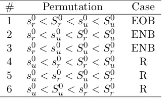
r < Sr0 and s0u < Su0, there are 6 possible permutations for these four numbers. If we have Sr0 > s0r > −∞, then all of the 6 permutations of s0r, Sr0, s0u and Su0 can be categorized into three cases, denoted by Case EOB, Case ENB and Case R, as shown in Table 3.1. Together with Case U, these four cases completely characterize the optimal ordering policy when the unreliable supplier is available.
Table 3.1: Possible permutations and their corresponding cases
# Permutation Case
1 s0
r < Sr0 < s0u < Su0 EOB 2 s0r < s0u < Sr0 < Su0 ENB 3 s0r < s0u < Su0 < Sr0 ENB 4 s0u < s0r < Sr0 < Su0 R 5 s0u < s0r < Su0 < Sr0 R 6 s0u < Su0 < s0r < Sr0 R
The ordering policy for each case can be explicitly stated as follows:
• When the unreliable supplier is down at the beginning of the period (J = 1), apply an
(s1r, Sr1) policy, where s1r and Sr1 are the reorder point and order-up-to point for the reliable supplier.
• When the unreliable supplier is up at the beginning of the period (J = 0),
1. When α ≥ b+ηcr−cr
b+ηcr−cu, Case U: order only from the unreliable supplier based on an
2. When α < b+ηcr−cr
b+ηcr−cu,
(i) Case EOB (s0
r < Sr0 < s0u): order from both suppliers or order from the unreliable supplier, based on the initial inventory levelx:
(qr, qu) = (Sr0−x, Su0−Sr0), forx≤s0r, (qr, qu) = (0, Su0−x), fors0r< x≤s0u, (qr, qu) = (0,0), forx > s0u.
(ii) Case ENB (s0r < s0u < Sr0): order from only one of the suppliers, based on the initial inventory levelx:
(qr, qu) = (Sr0−x,0), for x≤s0r, (qr, qu) = (0, Su0−x), for s0r < x≤s0u, (qr, qu) = (0,0), for x > s0u.
(iii) Case R (s0u < s0r): order only from the reliable supplier based on an (s0r, Sr0) policy.
From the optimal ordering policy, it is noted that orders are made exclusively from the unreliable supplier when it offers a reasonable price at a sufficiently high reliability level. On the contrary, orders are made from the reliable supplier only if the price difference between the two suppliers is not significant and the unreliable supplier is under high risk. For those circumstances in between, the retailer can either (i) order from both suppliers or order only from the unreliable supplier depending on the initial inventory level, which corresponds to Case EOB, or (ii) order from either the reliable supplier or the unreliable supplier depending on the inventory level, but not both, with respect to Case ENB.
literature has shown the optimality of a state dependent (s, S) policy for a supply system whose state is modeled by a Markov chain to reflect randomness in the supply process ( ¨Ozekici & Parlar, 1999; Song & Zipkin, 1996) and the optimality of an (s, S)-like policy for a system consisting of two perfectly reliable delivery modes with different lead times (Sethi et al., 2003). These results stimulate our interest in the domain where the (s, S)-like policy can be applied. Therefore, we consider two alternative models to better understand the scope of the optimality of an (s, S)-like policy. First, we consider a simpler model where the supply process is Bernoulli, a special case of the two-state Markov model in which the probability of disruption in the next period keeps the same whether the current period is disrupted or not. And it is assumed that the unreliable supplier is open to accept orders in each period but with a fixed nonzero probability the merchandise will not be delivered successfully. Other settings are similar to the previous finite horizon model. In this case, the state at the beginning of each period reduces to just the inventory level, and the t-period optimal cost can be written as
θt(x) = min
yu>yr yr>x
{Krδ(yr−x) +Kuδ(yu−yr) +cr(yr−x) +αcu(yu−yr) +αg(yu) + (1−α)g(yr)
+αηED[θt−1(yu−D)] + (1−α)ηED[θt−1(yr−D)]}.
(3.28) Similar analysis can be conducted and the resulting optimal policy for this model is the same (s, S)-like policy. Next, we investigate an alternative model when both suppliers are unreliable in terms of all-or-nothing delivery. Like the first model, we assume the supply process is Bernoulli. The only difference is that the two suppliers are both unreliable. Suppose that with probability α1 the order from supplier 1 will be successfully delivered, and with probability
α2 the order from supplier 2 will be successfully delivered, where α1 and α2 are independent.
the finite horizon model. The t-period optimal cost can be written as
θt(x) = min
y2>y1 y1>x
{K1δ(y1−x) +K2δ(y2−y1) +α1c1(y1−x) +α2c2(y2−y1) +α1α2g(y2)
+α1(1−α2)g(y1) + (1−α1)α2g(x+y2−y1) + (1−α1)(1−α2)g(x)
+α1α2ηED[θt−1(y2−D)] +α1(1−α2)ηED[θt−1(y1−D)]
+ (1−α1)α2ηED[θt−1(x+y2−y1−D)] + (1−α1)(1−α2)ηED[θt−1(x−D)]}.
(3.29) The numerical results (not shown) indicate that the ordering policy is not necessarily (s, S)-like. In summary, the (s, S)-like policy remains optimal for a supply system consisting of one reliable supplier and one unreliable supplier, no matter the uncertainty is modeled by Markov chain or Bernoulli distribution. However, such policy is no longer optimal when two unreliable suppliers are present.
3.4
Extension to an Infinite Horizon Model
It is pointed out by H. Scarf (1960) that even if the cost parameters and demand distribution are stationary, the optimal policy fails to be stationary due to the presence of a terminal cost incurred at the end of time horizon. This property naturally extends to our two supplier problem. In addition, the case category depends on the values of s0r, Sr0, s0u and Su0, which indicates that even the optimal case is not invariant across the time. Iglehart (1963) shows the convergence of the optimal (s, S) policy under a concave penalty cost. We find the similar convergence behavior in our finite horizon model. In this section, we provide a theoretical proof for the convergence of the optimal ordering policy. In addition, the limiting (s, S)-like policy characterizes the optimal ordering policy for the infinite horizon model.
satisfy the following Bellman equations:
θ0(x) = min
yu>yr yr>x
{Krδ(yr−x) +Kuδ(yu−yr) +cr(yr−x) +αcu(yu−yr) +αg(yu) + (1−α)g(yr)
+αηED[θ0(yu−Dt)] + (1−α)ηED[θ1(yr−D)]}, (3.30)
θ1(x) = min yr>x
{Krδ(yr−x) +cr(yr−x) +g(yr) +βηED[θ0(yr−D)] + (1−β)ηED[θ1(yr−D)]}. (3.31)
In order to obtain the convergence of the optimal ordering decision, we first need to investi-gate the limiting behavior of the cost function. The proof follows the spirit of Iglehart (1963). Assume the demand distribution and cost parameters are both stationary and let
V0(yr, yu, x, θ0t, θt1) =Krδ(yr−x) +Kuδ(yu−yr) +cr(yr−x) +αcu(yu−yr) +αg(yu) +(1−α)g(yr) +αηED[θ0t(yu−D)] + (1−α)ηED[θt1(yr−D)].
(3.32) Denote ˜yt,r0 (x),y˜t,u0 (x) (henceforth denoted byyt,r0 , yt,u0 for convenience) as the minimized values of yr, yu, respectively, given the initial inventory levelx, i.e.,
θ0t(x) = min
yu>yr yr>x
{V0(yr, yu, x, θ0t−1, θt1−1)}=V0(y0t,r, yt,u0 , x, θ0t−1, θt1−1). (3.33)
Since {y0
t,r, y0t,u},{yt0−1,r, yt0−1,u} are minimizing solutions to the t-period and (t −1)-period problems, respectively, we have
V0(y0t+1,r, yt0+1,u, x, θt0, θ1t)−V0(yt0+1,r, y0t+1,u, x, θ0t−1, θt1−1)≤θ0t+1(x)−θt0(x) ≤V0(y0t,r, y0t,u, x, θ0t, θt1)−V0(y0t,r, yt,u0 , x, θt0−1, θt1−1).
Therefore,
|θ0t+1(x)−θt0(x)| ≤max
V0(y0t+1,r, yt0+1,u, x, θt0, θ1t)−V0(yt0+1,r, y0t+1,u, x, θ0t−1, θt1−1) ,
V0(yt,r0 , y0t,u, x, θt0, θ1t)−V0(y0t,r, y0t,u, x, θt0−1, θt1−1) . (3.35)
Substituting the expression ofV0(·) into Eq. (3.35) yields
|θ0t+1(x)−θ0t(x)| ≤max
(1−α)η
Z ∞ 0
[θ1t(y0t+1,r−ξ)−θ1t−1(y0t+1,r−ξ)]f(ξ)dξ
+ αη Z ∞ 0
[θt0(y0t+1,u−ξ)−θt0−1(yt0+1,u−ξ)]f(ξ)dξ
,
(1−α)η
Z ∞ 0
[θ1t(y0t,r−ξ)−θ1t−1(yt,r0 −ξ)]f(ξ)dξ
+ αη Z ∞ 0
[θ0t(y0t,u−ξ)−θ0t−1(y0t,u−ξ)]f(ξ)dξ
. (3.36)
Due to the presence of holding cost, it is never optimal to order up to a very high inventory level, i.e., the sequences of order up to levels {S0
t,r},{S0t,u} are bounded above. Assume that ¯