©
DOI: 10.1534/genetics.104.031799
Coalescent-Based Association Mapping and Fine Mapping of Complex Trait Loci
Sebastian Zo
¨llner
1and Jonathan K. Pritchard
Department of Human Genetics, University of Chicago, Chicago, Illinois 60637 Manuscript received May 28, 2004
Accepted for publication October 21, 2004
ABSTRACT
We outline a general coalescent framework for using genotype data in linkage disequilibrium-based mapping studies. Our approach unifies two main goals of gene mapping that have generally been treated separately in the past: detecting association (i.e., significance testing) and estimating the location of the causative variation. To tackle the problem, we separate the inference into two stages. First, we use Markov chain Monte Carlo to sample from the posterior distribution of coalescent genealogies of all the sampled chromosomes without regard to phenotype. Then, averaging across genealogies, we estimate the likelihood of the phenotype data under various models for mutation and penetrance at an unobserved disease locus. The essential signal that these models look for is that in the presence of disease susceptibility variants in a region, there is nonrandom clustering of the chromosomes on the tree according to phenotype. The extent of nonrandom clustering is captured by the likelihood and can be used to construct significance tests or Bayesian posterior distributions for location. A novelty of our framework is that it can naturally accommodate quantitative data. We describe applications of the method to simulated data and to data from a Mendelian locus (CFTR, responsible for cystic fibrosis) and from a proposed complex trait locus (calpain-10, implicated in type 2 diabetes).
O
NE of the primary goals of modern genetics is to (1996) argued that, under certain assumptions, associa-understand the genetic basis of complex traits. tion mapping is far more powerful than family-based What are the genes and alleles that contribute to suscep- methods. They proposed that to unravel the basis of tibility to a particular disease, and how do they interact complex traits, the field needed to develop the technical with each other and with environmental and stochastic tools for genome-wide association studies (including a factors to produce phenotypes? genome-wide set of SNPs and affordable genotyping The traditional gene-mapping approach of positional technology). Those tools are now becoming available, cloning starts by using linkage analysis in families to and it will soon be possible to test the efficacy of genome-identify chromosomal regions that contain genes of in- wide association studies. Moreover, association mapping terest. These chromosomal regions are typically several is already extremely widely used in candidate gene stud-centimorgans in size and may contain hundreds of genes. ies (e.g.,Lohmuelleret al.2003).Next, linkage analysis is normally followed by linkage For all these studies, whether or not they start with disequilibrium and association analysis to help narrow linkage mapping, association analysis is used to try to de-the search down to de-the functional gene and active vari- tect or localize the active variants at a fine scale. At that ants (e.g.,Keremet al.1989;Hastbackaet al.1992). point, the data in the linkage disequilibrium (LD)-map-The positional cloning approach has been very success- ping phase typically consist of genotypes from asubset ful at identifying Mendelian genes, but mapping genes for of the common SNPs in a region. The investigator aims complex traits has turned out to be extremely challenging to use these data to detect unobserved variants that im-(Risch2000). Despite these difficulties, there have been pact the trait of interest. For complex traits, it will nor-a mounting number of recent successes in which posi- mally be the case that the active variants have a relatively tional cloning has led to the identification of at-risk modest impact on total disease risk. This small signal haplotypes or occasionally causal mutations, in humans will be further attenuated if the nearest markers are in and model organisms (e.g.,Horikawaet al.2000;Gre- only partial LD with the active site (Pritchard and
tarsdottiret al.2003; Korstan jeandPaigen2002; Przeworski2001). Moreover, if there are multiple risk
Laereet al.2003). alleles in the same gene, these will often arise on
differ-In view of the challenges of detecting genes of small ent haplotype backgrounds and may tend to cancel out effect using linkage methods,RischandMerikangas each other’s signals. [There is a range of views on how
serious this problem of allelic heterogeneity is likely to be for complex traits (Terwilliger andWeiss 1998;
1Corresponding author:Department of Human Genetics, University
Hugotet al.2001;Pritchard2001;ReichandLander
of Chicago, 920 E. 58th St., CLSC 507, Chicago, IL 60637.
E-mail: [email protected] 2001;Lohmueller et al.2003).]
Figure1.—Schematic example of the data structure. The lines indicate the chromosomes of three affected individuals (solid) and of three healthy control individuals (dashed). The solid circles indicate unobserved variants that increase disease risk. Each column of rect-angles indicates the position of a SNP in the data set. The goal is to use the SNP data to detect the presence of the disease variants and to estimate their location. Note that for a com-plex disease we expect to see the “at-risk” al-leles at appreciable frequency in controls, and we also expect to find cases without these al-leles. As a further complication, there may be multiple disease mutations, each on a different haplotype background.
For all these reasons, it is important to develop statisti- The current statistical methods in this field tend to be designed for one goal or the other, but in this article cal methods that can extract as much information from
the data as possible. Certainly, some complex trait loci we describe a full multipoint approach for treating both problems in a unified coalescent framework. Our aim can be detected using very simple analyses. However,
by developing more advanced statistical approaches it is to provide rigorous inference that is more accurate and more robust than existing approaches.
should be possible to retain power under a wider range
of scenarios:e.g., where the signal is rather weak, where In the first part of this article, we give a brief overview of existing methods for significance testing and fine the relevant variation is not in strong LD with any single
genotyped site (Carlsonet al.2003), or where there is mapping. Then we describe the general framework of our moderate allelic heterogeneity. approach. The middle part outlines our current imple-Furthermore, for fine mapping, it is vital to use a sensi- mentation, developed for case-control data. Finally, we de-ble model to generate the estimated location of disease scribe results of applications to real and simulated data. variants as naive approaches tend to underestimate the
uncertainty in the estimates (Morriset al.2002).
EXISTING METHODS In this article, we focus on the following problem.
Consider a sample of unrelated individuals, each
geno-Significance testing: The simplest approach to sig-typed at a set of markers across a chromosomal region
nificance testing is simply to test each marker separately of interest. We assume that the marker spacing is within
for association with the phenotype (using a chi-square the typical range of LD, but that it does not exhaustively
test of independence, for example). This approach is sample variation. In humans this might correspond to
most effective when there is a single common disease
⬇5-kb spacing on average (Kruglyak 1999;Zo¨ llner
variant and less so when there are multiple variants
and von Haeseler 2000; Gabriel et al. 2002). Each
(Slager et al. 2000). When there is a single variant,
individual has been measured for a phenotype of
inter-power is a simple function ofr2, the coefficient of LD
est, and our ultimate goal is to identify genetic variation
between the disease variant and the SNP (Pritchard
that contributes to this phenotype (Figure 1).
andPrzeworski2001) and the penetrance of the
dis-With such data, there are two distinct kinds of
statisti-ease variant. In some recent mapping studies, this sim-cal goals:
ple test has been quite successful (e.g.,Van Eerdewegh
et al.2002;Tokuhiroet al.2003). 1. Testing for association: Do the data provide evidence
The simplest multipoint approach to significance test-that there is genetic variationin this regionthat
con-ing is to use two or more adjacent SNPs to define haplo-tributes to the phenotype? (Typically, we would want
types and then test the haplotypes for association (Daly
to see a systematic difference between the genotypes
et al.2001;Johnsonet al.2001;Riouxet al.2001;
Gre-of individuals with high and low phenotype values,
tarsdottir et al. 2003). It is argued that
haplotype-respectively, or between cases and controls.) The
based testing may be more efficient than SNP-based strength of evidence is typically summarized using a
testing at screening for unobserved variants (Johnson
P-value.
2. Fine mapping: Assuming that thereisvariation in this et al.2001;Gabrielet al.2002). However, there is still uncertainty about how best to implement this type of region that impacts the phenotype, then what is the
most likely location of the variant(s) and what is the strategy in a systematic way and how the resulting power compares to other approaches after multiple-testing cor-smallest subregion that we are confident contains the
variant(s)? This type of information is conveniently rections.
posed for detecting disease association. These include Markov model for the LD between adjacent sites. The McPeek and Strahs model assumed a star-shaped geneal-a dgeneal-atgeneal-a-mining geneal-algorithm (Toivonenet al.2000),
multi-point schemes for identifying identical-by-descent re- ogy for the case chromosomes and applied a correction factor to account for the pairwise correlation of chromo-gions in inbred populations (Serviceet al.1999;Abney
et al.2002), and schemes for detecting multipoint associ- somes due to shared ancestry.
Subsequent variations on this theme have included ation in outbred populations (Lianget al.2001;Tzeng
et al.2003). other methods based on star-shaped genealogies (
Mor-ris et al.2000;Liu et al.2001) and methods involving Perhaps closest in spirit to the approach taken here
is the cladistic approach developed by Alan Templeton bifurcating genealogies of case chromosomes including those ofRannalaandReeve(2001),Morriset al.(2002), and colleagues (Templetonet al.1987; see also
Selt-manet al.2001). Their approach is first to construct a andLamet al.(2000). Two other methods have also used genealogical approaches, but seem to be practical only set of cladograms on the basis of the marker data by
using methods for phylogenetic reconstruction and for very small data sets or numbers of markers (Graham
andThompson1998;Larribeet al.2002).Morriset al.
then to test whether the cases and controls are
nonran-domly distributed among the clades. In contrast, the (2002) provide a helpful review of many of these methods. More recently,Molitoret al.(2003) presented a less inference scheme presented here is based on a formal
population genetic model with recombination. This model-based multipoint approach to fine mapping. They used ideas from spatial statistics, grouping haplotypes should enable a more accurate estimation of topology
and branch lengths. Our approach also differs from from cases and controls into distinct clusters and as-sessing evidence for the location of the disease mutation those methods in that we perform a more model-based
analysis of the resulting genealogy. from the distribution of cases across the clusters. Their approach may be more computationally feasible for
Fine mapping: In contrast to the available methods
for significance testing, the literature on fine mapping large data sets than are fully model-based genealogical methods, but it is unclear if some precision is lost by has a heavier emphasis on model-based methods that
consider the genealogical relationships among chromo- not using a coalescent model.
The procedure described in this article differs from somes. This probably reflects the view that a formal
model is necessary to estimate uncertainty accurately existing methods in several important aspects. Our ap-proach estimates the joint genealogy of all individuals,
(Morris et al. 2002), and that estimates of location
based on simple summary measures of LD do not pro- not just of cases. This should allow us to model the an-cestry of the sample more accurately and to include al-vide accurate assessments of uncertainty. The challenge
is to develop algorithms that are computationally practi- lelic heterogeneity in a more realistic way. We also ana-lyze the evidence for the presence of a disease mutation cal, yet extract as much of the signal from the data as
possible. The methods should work well for the interme- after inferring the ancestry of a locus. This enables us to apply realistic models of penetrance and to analyze diate penetrance values expected for complex traits and
should be able to deal with allelic heterogeneity. quantitative traits. Furthermore, in our Markov chain algorithm we do not record the full ancestral sequences Though one might ideally wish to perform inference
using the ancestral recombination graph (Nordborg at every node, which should enable better mixing and allow analysis of larger data sets.
2001), this turns out to be extremely challenging computa-tionally (e.g.,Fearnheadand Donnelly2001;Larribe
et al.2002). Instead, most of the existing methods make
MODELS AND METHODS progress by simplifying the full model in various ways
to make the problem more computationally tractable We consider the situation where the data consist of a sample of individuals who have been genotyped at a set (as we do here).
The first full multipoint, model-based method was of markers spaced across a region of interest (Figure 1). Each individual has been assessed for some phenotype, developed byMcPeek andStrahs (1999). Some
ele-ments of their model have been retained in most subse- which can be either binary (e.g., affected with a disease or unaffected) or quantitative. Our framework can also ac-quent models, including ours. Most importantly, they
simplified the underlying model by focusing attention commodate transmission disequilibrium test data ( Spiel-manet al.1993), where the untransmitted genotypes are only on the ancestry of the chromosomes at each of a
series of trial positions for the disease mutation. They treated as controls.
We are most interested in the setting where the geno-then calculated the likelihood of the data at each of
those positions and used the likelihoods to obtain a typed markers represent only a small fraction of the variation in the region, and our goal is to use LD and point estimate and confidence interval for the location
of the disease variant. Under that model, nonancestral association to detect unobserved susceptibility variants. We allow for the possibility of allelic heterogeneity (there sequence could recombine into the data set. The
these mutations occur close enough together (e.g., within a few kilobases) that we can treat them as having a single location within the region.
The genealogical approach: The underlying model for our approach is derived from the coalescent (re-viewed byHudson1990;Nordborg2001). The coales-cent refers to the conceptual idea of tracing the ancestry of a sample of chromosomes back in time. Even chromo-somes from “unrelated” individuals in a population share a common ancestor at some time in the past. Moving backward in time, eventually all the lineages that are ancestral to a modern day sample “coalesce” to a single common ancestor. The timescales for this process are typically rather long—for example, the most recent common ancestor of human-globin sequences is estimated to have beenⵑ800,000 years ago (Harding
et al.1997).
When there is recombination, the ancestral relation-ships among chromosomes are more complicated. At any single position along the sequence, there is still a single tree, but the trees at nearby positions may differ. It is possible to represent the full ancestral relationships
among chromosomes using a concept known as the “an- Figure2.—Hypothetical example of a coalescent genealogy cestral recombination graph” (ARG;Nordborg2001; for a sample of 28 chromosomes, at the locus of a disease
Nordborg andTavare 2002), although it is difficult susceptibility gene. Each tip at the bottom of the tree
repre-sents a sampled chromosome; the lines indicate the ancestral to visualize the ARG except in small samples or short
relationships among the chromosomes. The two solid circles chromosomal regions (Figure 3).
on the tree represent two independent mutation events pro-Considering the coalescent process provides useful ducing susceptibility variants. These are inherited by the chro-insight into the nature of the information about associa- mosomes marked with hatched circles. Individuals carrying tion that is contained in the data. Figure 2 shows a hypo- those chromosomes will be at increased risk of disease. This means that there will be a tendency for chromosomes from thetical example of the coalescent ancestry of a sample
affected individuals to cluster together on the tree, in two of chromosomes at the position of a disease
susceptibil-mutation-carrying clades. The degree of clustering depends ity locus. In this example, two disease susceptibility mu- in part on the penetrance of the mutation.
tations are present in the sample. By definition, these will be carried at a higher rate in affected individuals
than in controls. This implies that chromosomes from mation to learn as much as we can about the coalescent genealogy of the sample at different points along the affected individuals will tend to be nonrandomly
clus-tered on the tree. Each independent disease mutation chromosome. Our statistical inference for association mapping or fine mapping will be based on this. In what gives rise to one cluster of “affected” chromosomes.
Traditional methods of association mapping work by follows, we outline our approach of using marker data to estimate the unknown coalescent ancestry of a sample testing for association between the phenotype status and
alleles at linked marker loci (or with haplotypes). In and describe how this information can be used to per-form inference. Unlike in previous mapping methods effect, association at a marker indicates that in the
neigh-borhood of this marker, chromosomes from affected (e.g., Morris et al. 2002), we aim to reconstruct the genealogy of the entire sample and not just the geneal-individuals are more closely related to one another than
by random. Fundamentally, the marker data are infor- ogy of cases. This extension allows us to extract substan-tially more information from the data and enables sig-mative because they provide indirect information about
the ancestry of unobserved disease variants. Detecting nificance testing.
Performing inference:We start by developing some association at noncausative SNPs implies that case
chro-mosomes are nonrandomly clustered on the tree. notation. Consider a sample ofnhaplotypes fromn/2 unrelated individuals. The phenotype of individualiis In fact, unless we have the actual disease variants in
our marker set,the best information that we could possibly φi, and⌽represents the vector of phenotype data for
the full sample ofn/2 individuals. The phenotypes might
get about association is to know the full coalescent genealogy
of our sample at that position.If we knew this, the marker be qualitative (e.g., affected/unaffected) or quantitative measurements.
genotypes would provide no extra information; all the
infor-sibly from genome-wide scans). LetGdenote the multi- tion about the location of the disease mutation. Thus, we ignore the possible impact of selection and over-dimensional vector of haplotype data—i.e., the
geno-types forn haplotypes at L loci (possibly with missing ascertainment of affected individuals in changing the distribution of branch times at the disease locus. Our data). LetXbe the set of possible locations of the QTL
or disease susceptibility gene and letx僆 X represent expectation is that the data will be strong enough to overcome minor misspecification of the model in this its (unknown) position. Our approach is to scan
sequen-tially across the regions containing genotype data, con- respect (this was the experience ofMorriset al.2002, in a similar situation). The second approximation is a sidering many possible positions forx. A natural
mea-sure of support for the presence of a disease mutation good assumption if the active disease mutation is not actually in our marker set and if mutations at different at positionxis given by the likelihood ratio (LR),
positions occur independently. We can then write LR⫽ LA(⌽;x,Pˆalt,G)
L0(⌽;Pˆ0,G)
, (1)
Pr(⌽,G|x)⬇
冮
Pr(⌽|x,Tx)Pr(G|Tx)Pr(Tx)dTxwhereLAandL0represent likelihoods under the
alterna-and since Pr(G|Tx)Pr(Tx)⫽Pr(Tx|G)Pr(G) we obtain
tive model (disease mutation atx) and null hypothesis
(no disease mutation in the region), respectively. Pˆalt Pr(⌽,G|x)⬇
冮
Pr(⌽|x,Tx)Pr(Tx|G)Pr(G)dTx
andPˆ0are the vectors of penetrance parameters under
the alternative and null hypotheses, respectively, that ⬀
冮
Pr(⌽|x,Tx)Pr(Tx|G)dTx. (5)maximize the likelihoods. Large values of the likelihood ratio indicate that the null hypothesis should be
re-Expression (5) consists of two parts. Pr(⌽|x,Tx) is the
jected. Specific models to calculate these likelihoods
probability of the phenotype data given the tree atx. are described below (see Equations 7 and 8).
To compute this, we specify a disease model and then We also want to estimate the location of disease
muta-integrate over the possible branch locations of disease tions. For this purpose it is convenient to adopt a
Bayes-mutations in the tree (see below for details). Pr(Tx|G)
ian framework, as this makes it more straightforward
refers to the posterior density of trees given the marker to account for the various sources of uncertainty in a
data and a population genetic model to be specified; coherent way (Morriset al.2000, 2002;Liuet al.2001).
the next section outlines our approach to drawing The posterior probability that a disease mutation is at
Monte Carlo samples from this density.
xis then
In summary, our approach is to scan sequentially across the region(s) of interest, considering a dense set Pr(x|⌽,G)⫽ Pr(⌽,G|x)Pr(x)
兰XPr(⌽,G|y)Pr(y)dy
(2)
of possible positions of the disease locationx. At each positionx, we sampleMtrees [denotedT(m)
x ] from the
⬀Pr(⌽,G|x)Pr(x), (3)
posterior distribution of trees. For Bayesian inference of location, we apply Equation 2 to estimate the posterior where Pr(x) gives the prior probability that the disease
density Pr(x|⌽,G) atxby computing locus is atx. Pr(x) will normally be set uniform across
the genotyped regions, but this prior can easily be
modi-fied to take advantage of prior genomic information if Pr(x|⌽,G)⬇ (1/M)
兺
M
m⫽1Pr(⌽|x,T(xm))Pr(x)
兺
Yi⫽1(1/M)
兺
M
m⫽1Pr(⌽|yi,T(yim))Pr(yi)
, desired (see discussion in Rannala and Reeve 2001;
Morriset al.2002). (6)
To evaluate expressions (1) and (2), we need to
com-where {y1, . . . ,yY} denote a series of Ytrial values ofx
pute Pr(⌽,G|x). To do so, we introduce the notation
spaced across the region of interest. We will occasionally
Tx, to represent the (unknown) coalescent genealogy
refer to the numerator of Equation 6, divided by Pr(x), of the sample atx.Txrecords both the topology of the
as the “average posterior likelihood” at x. For signifi-ancestral relationships among the sampled
chromo-cance testing atx, we maximize somes and the times at each internal node. Then
Pr(⌽,G|x)⫽
冮
Pr(⌽,G|x,Tx)Pr(Tx|x)dTx LA(⌽;x,Pˆalt,G)⬇ 1M
兺
M
m⫽1
Pr(⌽|x,T(m)
x ,Pˆalt) (7)
⫽
冮
Pr(⌽|x,Tx)Pr(G|⌽,x,Tx)Pr(Tx|x)dTx, and(4) L0(⌽;Pˆ0,G)⫽Pr(⌽|Pˆ0) (8)
with respect toPˆaltandPˆ0. See below for details about
where the integral is evaluated over all possible trees. We
now make the following approximations: (i) Pr(Tx|x)⬇ how these probabilities are computed.
Sampling from the genealogy, Tx:To perform these
Pr(Tx) and (ii) Pr(G|⌽, x, Tx) ⬇ Pr(G|Tx). The first
approximation implies that in the absence of the pheno- calculations, it is necessary to sample from the posterior density,Tx|G (loosely speaking, we wish to draw from
informa-Figure 3.—Hypothetical example of the ancestral recombination graph (ARG) for a sample of six chromosomes, labeled A–F (left plot), along with our representation (middle and right plots). (Left plot) The ARG con-tains the full information about the ancestral relationships among a sample of chromo-somes. Moving up the tree from the bottom (backward in time), points where branches join indicate coalescent events, while splitting branches represent recombination events. At each split, a number indicates the position of the recombination event (for concrete-ness, we assume nine intermarker intervals, labeled 1–9). By convention, the genetic ma-terial to the left of the breakpoint is assigned to the left branch at a split. SeeNordborg (2001) for a more extensive description of the ARG. (Middle and right plots) At each point along the sequence, it is possible to ex-tract a single genealogy from the ARG. The plots show these genealogies at two “focal points,” located in intervals 4 and 7, respec-tively. The numbers in parentheses indicate the total region of sequence that is inherited without recombination, along with the focal point, by at least one descendant chromo-some. (1, 9) indicates inheritance of the en-tire region. For clarity, not all intervals with complete inheritance (1, 9) are shown.
the set of coalescent genealogies that are consistent with sample. It is likely that the region around the focal point shared by the three chromosomes is smaller. In our the genotype data). We adopt a fairly standard population
genetic model, namely the neutral coalescent with recom- representation of the genealogy, we store the topology at the focal point, along with the extent of sequence at bination (i.e., the ARG;Nordborg2001). Our current
implementation assumes constant population size. each node that is ancestral to at least one of the sampled chromosomes without recombination (Figure 3). A number of recent studies have aimed to perform
full-likelihood or Bayesian inference under the ARG An example of this is provided in Figure 4. Each tip of the tree records the full sequence (across the entire
(Griffiths andMarjoram 1996; Kuhneret al. 2000;
Nielsen 2000; FearnheadandDonnelly 2001;Lar- region) of one observed haplotype. Then, moving up
the tree, as the result of a recombination event a part
ribeet al.2002; reviewed byStephens2001). The
expe-rience of these earlier studies indicates that this is a of the sequence may split off and evolve on a different branch of the ARG. When this happens, the amount technically challenging problem, and that existing
methods tend to perform well only for quite small data of sequence that is coevolving with the focal point is reduced. The length of the sequence fragment that sets (e.g.,Wall2000;FearnheadandDonnelly2001).
Therefore, we have decided to perform inference under coevolves with the focal point can increase during a coalescent event, as the sequence in the resulting node a simpler, local approximation to the ARG, reasoning
that this might allow accurate inference for much larger is the union of the two coalescing sequences. In other words, the amount of sequence surrounding the focal data sets. Our implementation applies Markov chain
Monte Carlo (MCMC) techniques (seeappendix a). point shrinks when a recombination event occurs and may increase at a coalescent event. A marker is retained In our approximation, we aim to reconstruct the
coa-lescent tree only at a single “focal point” x, although up to a particular node as long as there is at least one lineage leading to this node in which that SNP is not we use the full genotype data from the entire region,
as all of this is potentially informative about the tree at separated from the focal point by recombination. We do not model coalescent events in the ARG where only that focal point. Consider two chromosomes that have
a very recent common ancestor (at the focal point). one of the two lines carries the focal point. Therefore, the sequence at internal nodes will always consist of one These chromosomes will normally both inherit a large
region of chromosome around the focal point, uninter- contiguous fragment of sequence.
Our MCMC implementation stores the tree topology, rupted by recombination, from that one common
Indeed, if one wished to perform inference across an infinitely long chromosomal region, the total amount of sequence stored at the ancestral nodes in our rep-resentation would be finite, while that in the earlier methods would not.
A more fundamental difference is that, unlike most of the previous model-based approaches to this prob-lem, our genealogical reconstruction is independent of the phenotype data. There are trade-offs in choosing to Figure4.—Example of an ancestral genealogy as modeled frame the problem in this way, as follows. When the by our tree-building algorithm. The ancestry of a single focal alternative model is true, the phenotype data contain point (designated F) as inferred from three biallelic markers
some information about the topology that could help is shown (alleles are shown as 0 and 1). Branches with
recombi-to guide the search through tree space. In contrast, our nation events on them are depicted as red lines, showing at
the tip of the arrow the part of the sequence that evolves on procedure weights the trees after sampling them from a different genealogy. As can be seen at the coalescent event Pr(Tx|G) according to how consistent they are with the at timet4, if no recombination occurs on either branch, the phenotype data (Equations 6 and 7), ignoring
addi-entire sequence is transmitted along a branch and coalesces,
tional information from the phenotype data. However, generating a full-length sequence. If on the other hand a
re-tackling the problem in this way makes it far easier to combination event occurs, the amount of sequence that reaches
the coalescent event is reduced (indicated by the dashes). If assess significance, because we know that under the null this reduction occurs on only one of the two branches, the the phenotypes are randomly distributed among tips of sequence can be restored from the information on the other the tree. It also means that we can calculate posterior branch (as at timet3). But if recombination events occur on
densities for multiple disease models using a single both branches, the length of the sequence is reduced (t2).
MCMC run.
Modeling the phenotypes:To compute expressions (6) and (7), we use the following model to evaluate Pr(⌽|x,Tx).
that are retained on each branch. (This rather simplistic
model is far more computationally convenient than At the unobserved disease locus, letAdenote the geno-type at the root of the treeTx. We assume that genotype
more realistic alternatives.) At some points, sequence is
introduced into the genealogy through recombination A mutates to genotype a at rate /2 per unit time, independently on each branch. We further assume that events. We approximate the probability for the
intro-duced sequence by assuming a simple Markov model on alleles in stateado not undergo further mutation. Next, we need to define a model for the genotype-the basis of genotype-the allele frequencies in genotype-the sample (similar
approximations have been used previously byMcPeek phenotype relationship for each of the three diploid genotypes at the susceptibility locus: namely, Pr(φ|AA),
andStrahs 1999; Morris et al. 2000; Liuet al. 2001;
Morriset al.2002). The population recombination rate Pr(φ|Aa), and Pr(φ|aa), whereφrefers to a particular phenotype value (e.g., affected/unaffected or a
quan- and the mutation rate are generally unknown in
advance and are estimated from the data within the titative measure). For a binary trait, these three proba-bilities denote simply the genotypic penetrances: e.g., MCMC scheme, assuming uniform rates along the
se-quence. A more precise specification of the model and Pr(Affected|AA). In practice, the situation is often com-plicated by the fact that the sampled individuals may not algorithms is provided inappendix a.
Overall, our model is similar to those of earlier ap- be randomly ascertained. In that case, the estimated “pene-trances” really correspond to Pr(φ|AA, S), Pr(φ|Aa, S), proaches such as the haplotype-sharing model ofMcPeek
andStrahs(1999) and the coalescent model ofMorris and Pr(φ|aa,S), whereSrefers to some sampling scheme
(e.g., choosing equal numbers of cases and controls).
et al.(2002). However, we focus on chromosomal
shar-ing backward in time, rather than on decay of sharshar-ing In the algorithm presented here, we assume that the affection status of the two chromosomes in an individual from an ancestral haplotype. In part, this reflects our
shift away from modeling only affected chromosomes can be treated independently from each other and from the frequency of the disease mutation:i.e.,PA(φ) isthe
to modeling the tree for all chromosomes. The
repre-sentation used by those earlier studies means that they probability that a chromosome with genotype A comes from an individual with phenotypeφ, and analogously forPa(φ). In
potentially have to sum over possible ancestral
geno-types at sites far away from the focal pointx, which are the binary situation, this model has two independent parameters:PA(1)⫽1⫺PA(0) andPa(1)⫽1⫺Pa(0).
not ancestral toany of the sampled chromosomes and
about which there is therefore no information. Storing In this case the ratioPA(φ)/Pa(φ) corresponds directly to
the relative risk of alleleA, conditional on the sampling all this extra information is likely to be detrimental in
an MCMC scheme, as it presumably impedes rearrange- scheme. As another example, for a normally distributed trait,PA(φ) and Pa(φ) are the densities of two normal
ments of the topology. Thus, we believe that our
repre-sentation can potentially improve both MCMC mixing distributions at φand would be characterized by mean and variance parameters. Note that most values ofPA(φ)
andPa(φ) do not correspond to a single genetic model Finally, it remains to determine the mutation rate,,
at the unobserved disease locus. It seems unlikely that that exists as the mapping from (PA(φ),Pa(φ)) to (Pr(φ|AA),
Pr(φ|Aa), Pr(φ|aa)) is dependent on the frequency of much information about will be in the data; hence we prefer to set it to a plausible value, a priori. For a the disease mutation. Nevertheless, this factorization of
the penetrance parameters is computationally conve- similar model,Pritchard(2001) argued that the most biologically plausible values for this parameter are in the nient and allows for an efficient analysis ofTx.
Of course, it is not known in advance which chromo- range ofⵑ0.1–1.0, corresponding to low and moderate levels of allelic heterogeneity, respectively.
somes areAand which area, so we compute the
likeli-hood of the phenotype data by summing over the possi- Multiple testing:Typically, association-mapping stud-ies consist of large numbers of statistical tests. To ac-ble arrangements of mutations at the disease locus.
Under the alternative hypothesis, most arrangements count for this, it is common practice to report aP-value that measures the significance of the largest departure of mutations will be relatively unsupported by the data,
while branches leading to clusters of affected chromo- from the null hypothesis anywhere in the data set. The simplest approach is to apply a Bonferroni correction somes will have high support for containing mutations.
LetMrecord which branches of the tree contain disease (i.e., multiplying the P-value by the number of tests), but this tends to be unnecessarily conservative because mutations and␥傺{1, . . . ,n} be the set of chromosomes
that carry a disease mutation according toM (i.e., the the association tests at neighboring positions are corre-lated.
descendants ofM) and letbe the set of chromosomes
that do not carry a mutation, i.e.,  ⫽ {1, . . . , n} \␥. A more appealing solution is to use randomization techniques to obtain an empirical overall P-value (cf. Then we calculate
McIntyre et al. 2000). The basic idea is to hold all
Pr(⌽|x,Tx,)⫽
兺
M冢
i兿
僆␥PA(φi)
兿
i僆Pa(φi)Pr(M|x,Tx,)
冣
. the genotype data constant and randomly permute thephenotype labels. For each permuted set, the tests of (9)
association are repeated, and the smallest P-value for that set is recorded. Then the experiment-wide signifi-For a case-control data set this can be written as
cance of an observedP-valuepiis estimated by the
frac-Pr(⌽|x,Tx,)⫽
兺
MPnA
d
A(1⫺PA)n
A
hPnad
a(1⫺Pa)n
a
hPr(M|x,T
x,), tion of random data sets whose smallest value isⱕp i.
The latter procedure is practical only if the test of where ni
d andnih count the number of i-type chromo- association is computationally fast. For the method
pro-somes (where i 僆 {A, a}) from affected and healthy posed in this article, the inference of ancestries is inde-individuals, respectively. Equation 9 can be evaluated pendent of phenotypes. Therefore, the trees need to efficiently using a peeling algorithm (Felsenstein1981). be generated only once in this scheme and the sampled The details of this algorithm are provided inappendix trees are stored in computer memory. Then, the
likeli-b. Calculations for general diploid penetrance models hood calculations can be performed on these trees using are much more computationally intensive, and we will both the real and randomized phenotype data to obtain present those elsewhere. the appropriate empirical distribution.
For our Bayesian analysis, we take the prior for the For a whole-genome scan, a permutation test with the parameters governing PA(φ) and Pa(φ) to be uniform proposed peeling strategy is rather daunting.
Per-and independent on a bounded set⌬˜ and average the forming the peeling analysis for 1000 permutations on likelihoods over this prior. By allowing any possible or- one tree of 100 cases and 100 controls takes ⵑ6 min der for the penetrances under the alternative model, on a modern desktop machine. Thus, a whole-genome we allow for the possibility that the ancestral allele may permutation test with one focal point every 50 kb, 100 actually be the high-risk allele, as observed at some hu- trees per focal point, and a penetrance grid of 19⫻19 man disease loci, including ApoE (Fullertonet al.2000). values would takeⵑ750,000 processor hours.
For significance testing, we test the null hypothesis that A rather different solution for genome-wide scans
PA(φ)⫽Pa(φ) compared to the alternative model where of association may be to apply the false discovery rate
the parameters governingPA(φ) andPa(φ) can take on criterion, as this tends to be robust to local correlation
any values independently. Standard theory suggests that when there are enough independent data (Benjamini
twice the log-likelihood ratio of the alternative model, andHochberg1995;Sabattiet al.2003).
compared to the null, should be asymptotically distrib- Unknown haplotype phase:Our current implementa-uted as 2 random values with d d.f., where d is the tion assumes that the individual genotype data can be
number of extra parameters in the alternative model resolved into haplotypes. However, in many current compared with the null. Thus, for case-control studies studies, haplotypes are not experimentally determined our formulation suggests that twice the log-likelihood and must instead be estimated by statistical methods. ratio should have a2
1distribution. In fact, simulations In principle, it would be natural to update the unknown
doing so, we would properly account for the impact of about the presence of disease variation will come from the degree to which case and control chromosomes haplotype uncertainty on the analysis. In fact,Morris
et al.(2004) concluded that doing so increased the accu- cluster on the tree, so bias in the branch length estimates may not have a serious impact on inferences about the racy of their fine-mapping algorithm (compared to the
answers obtained after estimating haplotypes via a rather location of disease variation. The next section provides results supporting this view.
simple EM procedure). However, it is already a difficult
problem to sample adequately from the posterior distri- Another factor not considered in our current imple-mentation is the possibility of variable recombination bution of trees givenknownhaplotypes and it is unclear
to us that the added burden of estimating haplotypes rate (e.g., Jeffreys et al. 2001). Since recombination rates appear to vary considerably over quite fine scales, within the MCMC scheme represents a sensible
trade-off. Therefore, we currently use point estimates of the this is probably an important biological feature to include in analysis. One route forward would be for us to estimate haplotypes obtained fromPHASE 2.0(Stephenset al.
2001;StephensandDonnelly2003). We also currently separate recombination parameters in each intermarker interval, within the MCMC scheme (perhaps correlated
usePHASEto impute missing genotypes.
False positives due to population structure: It has across neighboring intervals). It is unclear how much this would add to the computational burden of convergence long been known that case-control studies of association
are susceptible to high type 1 error rates when the sam- and mixing. In the short term, it would be possible to use a separate computational method to estimate these rates ples are drawn from structured or admixed populations
(LanderandSchork1994). Therefore, we advise using prior to analysis with local approximation to the
ances-tral recombination graph (LATAG;e.g., using Li and unlinked markers to detect problems of population
structure (PritchardandRosenberg 1999), prior to Stephens2003) and to modify the input file to reflect the estimated genetic distances.
using the association-mapping methods presented here.
When population structureisproblematic, there are Software:The algorithms presented here have been implemented in a program called LATAG. The program two types of methods that aim to correct for it: genomic
control (DevlinandRoeder1999) and structured asso- is available on request from S. Zo¨llner. ciation (Pritchardet al. 2000;Sattenet al. 2001). It
seems likely that some form of genomic control
correc-TESTING AND APPLICATIONS: SIMULATED DATA tion might apply to our new tests, but it is not clear to
us how to obtain this correction theoretically. It should To provide a systematic assessment of our algorithm we simulated 50 data sets, each representing a fine-be possible to obtain robust P-values using the
struc-tured association approach roughly as follows. First, one mapping study or a test for association within a candi-date region. Each data set consists of 30 diploid cases would apply a clustering method to the unlinked
mark-ers to estimate the ancestry of the sampled individuals and 30 diploid controls that have been genotyped for a set of markers across a region of 1 cM. Our model
(Pritchard et al. 2000; Satten et al. 2001) and the
phenotype frequencies across subpopulations. Then, the corresponds to a scenario of a complex disease locus with relatively large penetrance differences (since the phenotype labels could be randomly permuted across
individuals while preserving the overall phenotype fre- sample sizes are small) and with moderate allelic hetero-geneity at the disease locus.
quencies within subpopulations. As before, the test
sta-tistic of interest would be computed for each permuta- The data sets were generated as follows. We simulated the ARG, assuming a constant population size of 10,000 tion.
SNP ascertainment and heterogeneous recombination diploid individuals and a uniform recombination rate. On the branches of this ARG, mutations occurred as a
rates:In the MCMC algorithm described above, and more
fully inappendix a, we assume—for convenience—that Poisson process according to the infinite sites model. The mutation rate was set so that in typical realizations mutation at the markers can be described using a
stan-dard finite sites mutation model with mutation parame- there would be 45–65 markers with minor allele fre-quency⬎0.1 across the 1-cM region. The position of the ter. However, in practice, we aim to apply our method
to SNPs: markers for which the mutation rate per site disease locusxswas drawn from a uniform distribution
across the region. Mutation events at the disease locus is likely to be very low, but that have been specifically
ascertained as polymorphic. Hence, our estimate of were simulated on the tree at that location at rate 1 per unit branch length (in coalescent time), with no back should not be viewed as an estimate of the neutral
muta-tion rate; it is more likely to be roughly the inverse of mutations (cf. Pritchard 2001). This process deter-mines whether each chromosome does, or does not, the expected tree length (if there has usually been one
mutation per SNP in the history of the sample). More- carry a disease mutation. We required that the total frequency of mutation-bearing chromosomes be in the over, the fact that SNPs are often ascertained to have
intermediate frequency and that we overestimatemay range 0.1–0.2, and if it was not, then we simulated a new set of disease mutations at the same location. This lead to some distortion in the estimated branch lengths.
across the entire population, although many of the mu- posterior probability. The running time for each data set wasⵑ5 hr on a 2.4-GHz processor with 512 K memory. tations were redundant or at low frequency.
To assign phenotypes, we used the following pene- For comparison, we also analyzed each data set with DHSMAP-map 2.0 using the standard settings suggested trances: a homozygote wild type showed the disease
phenotype with probabilityPhw ⫽0.05, a heterozygous in the program package. This program generated point
estimates for the locus of disease mutation and two genotype showed it with probability Phe ⫽ 0.1, and a
homozygous mutant showed it with probability Phm ⫽ 95% confidence intervals: the first assuming a star-like
phylogeny among cases, and the second using a correc-0.8. According to these penetrances, we then created
30 case and 30 control individuals by sampling without tion to account for the additional correlation among cases that results from relatedness.
replacement from the simulated population of 20,000
chromosomes, as follows. Letnbe the remaining num- Significance tests were performed by two methods. First we calculated
ber of wild-type chromosomes in the population andm
be the remaining number of mutant chromosomes in
Lm⫽max {LA(⌽;xi,Palt,G) : i僆{1, . . . , 50},Palt僆⌬˜ }
the population. Then the next case individual was
ho-(10) mozygous for the mutation with probability (Phm·m ·
(m⫺ 1)) · (Phm·m· (m⫺1) ⫹2 · Phe·m·n ⫹Phw · and calculated the likelihood ratio according to (1), n · (n⫺ 1))⫺1, heterozygous with probability (2 ·P
he· m·n) · (Phm·m· (m⫺ 1)⫹2 ·Phe·m·n⫹Phw·n·
LR⫽ Lm
L0
, (n⫺1))⫺1, and otherwise homozygous for the mutant
allele. The diplotypes for each case were then created
by sampling the corresponding number of mutant or with L0⫽ 0.5120. We assigned pointwise significance to
wild-type chromosomes. Control individuals were gener- this ratio by assuming that 2 ln(LR) is 2-distributed
ated analogously. Across the 50 replicates, we found with 1 d.f. (Other simulations that we have done indicate that 10–33 of the 60 case chromosomes and 0–9 of the that this assumption is somewhat conservative; results control chromosomes carried a disease mutation. not shown.) To estimate global significance, we per-As might be expected for the simulation of a complex muted case and control status among the 60 individuals disease, not all of the simulated data sets carried much 1000 times, recalculatedLmfor each permutation (using information about the presence of genetic variation in- the original trees obtained from the data), and counted fluencing the phenotype. For instance, in 22 of the the number of permutations that showed a higherLm generated data sets, the highest single-point association than the original data set anywhere in the region. The signal among the generated markers, calculated as Pear- permutation procedure corrects for multiple testing son’s2, is⬍6.5.
across the region and does not rely on the predicted We analyzed each simulated data set by considering distribution of the likelihood ratio.
50 focal points x1, . . . , x50, spaced equally across the For comparison we assessed the performance of
sin-1-cM region. For each pointxiwe used LATAG to draw gle-point association analysis by calculating the
associa-50 trees from the distribution Pr(Txi|G,xi). To ensure tion of each observed marker in a 2 ⫻ 2-contingency
convergence of the MCMC, we used a burn-in period table with a2-statistic and recorded the2of the marker
of 2.5⫻106iterations forx
1. As the tree at locationxi with the highest value. We assigned significance to this
is a good starting guess for trees of the adjacent tree at test statistic in two ways: first, on the basis of the2 -distri-xi⫹1we used a burn-in of 0.5⫻106iterations forx2, . . . , bution with 1 d.f., and second, by performing 1000 xk. We sampled each set of trees {T(1)xi , . . . ,Tx(50)i } using permutations of phenotypes among the 60 individuals
a thinning interval of 10,000 steps and estimated Pr(⌽, and counting the number of permutations in which the
G|xi) according to (6) and (B2) without assuming any highest observed 2 was higher than that observed in
prior information about the location of disease muta- the sample.
tions. We found that the mean was somewhat unstable To assess convergence, we then repeated the analysis due to occasional large outliers and therefore substi- of each data set an additional four times and compared tuted the median for the average in (6). To evaluate (B2) the estimated posterior distributions to assess the con-we summed over a grid of penetrances⌬˜ ⫽ {0.05, 0.1, vergence of the MCMC and the variability in estimation. . . . , 0.95} ⫻ {0.05, 0.1, . . . , 0.95}, setting the disease We calculated the overlap of two credible intervalsC
1
mutation rateto 1.0. We calculated the posterior prob- andC
2obtained from multiple MCMC analyses of the
ability at each locusxiby evaluating same data set as
Pr(xi|⌽,G)⫽
Pr(⌽,G|xi)
兺
50j⫽1Pr(⌽,G|xj)
.
冢
|C1傽 C2||C1|
⫹|C1傽C2|
|C2|
冣
冒
2 ,
In addition, we recorded the point estimate for the
tively flat across the entire region. Some of the data sets contain very little information about the presence or location of disease mutations, and so small random fluc-tuations in the estimation can shift the peak from one part of the region to another. To further quantify this observation, we computed the correlation between the average pairwise difference of the point estimates with the average posterior likelihood at the point estimate for each data set. We observed that these were strongly negatively correlated (correlation coefficient⫽ ⫺0.29). The higher the signal that is present in the data (ex-pressed in posterior probability), the smaller the differ-ence is between the point estimates.
In summary, when the data sets contained a strong signal, the concordance between individual runs was Figure5.—Point estimates of the locus of disease mutation
quite high, indicating good convergence. On the other for five independent MCMC analyses of each of 50 simulated
data sets. The data sets are ordered from left to right by the hand, when the information about location was weak, median point estimate across the five replicates. The shading random variation across runs meant that the point esti-of the point indicates the strength esti-of the signal at the point
mates sometimes varied considerably. In such cases, estimate: darker points indicate stronger signals in the data.
longer runs would be needed to obtain really accurate Open points correspond to estimates where the average
poste-estimates. For analyzing real data, it is certainly impor-rior likelihood is⬍1.2-fold higher than the expected posterior
likelihood in the absence of disease mutations, shaded trian- tant to use multiple LATAG runs to ensure the ro-gles correspond to estimates that are 1.2–12-fold higher than bustness of the results.
the background, and solid circles correspond to estimates that
Point estimates of location:The mode of the posterior are⬎12-fold higher than background.
distribution is a natural “best guess” for the location of the disease variation. To assess the accuracy of this esti-mate, we calculated the distance between this point RESULTS
estimate and the real locus of the disease mutation for
Assessing convergence: An important issue for each simulated data set. Overall, we observed an average MC MC applications is to check the convergence of the error of 0.19 cM with a standard deviation of 0.23 cM. Markov chain, since poor convergence or poor mixing To evaluate this result, we compared it to the accuracy can lead to unreliable results. While numerous methods of two other point estimators. As a naive estimator, we exist to diagnose MC MC performance (Gammerman chose the position of the marker that has the highest
1997), the most direct approach is to compare the re- level of association with the phenotype, measured using sults from multiple MCMC runs. If the Markov chain the Pearson2statistic. This choice is based on the
ob-performs well, and the samples drawn from the posterior servation that, on average, LD declines with distance. are sufficiently large, then different runs will produce As an example of an estimator provided by a multipoint similar results. (Conversely, good performance by this method, we analyzed the prediction generated by criterion does not absolutely guarantee that the Markov DHSMAP.
chain is working well, but it is certainly encouraging.) We found that the average distance between the dis-To assess the convergence of the LATAG algorithm, ease locus and the SNP with the highest2was 0.25 cM
we performed five runs for each of the 50 simulated data (standard deviation 0.26 cM) and the distance to the sets. For our simulated data sets we found that on average, DHSMAP point estimate was 0.27 cM (standard devia-pairs of 50% credible intervals overlapped by 75% and tion 0.25 cM). The cumulative distributions of the error pairs of 95% credible intervals overlapped by 96%. in estimation are displayed in Figure 6. The estimate As a second method of evaluating the convergence generated by LATAG is most likely to be close to the of the MCMC, we compared the point estimates for the real locus of disease mutation. For instance, in 54% of location of disease mutation between the different runs. all simulations, the LATAG estimate is within 0.1 cM of The average distance between two point estimates on the the real locus, while the naive estimate is within 0.1 cM same data set is 184 kb. This number includes data sets in 44% of all cases and DHSMAP is in the same range where there is very little information about the locus of in 30% of our simulated data sets.
rela-Figure7.—Coverage accuracy of the credible intervals ob-tained by LATAG. We constructed credible intervals of differ-Figure6.—Cumulative distribution of distances (in
centi-ent sizes, ranging from 10 to 90% (x-axis). They-axis shows the morgans) between the locus of disease mutation and point
number of data sets (out of 50) for which the credible interval estimates from three different methods. From top to bottom,
contained the true location of the disease gene. The blue bars the three estimates are obtained from LATAG, DHSMAP, and
(number observed) are generally slightly higher than the pur-from the location of the SNP with the highest single-point
ple bars (number expected if the coverage is correct),
sug-2-value in a test for association.
gesting that our credible intervals may be slightly conservative.
of the posterior distribution for each data set. Figure 7
based 2 of 8.5. In 88% of the simulations, the2-test
plots the number of data sets for which the disease
mu-generated a more significant single-pointP-value. tation is located within each size credible interval and
However, because the extent of multiple testing may compares those numbers to the expected values. There
be different for the two methods, this is not exactly the is good accordance between the values, although it
ap-right comparison. The LATAG analysis consists of 50 pears that for low and intermediate confidence levels
tests, many of which are highly correlated, because the the constructed intervals are somewhat conservative and
trees may differ little from one focal point to the next. that the posterior distribution generated by LATAG
The SNP-based test consists of about the same number slightly overestimates the uncertainty. The high
uncer-of tests (one for each marker), and the correlation be-tainty about the location of the disease mutation is
re-tween tests depends on the LD bere-tween the markers. flected in the average size of the confidence intervals,
Therefore, a simple Bonferroni correction is too conser-which range from 0.06 cM for the 10% C.I. to 0.85 cM
vative for both test statistics. To perform tests that take for the 90% C.I.
the dependence structure in the data into account, we For comparison, we also looked at the 95% confidence
obtained P-values for each of the two test statistics by intervals that are generated by DHSMAP. Those intervals
permutation (seeSimulation methods). We observed that are considerably shorter than the intervals obtained from
correcting for multiple tests has a strong impact on the LATAG, at an average length of 0.37 cM for intervals
signal of the single-point analysis. For 24% of the data sets, obtained using the correction for pairwise correlation and
the single-point analysis produced a region-wideP-value 0.15 cM without that correction. But for both models the
⬍0.05, while in 30% of the data sets LATAG produced a confidence intervals were too narrow, with 48 and 18%,
P-value⬍0.05. Furthermore, the two tests do not always respectively, of intervals containing the true disease locus
detect the same data sets: one-third of all the data sets
(cf.Morriset al.2002). In summary, LATAG seems to
that showed a significant single-point score did not have provide credible regions that are fairly well calibrated or
a significant signal with LATAG, while 45% of all disease perhaps slightly conservative.
loci that were detected with LATAG were not detected
Hypothesis testing:To gauge the power of LATAG in
with the single-point analysis (Figure 8). Hence, although a test for association, we assessed for each data set whether
LATAG appears to be more powerful on average, there we could detect the simulated region as a region
harbor-may be some value in performing SNP-based tests of ing a disease mutation. To do this, we calculated the
association as well as that approach may detect some likelihood ratio at each focal point according to
Equa-loci that would not be detected by LATAG. tion 1 and considered the maximal LR that we observed
among all focal points as the evidence for association. For comparison, we also tested each SNP for association
TESTING AND APPLICATIONS: REAL DATA with the phenotype, using a standard Pearson 2-test.
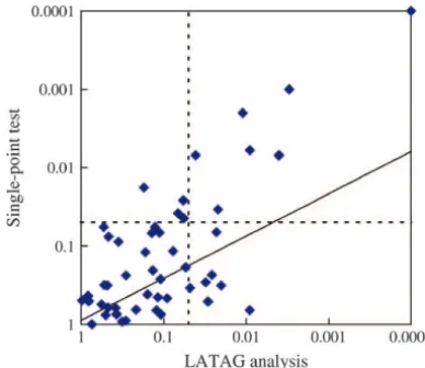
SNP-Figure 8.—Comparison of the ability of LATAG (x-axis) and a SNP-based2-test (y-axis) to detect disease-causing loci
Figure9.—Repeatability across runs. Average posterior like-in a test for association. Each polike-int corresponds to one of the
lihoods for 10 independent LATAG analyses of the CF data 50 simulated data sets and plots the most significantP-values
set are shown. For the location of the disease locus and the obtained for that data set using each method, corrected for
resulting posterior credible region refer to Figure 10. multiple testing within the region. The dotted lines depict
theP⫽0.05 cutoffs and the diagonal line plots the regression line through the log-log-transformed data.
calculated P(⌽|Ti, x) with the peeling algorithm. As
the resulting posterior likelihoods seemed to be heavily dependent on a few outliers, we estimated the likelihood map the gene responsible for cystic fibrosis, a simple
recessive disorder (Keremet al.1989), while the other P(x|⌽,G) at each position xby taking the median of the likelihoods P(⌽|Ti, x) instead of the average
sug-data set is from a positional cloning study of a complex
disease, type 2 diabetes (Horikawaet al.2000). gested by theory. As before, we used the posterior mode as our point estimate for location. Missing data were
Example application 1:Cystic fibrosis:The cystic
fibro-sis (CF) data set used byKeremet al.(1989) to map the imputed using PHASE 2.0 (Stephenset al.2001).
Results: To provide a simple check of convergence, CFTR locus has been used to evaluate several previous
fine-mapping procedures, thus allowing an easy compar- Figure 9 shows the results from the 10 independent analy-ses of the CF data set. As can be seen, all 10 runs have ison between LATAG and other multipoint methods.
The data set was generated to find the gene responsible modes in the same region and yield the same conclusion about the location of the causative variation.
for CF, a fully penetrant recessive disorder with an
inci-dence of 1/2500 in Caucasians. Many different disease- Figure 10 summarizes our results across the 10 runs. The posterior distribution is sharply peaked at 867 kb, causing mutations have been observed at the CFTR
lo-cus, but the most common mutation,⌬F508, is at quite near the true location of⌬F508 (which is at 885 kb). The 95% credible interval is rather narrow, extending high frequency, accounting for 66% of all mutant
chro-mosomes. from 814 to 920 kb. Even though several markers with little association to the trait are in the vicinity of the The data set consists of 23 RFLPs distributed over
1.8 Mb; these were genotyped in 47 affected individuals. deletion (Figure 10), the LATAG estimate is quite accu-rate. It is useful to compare our results to those obtained In addition, 92 control haplotypes were obtained by
sampling the nontransmitted parental chromosomes. by other multipoint methods (see Table 1, modified
fromMorriset al.2002). For this data set, most of the
High levels of association were observed for almost all
markers in the region; the marker with the highest highest single-point2values lie to the left of the true
location of⌬F508, and so most of the methods err to single-point association (2 ⫽ 63) is located at 870 kb
from the left-hand end of the region. The⌬F508 muta- the left, with some of the earliest methods (
Terwil-liger1995) actually excluding the true location from
tion is at 885 kb and is present in 62 of the 94 case
chromosomes. the confidence interval. Note that the LATAG estimate is closer to the true location, and that the 95% credibility We ran 10 independent runs of the Markov chain,
estimating the average posterior likelihood at each of region is narrower than that obtained by any of the previous methods.
50 evenly distributed points across the region. Each run
had a burn-in of 2.5⫻106steps for the first focal point To assess the ability of LATAG to detect the CF region
by association, we calculated a likelihood ratio accord-and 106 steps for each following focal point. In each
run, we sampled 50 trees at each focal point, with a ing to (1) and obtained 2 ln(LR) ⫽ 40. Assuming a
2-distribution with 1 d.f., this log-likelihood ratio has an
thinning interval of 10,000 steps. The runs took 8 hr