Mapping Quantitative Trait Loci From a Single-Tail Sample of the Phenotype Distribution Including Survival Data

DOI: 10.1534/genetics.107.081299

Mapping Quantitative Trait Loci From a Single-Tail Sample of

the Phenotype Distribution Including Survival Data

Mikko J. Sillanpa¨a¨*

,1

_{and Fabian Hoti*}

,†

*Department of Mathematics and Statistics, University of Helsinki, FIN-00014 Helsinki, Finland and †_{National Public Health Institute, Department of Vaccines, FIN-00300 Helsinki, Finland}

Manuscript received August 29, 2007 Accepted for publication October 5, 2007

ABSTRACT

A new effective Bayesian quantitative trait locus (QTL) mapping approach for the analysis of single-tail selected samples of the phenotype distribution is presented. The approach extends the affected-only tests to single-tail sampling with quantitative traits such as the log-normal survival time or censored/selected traits. A great benefit of the approach is that it enables the utilization of multiple-QTL models, is easy to incorporate into different data designs (experimental and outbred populations), and can potentially be extended to epistatic models. In inbred lines, the method exploits the fact that the parental mating type and the linkage phases (haplotypes) are known by definition. In outbred populations, two-generation data are needed, for example, selected offspring and one of the parents (the sires) in breeding material. The idea is to statistically (computationally) generate a fully complementary, maximally dissimilar, observation for each offspring in the sample. Bayesian data augmentation is then used to sample the space of possible trait values for the pseudoobservations. The benefits of the approach are illustrated using simulated data sets and a real data set on the survival of F2 mice following infection with Listeria monocytogenes.

Q

UANTITATIVE trait locus (QTL) mapping meth-ods often assume that the trait, conditionally on the effects of the QTL, follows a normal distribution. However, nonrandom missing data patterns resulting from single-tail sampling may violate this assumption. The target in single-tail sampling is to increase the ex-pected genotype–phenotype correlation of a sample with respect to the original population parameters. By sam-pling (ascertaining) individuals from the right tail of the phenotype distribution, the genotype frequencies for QTL with positive phenotype effects are potentially en-riched. Similarly, sampling individuals from the left tail of the phenotype distribution can increase our chances to find QTL with negative effects. Single-tail sampling may also arise from censoring or if a quantitative trait exhibits measurable values only for a portion of the in-dividuals,i.e., there is a spike in the phenotype distribution (Broman2003). However, due to single-tail sampling, the phenotypic variation of a sample may become too small for standard QTL mapping methods to work properly,i.e., the signal is totally masked by the error. Therefore current approaches to QTL mapping of data resulting from single-tail sampling of the phenotype distribution consider the deviation of the allele- (or genotype-) frequency distri-bution at the marker loci from their Mendelian expec-tation, use logistic regression-based analysis strategies,

or combine both of these approaches (Henshalland Goddard1999; Beasleyet al.2004; Tenesaet al.2005). Alternatively one can apply nonparametric/semipara-metric methods, rank-based statistical procedures, or a robust mixture model to analyze such data (Kruglyak and Lander1995; Zouet al.2002, 2003; Broman2003; Feenstraand Skovgaard2004). A disadvantage of these approaches is that a single-QTL model is implicitly as-sumed, since only a single chromosomal position is tested at a time.

As stated in Luoet al.(2005), the viability (survival) of an individual can be simply defined as a binary phe-notype indicating whether an individual has survived (y ¼ 1) or not (y ¼ 0). For continuous survival (or failure) time data, such as time to tumor or time to death (measured in logarithmic scale), the single-tail sampling approach can be considered (Broman2003). Alternatively, methods exist for survival phenotypes (Diao et al. 2004; Moreno et al. 2005). In controlled crosses, several methods have been designed specially to map viability loci, the gene positions that have an influence on the fitness or the survival of an individual (e.g., Vogland Xu2000; Luoand Xu2003; Luoet al. 2005; Nixon 2006). In outbred populations, similar/ related methods are adopted to locate the signatures of selection—the genomic regions having been under selective pressure (subject to natural or artificial selec-tion). It is well known that (1) the variability (diversity) is reduced, (2) the linkage disequilibrium is enriched, and (3) the segregation ratios depart from their 1_{Corresponding author:Department of Mathematics and Statistics, P.O.}

Box 68, University of Helsinki, FIN-00014 Helsinki, Finland. E-mail: [email protected]

Mendelian expectations in the genomic regions at the immediate surroundings of the gene positions that influence survival. The size of the effect (selection in-tensity) the position has on the survival can be indirectly monitored via the extent of the above influences and their decay as a function of the genetic distance. Thus, the general rationale behind the mapping methods of such loci is in testing distorted segregation, testing linkage disequilibrium patterns, or comparing levels of genetic variability between the particular genomic posi-tion and other parts of the genome or between species. Again, as a drawback, a single-QTL model is usually implicitly assumed in these methods. Moreover, a com-mon difficulty in applying these methods in outbred populations is that the demographic history (popula-tion growth or recent expansion) leaves kinds of local signs in the genome similar to those of selection (e.g., Schlo¨ tterer2003).

For case–control and association studies of binary traits in human genetics, it is common that one samples affected individuals only (see Greenland1999). There is the affecteds-only test for trios, where genotyped or haplotyped parents and their affected offspring are both collected (e.g., Falk and Rubinstein 1987; Terwilligerand Ott1992; Landerand Schork1994; Gauderman et al. 1999). Such a test is constructed between the cases and the controls where the individ-uals of the control sample, so-called pseudocontrols, ‘‘artificial controls,’’ or ‘‘antisibs,’’ are created from the genetic material that was not transmitted from the parents to the cases (their chromosomes are mirror images of the case chromosomes). The information needed to generate the chromosomes for the antisibs is obtained from the parental haplotypes by taking the complement of the genetic material of the parents that was transmitted to the affected offspring (see Figure 1). The ability to derive such a complement on the basis of the parental genotype data depends only on the parental mating type for the marker (marker informa-tiveness);e.g., it is easy to derive complemental obser-vations for mating typeAB3CD. Some single-locus tests

also utilize genotypic pseudoobservations in 1:3 propor-tions. By adopting the pseudocontrol approach, one can obtain well-matched controls and avoid spurious associations due to ethnic confounding,i.e., closer kin-ship (higher degree of background linkage disequilib-rium) in the affected sample (Terwilligerand Weiss 1998).

Here we bring this antisib idea to mapping QTL in experimental crosses (e.g., backcross and F2) of inbred lines as well as provide a theoretical basis for applying this method to outbred populations using a multiple-QTL model. To illustrate the methodology, we extend the affected-only tests to single-tail sampling with quan-titative traits. In the method, continuous-trait values are generated for all of the antisibs on the basis of Bayesian hierarchical modeling and data augmentation. For data augmentation, see Albert and Chib (1993), Rubin (1996), and Van Dykand Meng(2001). Unlike many others who consider mapping QTL (for quantitative, viability, or survival data) from single-tail samples, we use a multiple-QTL model.

To map signatures of selection, viability, and other binary traits from case-only data (where only selected/ survived individuals are in our sample and have pheno-typic value one), it is straightforward to genotype individ-uals from the single-phenotypic group only (i.e., survived individuals). In the continuous-trait case, one can selec-tively sample backcross or F2progenies so that the (case) individuals from only one tail of the phenotype distri-bution are genotyped. Pseudocontrols, corresponding to observations from the other tail of the phenotype distribution, can then be created as mirror images for each case individual. The binary phenotypic value of the pseudocontrol individuals is zero and their continuous-scale observations (so-called liability values) can be pre-dicted using data augmentation. (Note that the liability values of the case individuals are already observed.) The genotype data for these artificial observations can be created on the basis of the genotypes and linkage phases of the parents, which in inbred line-cross designs are known by definition. For example, in backcross, one can

Figure1.—A general representation on how

follow the principle that the mirror image of genotype AAisABand vice versa. In F2, the mirror images of the three genotypesAA,AB,BBareBB,AB,AA, respectively. The same principle applies for outbred crosses and populations where the parental genotypes and haplo-types are known or estimated.

MODEL

Notation:Let us consider an inbred line-cross experi-ment (e.g., backcross, double haploids, or F2) withNgen possible genotypes. We assume that measurements of a quantitative trait and marker genotypes atN loci have been obtained from Nind individuals sampled from a single tail of the phenotype distribution. To consider a pseudocontrol idea (Figure 1) for quantitative traits, it is easy to adopt a liability and threshold model framework (e.g., Albertand Chib1993). Further, we assume that each sample has a mirror image (hidden observation) in the unsampled part of the phenotype distribution. Using case–control and threshold model terminology this assumption means that for each case individual (whose liability value is measured) we need one control individual (whose liability value is systematically lower/ greater than that in case individuals).

Denote the phenotype and marker data of the ob-served offspring as (yo_,Mo_{) and the hidden phenotype}

and marker measurements of the offspring data as (yh_,Mh_{). From here on we refer to individualiand its}

unobserved counterpart as pair i. (Note that survival data, where genotypesMh_{are observed for censored}

in-dividuals, are a special case of this setting.) The observed and hidden phenotype vectors,yo_{¼ ðy}o

1;. . .;y o

NindÞ and yh_{¼ ðy}h

1;. . .;y h

NindÞ; include the observed and hidden phenotypes of pair i,yo

i and y

h

i;respectively. Similarly, Mo_{¼ ðm}o

i;jÞ and M

h_{¼ ðm}h

i;jÞ are the observed and

hidden marker matrices where the elements, mo

i;j and mh

i;j, are the coded genotypes from the set½1,. . .,Ngen for pairion markerj. To allow that some marker geno-types may be missing among the observed half of the individuals, the incomplete form ofMo _{is denoted by}

M*¼ ðmi*;jÞ: Note that if there are no missing marker

genotypes, thenMo_¼M*.

To exploit the ‘‘mirroring idea’’ by applying data augmentation on the hidden observations (yh_,Mh_{), it is}

helpful to consider that the observed phenotypes (yo₎

give rise to the discrete auxiliary variables (discrete phenotypes). Let zo_{¼ ðz}o

1;. . .;z o

NindÞ denote a discrete phenotype vector where for individuali, zo

i ¼1fyo

i.Tg:

Here T is a (known) discretization threshold and the binary phenotypezo

i obtains value 1 if the underlying

(observed) continuous phenotypeyo

i is higher than the

threshold T and zo

i ¼ 0 otherwise. Similarly, for the

hidden observationsyh_{, we have a discrete vectorz}h_¼

zh 1;. . .;z

h

Nind

;wherezh

i ¼1fyh

i .Tg¼1z

o

i:To conclude,

in single-tail sampling, (1) the threshold T uniquely determines the proportion of individuals selected from

the phenotype distribution, (2) all elements in vectorzo

are either 0 or 1, and (3) all elements in vector zh_are

either 0 or 1 and opposite tozo_{. In the case thatTis}

un-known, depending on which tail has been sampled we can defineT as the smallest or the highest phenotype value. Phenotype model: We adopt the additive multiple-QTL model considered earlier by Xu(2003). This model is closely related to the model of Meuwissenet al.(2001) and can be viewed as a submodel of Hoti and Sillanpa¨ a¨ (2006). Although it is straightforward to include also pairwise epistatic interaction terms in the design matrix of this model (see Zhangand Xu2005; Xu2007), we omit such extensions here. For considering other models and designs, see thediscussion. In the model, let us assume that the putative QTL can be placed only at marker points. However, this is not a very restrictive assumption because in experimental designs, arbitrary map positions (putative QTL) can be included into the analysis as pseudomarkers (Senand Churchill2001). Given the overall meana and the effect-specific coefficientsb¼(bj,k) of markerj,

the phenotypesys

i;s¼o,hof the pairican be expressed as

ys_i ¼a1 X

N

j¼1 X

Ngen

k¼1

b_j;k1fms i;j¼kg1e

s

i; ð1Þ

where the residuals (the phenotypes after correcting for QTL effects) are assumed to be normally distributed, es

i Nð0;s

2

eÞ;with unknown variances

2

e:Note that this

same model is assumed for both the observedðyo

iÞand

the hidden ðyh

iÞ phenotypes. The indicator variable

1fms

i;j¼kg¼1 if the marker observationm s

i;j equals

geno-type code kand is 0 otherwise. For each markerj we introduce the constraintbj,1¼0. Thus for a backcross or double haploids, where Ngen ¼ 2, only a single co-efficient bj,2at each marker is needed to capture the contrast between the two genotypes. Similar treatment for F2, whereNgen¼3, leads to two coefficients,bj,2and bj,3, that can be estimated for each marker. Here we use a random-variance model, where the genetic coeffi-cients b_j,k, fork. 1, are assumed to be normally dis-tributed Nð0;s2

j;kÞwith unknown variancess

2

j;k:In the

following, we denote all unknown QTL parameters together asu¼ ða;b;s2;s2

eÞ;wheres

2_{¼ ðs}2

j;kÞis a

vec-tor of the effect-specific variances.

Key assumptions (which should be considered jointly because assumption 1 is a necessary condition for as-sumption 2):

approaches that try to maximize the information in the sample by selecting individuals or pairs of indi-viduals to be phenotyped on the basis of their genetic dissimilarity (Jinet al.2004; Jannink2005; Xuet al. 2005; Fuand Jansen2006).

2. The phenotypes of the hidden observations are (gen-erated using data augmentation) either on the left or the right side of the truncation point and the observed phenotypes: We briefly consider what is assumed at the genetic level, in the presence of the additive multiple-QTL model (1), when ‘‘mirroring’’ of the genotypes is performed. Now, we assume ordering of the phenotypes with respect to the thresholdT:

y_ih#T#yo_i for all pairsi: ð2Þ

To see what this means at the genetic level, we substitute model (1) into both sides of Equation 2 so thatacancels out, and we obtain

XN

j¼1 X

Ngen

k¼1

b_j;k1fmh

i;j¼kg1e

h

i #T#

XN

j¼1 XNgen

k¼1

b_j;k1fmo

i;j¼kg1e

o

i;

ð3Þ

where residuals eh

i and e

o

i are both independently

normally distributed with mean zero. Let us consider the following cases:

i. When the residuals are orderedeh

i #e

o

i in the same

way as phenotypes of Equation 2: For such pairs i, Equation 3 imposes an ordering constraint for the sum of the QTL effects that the mirrored genotypes at the QTL loci need to fulfill. However, this ordering constraint is relaxed by the nonnegative factorfi ¼ eo

i e

h

i: This means that the model can cope with

some proportion of phenocopies (i.e., such data indi-viduals whose phenotype is not in agreement with the QTL model).

ii. When the residuals are orderedeh

i .e

o

i in the opposite

way as the phenotypes of Equation 2: For such pairsi, the ordering constraint is adjusted by the negative factorfi ¼eioe

h

i:This means that for some of the

phe-notypes it is required that the ordering constraint is ful-filled in a tighter form. We now represent Equation 3 as

XN

j¼1 XNgen

k¼1

b_j;k1fmh

i;j¼kg#

XN

j¼1 XNgen

k¼1

b_j;k1fmo

i;j¼kg1fi; ð4Þ

wherefi ¼eioe

h

i is a relaxation/adjustment factor

of the ordering constraint, whose sign and size de-pend on the rank and the difference of the two re-siduals, respectively. Further understanding of this question requires simulation studies that are not in the scope of this article.

Assumptions 1 and 2 together imply that each sample has a mirror image (hidden observation) in the un-sampled part of the phenotype distribution.

Hierarchical model:In Bayesian analysis, the aim is to obtain an estimate for the posterior distribution of the model parameters given the data,p(u,yh_,Mh_,Mo_,zo_,zh_j

yo_{, M*). This can be achieved by using Markov chain}

Monte Carlo (MCMC) methods, exploiting the fact that the posterior is proportional to the joint distribution of the parameters and the data,p(u,yh_{, M}h_,Mo_,zo_,zh_,yo_,

M*). By adopting suitable conditional independence assumptions (leading to the graphical model of Figure 2), the joint distribution of the parameters and the data can be presented as

pðu;yh;Mh;Mo;zo;zh;yo;M*Þ

¼pðzhjzo;yhÞpðzojyoÞpðyo;yhju;Mo;MhÞ 3pðMhjMoÞpðM*jMoÞpðMoÞpðuÞ;

where the likelihood can be factorized as

pðyo;yhju;Mo;MhÞ

¼pðyoju;MoÞpðyhju;MhÞ

¼Y

Nind

i¼1 YN

j¼1

pðy_ioju;M_io;jÞ

Y

Nind

i¼1 YN

j¼1

pðyh_i ju;M_ih;jÞ:

The functional forms ofp(yo

i ju,M

o

i;j) andp(y

h

i ju;M

h

i;j)

are normal densities of the residualseo

i ande

h

i of model

(1) with mean zero and variances2

e (see,e.g., Sillanpa¨ a¨

and Arjas1998).

Constraining priors: This model includes an excep-tionally high number of constraining priors, which introduce restrictions into the (MCMC) sampling scheme and take care of the consistency between vari-ables. Their specific forms are given below. The prior for the discretized hidden observations is pðzh_jzo_;yh_{Þ ¼}

QNind

i¼1pðz h

i jz

o

i;y

h

iÞ;where p(z

h

i jz

o

i;y

h

iÞ ¼pðz

h

i jz

o

iÞpðz

h

i jy

h

i).

Here, pðzh

i ¼1jz

o

iÞ ¼1fzo

i¼0g;pðz

h

i ¼0jz

o

iÞ ¼1fzo

i¼1g; pðzh

i ¼1jy

h

iÞ ¼1fyh

i.Tg; and pðz

h

i ¼0jy

h

iÞ ¼1fyh

i#Tg:

Moreover, the prior for the discretized ‘‘nonhidden’’ observations ispðzo_jyo_{Þ ¼}QNind

i¼1pðz o

i jy

o

iÞ;wherepðz

o

i ¼

1jyo

iÞ ¼1fyo

i.Tg andpðz

o

i ¼0jy

o

iÞ ¼1fyo

i#Tg:The

mark-ers of the pseudoobservations are created according to the mirroring priorpðMh_jMo_{Þ ¼}QNind

i¼1

QN

j¼1pðmih;jjm

o

i;jÞ;

wherepðmh

i;j¼1jmio;jÞ ¼1fmo

i;j¼0gandpðm

h

i;j¼0jmoi;jÞ ¼

1fmo

i;j¼1g:Also the indicator function priorpðM*jM

o_{Þ ¼}

1fMo_{is consistent withM*g}is used to ensure that the complete marker observations are compatible with the observed data.

Other priors:In inbred line-cross data, the prior used to handle missing observations can be presented as a Markov chain pðMo_{Þ ¼}QNind

i¼1

pðMo

i;lÞ QN

j¼2pðM o

i;jjM

o

i;j1Þ

: For the actual forms of the transition probabilities pðMo

i;jjM

o

i;j1) in various designs, see Jiangand Zeng (1997) and Sillanpa¨ a¨and Arjas(1998). The prior for the QTL parameters can be factorized as p(u)¼p(a) p(bjs2_)p(s2_)p(s2

e), where p(a) } 1, pðbjs

2_{Þ ¼}QN j¼1

QNgen

k¼2pðbj;kjs2j;kÞ, and pðs

2_{Þ ¼}QN j¼1

QNgen

k¼2pðs2j;kÞ:

distribution with mean zero and variance s2

j;k; and pðs2

j;kÞ}1=s

2

j;kis the Jeffreys scale invariant prior having

most of the support (mass) in values near zero. Also, for the residual variance, we choosepðs2

eÞ}1=s2e:The use

of effect-specific variance components together with Jeffreys’ prior is well justified because the prior adap-tively shrinks QTL variances at unlinked positions to zero—which then leads to the positioning of QTL with nonnegligible effects (see Xu2003; Hotiand Sillanpa¨ a¨ 2006). Note that Meuwissenet al.(2001) fitted a com-mon variance for all coefficients at single locus, which, however, does not lead to an equally sparse solution. It is good to know that even if Jeffreys’ prior in this context seems to work extremely nicely, theoretically the poste-rior is improper because Jeffreys’ pposte-rior has an infinite amount of mass near zero (e.g., Hopertand Casella 1996; ter Braak et al. 2005). One way to avoid the theoretical problem is to specify a small positive number as a lower bound for the parameter in the prior, which we, however, did not apply here.

Parameter estimation: We use a MCMC algorithm

(e.g., Casellaand George1992; Chiband Greenberg 1995) to estimate the posterior distribution of the un-known model parameters. Here we assume that the truncation pointTof the original population is known, equals the smallest (or the highest) phenotypic value in the data, or has been successfully estimated before the analysis. Also if the phenotypic meanyof the original population is available, we can utilize it as a starting value fora; otherwise we initializeato zero (i.e., we set

y¼0). We use nonzero starting values for the variances so that nonzero values are proposed for all effects—all

positions initially explain the phenotype. In the follow-ing, we outline the MCMC sampling scheme used for continuous traits. For survival data, if genotypesMh_are

observed/available for censored individuals, we can omit the generation of mirror images in steps 1 and 3. For binary traits, step 4 below is replaced by the step ‘‘the updating liabilities for a binary trait’’ found in earlier articles (Kilpikari and Sillanpa¨ a¨ 2003; Hoti and Sillanpa¨ a¨2006):

1. Specify initial valuesa¼y, (bj,k¼0,s2j;k ¼0.5,j¼

1,. . .,N,k¼2,. . .,Ngen),s2e¼0.5; initialize the

miss-ing genotypes in Mo _{from their prior distribution;}

and generate mirror imagesMh_{conditionally onM}o_.

2. Update the QTL parameters (u) needed in the phenotype model according to the Gibbs sampling scheme outlined elsewhere (Xu 2003; Hoti and Sillanpa¨ a¨2006).

3. Update missing values inMo_{and the corresponding}

mirror images in Mh _{using a separate Metropolis–}

Hastings step for each individual and each marker. Propose the genotypes from their prior distribution p(Mo_{). The acceptance ratio contains only the}

likeli-hoodp(yo_,yh _ju,Mo_,Mh_{). Note, however, that each}

change inMo_{also changes the value ofp(y}h_ju,Mh₎

because Mh _{contains the mirror image of the}

pro-posed value.

4. Updateyh_{using Gibbs sampling. A newy}h

i is sampled

(for each individual separately) fromp(yh

i j u, Mih, yo

i .T) if the observationsy

o_{have been collected from}

the right tail of the phenotype distribution andyh

i is

sampled fromp(yihju,Mih,yio#T) ifyoare from the Figure 2.—A graphical display of the

left tail. The fully conditional posterior distributions arepðyh

i ju;M

h

i ;y

o

i .TÞ ¼1= ffiffiffiffiffiffiffiffiffiffiffi

2ps2

e p

exp1 2 m

2

i=s

2

e

=

f mð _i=seÞ

ð Þ31fyh

i#Tg and pðy

h

i ju;M

h

i;y

o

i #TÞ ¼ ð1= ffiffiffiffiffiffiffiffiffiffiffi2ps2

e p

Þexp1 2 m

2

i=s

2

e

=ð1f mð _i=s_eÞÞ31fyh

i.Tg,

where m_i¼ ða1PN_j¼1PNgen

k¼1bj;k1fmh

i;j¼kgÞ is the

predictive mean andf() is the cumulative distribu-tion funcdistribu-tion of the standard normal distribudistribu-tion. Similarly, as in data augmentation algorithms for binary traits (Albert and Chib 1993; Hoti and Sillanpa¨ a¨ 2006), this Gibbs sampling step requires sampling from a truncated normal distribution (for algorithms, see Devroye1986). Note that the condi-tionyo

i .Tuniquely determines the values forz

o

i and zh

i;which again imply the constraint for the possible

values ofyh

i.

5. Repeat steps 2–4 until a prespecified number of rounds have been reached.

DATA ANALYSIS

In the following we present example analyses and comparisons of our method under different sampling schemes (random, single-tail, and two-tail sampling), using simulated backcross data in cases of unlinked and linked QTL. We consider both the average performance (assessed by analyzing 50 or 100 data replicates) and performance under a single realization of a data set (assessed by analyzing several single data sets with small heritability in each). For reasons why correction methods based on truncated normal distribution as ‘‘incomplete-data’’ likelihood are not used here, see thediscussion. We used unrealistically large (QTL) heritabilities and small sample sizes in our example data sets to reduce computation time when analyzing data replicates. Albeit this treatment may appear to be unrealistic, the analyses presented here arguably correspond to the analyses with smaller heritabilities and larger samples. One can use existing power tables to find rough correspondence be-tween the two cases (e.g., VanOoijen1992; Carbonell et al.1993; Beavis1998). For example, using a tradi-tional approach and backcross data, the probability of success to find a QTL with heritability 0.05 in a sample of 400 is roughly comparable to that to find a QTL with heritability 0.16 in a sample of 100 (Lander and Botstein1989). Additionally, we illustrate the perform-ance of our method with survival data and censored observations, using previously analyzed real F2mice data that have some degree of randomly missing genotypes (Broman2003).

SIMULATION ANALYSIS OF UNLINKED QTL

Simulated data: The performance of the new ap-proach was tested using simulated data, which were generated in two phases. First, linked marker data for a

population of 250 backcross individuals were generated using the QTL Cartographer software (Basten _{et al.} 1996). The produced offspring data consisted of 33 markers that span the area on three 100-cM-long chro-mosomes. Each chromosome had 11 equidistant markers, one every 10 cM. To generate phenotypes, we selected 3 markers (nos. 3, 17, and 30) of 33 as QTL with additive genetic effects as b3 ¼3,b17 ¼ 2,b30¼1, respectively. For each individual i, a quantitative phe-notype y(i) was generated using an additive genetic model

yðiÞ ¼b₃1fg3ðiÞ¼ABg1b171fg17ðiÞ¼ABg

1b₃₀1fg30ðiÞ¼ABg1eðiÞ; ð5Þ

where the indicator functions 1fg3ðiÞ¼ABg;1fg17ðiÞ¼ABg;and 1fg30ðiÞ¼ABgtake value 1 if individualihas genotypeABat positions 3, 17, and 30, respectively. The additive error e(i) was generated from the normal distribution with mean zero and variance 4. This resulted in a heritability

0.5. Note that there were no missing values in the marker data.

Sillanpa¨ a¨(2006). Analyses C, D and E, F correspond to the same analysis with and without generating pseu-doobservations, respectively. The truncation threshold T, which determines the sampled individuals in the subdata, was defined as Tr¼y1sy for the right-tail

sampling analyses (C and D) and asTl¼ysyfor the

left-tail sampling analyses (E and F). In the two-tail sam-pling analysis (B), both thresholdsTlandTrwere used. Due to the resampling of the phenotype, the sample sizes used in analyses C–F varied in each repetition. Therefore, to maintain comparability between the schemes (in each repetition), the size of the random sample (A) was chosen to equal the mean of the sample sizes of the left and right tail samples (rounded upward). In the two-tail sampling analysis (B), we randomly sam-pled half of the individuals (rounded upward) from both tails. The sample sizes varied in the range½35, 51

with median 41, which closely coincides with the theo-retical expectation (16% of the samples in a normal distribution should be beyond one standard deviation, here corresponding to 0.16325040 individuals).

Results:We implemented the methods using Matlab software on a personal computer. The posterior estima-tion (of the effects) for each of the 100 repetiestima-tions was based on 10,000 Markov chain Monte Carlo cycles. In each MCMC run the first 1000 initial cycles were dis-carded from the chain as ‘‘burn-in’’ rounds and thin-ning of 10 was applied (by saving the values at every 10th cycle) to reduce autocorrelation between the samples. Due to the rather simple data generation model, the MCMC sampler converged rapidly in all 100 cases.

Instead of using the estimated effect size directly to summarize the results, we use a standardized form of the effect size, because then the selected QTL threshold 0.1 (giving definition for QTL as in Hoti and Sillanpa¨ a¨ 2006) is directly comparable/applicable to other traits (sampling schemes) and marker data. For a backcross, at markerj, the standardized effect isuj¼bj;23sˆj=sˆy;

where ˆsj is the empirical standard deviation of the

ge-notypes at marker j and ˆs_y is the empirical standard deviation of the phenotype (calculated from augmented data in D and F). Following Hoti and Sillanpa¨ a¨ (2006), we define an indicator variable for the event, that the absolute value of the standardized effect size is larger than the given QTL threshold 0.1. This enables us to estimate the QTL occupancy probability (as a func-tion of the posterior distribufunc-tion of the QTL effects) in models such as those of Xu (2003), which do not originally include model selection indicators. Thus, we present the results in the form of the posterior proba-bility of the QTL occupancyP(jujj.0.1jdata), which we calculate as the proportion of MCMC rounds wherejujj.

0.1. To summarize the posterior QTL occupancy over the 100 repetitions of data for each of the six sampling schemes, we calculated the mean value of the estimated posterior QTL occupancy probability at each locusjas Pj

ð0:1Þ

¼ 1 100

P100

r¼1Pðjujj.0:1jdatarÞby taking the

aver-age over the 100 subdata analyses in the different sampling schemes (Figure 3). In Figure 3, the corre-sponding means of the standardized effects (calculated over the MCMC samples in each subdata analysis where

jujj.0.1) are shown using the curve. At each repetition, the calculation of the QTL occupancy and the posterior mean of the estimated (standardized) effect size was based on 900 effective MCMC samples.½The reason for not taking the average over repetitions with respect to the correctly identified QTL was that we wanted espe-cially to monitor the magnitude of the signals (cf.Broman and Speed2002).

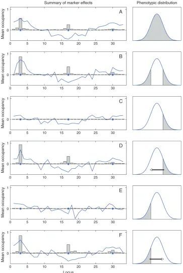
In Figure 3, A–F, the QTL occupancy probability (bars) and the mean standardized QTL effect (curve) summarize the QTL evidence at each locus over the 100 repetitions. Note that the same scales of the y-axis are used throughout. As expected, the analyses without doing any correction for truncated data performed very badly, showing practically no signals (Figure 3, C and E). It becomes evident from the graphs that the single-tail sampling analyses with pseudoobservations (Figure 3, D and F) have clearly more power than the analyses based on random subdata samples (Figure 3A) or the analyses that do not utilize the pseudoobservations (Figure 3, C and E). This is in the sense that analyses (Figure 3, D and F) on average show higher or elevated signals (QTL occupancy probabilities) around the true positions (3, 17, and 30). Surprisingly, in the case of the unlinked QTL, one can even conclude that the single-tail sam-pling analyses with pseudoobservations (Figure 3, D and F) showed power comparable to the analysis with two-tail sampling (Figure 3B). On the other hand, the mean of the estimated standardized effect size is practically at the same level in most of the analyses, which indicates that standardized effects seem to be (on average) com-parable across the different analyses. In Figure 3, D and F, note the negligible bias of the QTL position (around locus 17) in the opposite direction from the direction of sampling. The simulated effect size at position 30 was apparently very small because the position (on average) stayed undetected in most of the cases.

Heritability estimation: In schemes A–F in Table 1, the posterior mean heritability was estimated using the formulah2 _1=rPr

t¼1

s2ðtÞ

y s2

ðtÞ

e

=s2ðtÞ

y

;where

s2ðtÞ

y is the empirical phenotypic variance (from

aug-mented data in D and F),s2ðtÞ

e is the residual variance at

negative values arise because the residual variance was not restricted in the prior to be smaller than the phenotypic variance.) On the other hand, the heritabil-ity was overestimated in most of the analyses and the sampling variance was relatively small for analyses using single- or two-tail sampling (schemes B, D, and F) and pseudoobservations.

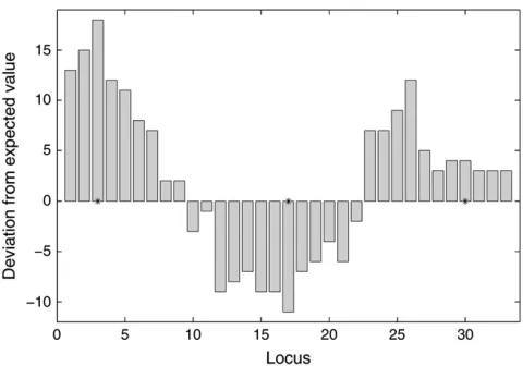
To enable comparison to more traditional methods (based on hypothesis testing) and to obtain an

under-standing of their potential performance on these data, Figure 4 shows the deviation of the marker genotype frequencies from their expected values in a typical real-ization of the data after right-tail sampling. One can clearly see the dependence of the frequencies over linked loci and the potential difficulty to control false positives by choosing the significance threshold. By looking at these data, it is easy to understand also the value of the multiple-QTL model.

Figure3.—Unlinked QTL: 100

data sets. (A–F) The posterior QTL occupancy probabilityPj

ð0:1Þ

¼ 1

100

P100

r¼1Pðjujj.0:1jdatarÞ

(indi-cated with a bar at each marker lo-cusj) averaged over 100 subdata analyses in the different samp-ling schemes. The corresponding mean of the standardized effect (calculated only over such MCMC rounds wherejujj.0.1) is shown

SIMULATION ANALYSIS OF TWO LINKED QTL

Simulated data:A base population of 2500 backcross individuals was generated using the QTL Cartographer software (Basten et al. 1996). Each individual had a single chromosome with 33 linked loci every 1 cM. Two closely linked QTL (in coupling and 14 cM apart from each other) were placed at 12 and 26 cM with additive genetic effectsb12¼1 andb26¼1, respectively. Only 11 markers (at 1, 4, 7, 10, 13, 16, 19, 22, 25, 28, and 31 cM) of the original 33 were included in the offspring data used in the analysis step.

We sampled 50 data replicates of size 1000 from the base population. For each replicate, a quantitative pheno-typey(i) was generated using the additive genetic model

yðiÞ ¼b₁₂1fg12ðiÞ¼ABg1b261fg26ðiÞ¼ABg1eðiÞ; ð6Þ

where the indicator functions 1fg12ðiÞ¼ABgand 1fg26ðiÞ¼ABg take value 1 only if individual i has genotype AB at positions 12 and 26, respectively. The additive errore(i) was generated from the standard normal distribution. This resulted in a heritability value0.47. Also, here no missing values were introduced into the marker data.

Analyses: For each of the 50 data replicates, subdata were sampled from the phenotype distribution of the 1000 individuals according to the different sampling schemes. Again, the six different analyses were consid-ered: (A) the analysis using a random subdata sample, (B) the analysis using a sample from both left and right tails, (C) the analysis using the right-tail sample without doing any correction with respect to truncation, (D) the analysis using the right-tail sample with pseudoobser-vations, (E) the analysis using the left-tail sample only

without doing any correction with respect to truncation, and (F) the analysis using the left-tail sample with pseu-doobservations. The sample sizes used in analyses C–F varied in each repetition, with mean 170 in C and D and mean 172 in E and F. Therefore, as in the first simulation study, the size of the random sample (A) was chosen to equal the mean of the sample sizes of the left- and right-tail samples (rounded upward), which resulted in a sample size of 171. In the two-tail sampling analysis (B), we randomly sampled half of the individuals from both tails (rounded upward), which also resulted in a sample size of171. The use of a larger sample size in the simulation analysis with linked QTL was partly moti-vated by not including the QTL (loci 12 and 26) into the marker set used in the analyses.

Results: For each data replicate, a Matlab implemen-tation of the method was run for 20,000 MCMC cycles from which 2000 burn-in rounds were discarded and only every 10th sample was stored (thinning), resulting in 1800 effective MCMC samples. In Figure 5, A–F, the QTL occupancy probability (bars) and the mean stan-dardized effect (curve) over the 50 repetitions are shown at each locus for each of the sampling schemes. As expected, the QTL localization was clearly more diffi-cult for two linked QTL (Figure 5) than it was for the unlinked QTL (Figure 3). No QTL were found in analyses C and E in Figure 5. In analyses A, B, D, and F in Figure 5, all markers in the region 10–31 cM showed elevated QTL occupancy. Arguably, in all cases (Figure 5, A, B, D, and F), the average QTL occupancy increased clearly at the flanking markers, at 10 and 13 cM and at 25 and 28 cM and showed the highest value at the marker closest to the QTL. One can conclude that in the case of two linked QTL, the single-tail sampling analyses with pseudoobservations (Figure 5, D and F) showed power

TABLE 1 Heritability estimates

Unlinked QTL Linked QTL

Sampling

scheme Mean

Standard

deviation Mean

Standard deviation

h2 _{0.50 0.47}

A 0.34 0.170 0.45 0.062

B 0.72 0.093 0.82 0.045

C 0.03 0.045 0.01 0.018

D 0.68 0.091 0.68 0.044

E 0.02 0.065 0.01 0.005

F 0.64 0.072 0.67 0.033

The mean value and the standard deviation of the heritability point estimates (posterior mean) were calculated, respectively, over 100 and 50 subdata analyses for the unlinked QTL and the linked QTL (in coupling) in the different sampling schemes (A–F). The simulated mean true heritability (h2_{), the analysis}

of the random subdata sample (A), the two-tail sample analysis (B), the direct and the mirror analysis of the sample from the right tail of the phenotype distribution (C and D), and the di-rect and the mirror analysis of the sample from the left tail of the phenotype distribution (E and F) are shown.

Figure4.—Unlinked QTL: a typical realization of the data

roughly comparable to the analysis with two-tail sam-pling (Figure 5B). Further, the power for the analyses using pseudoobservations (Figure 5, D and F) was clearly better than that for the analyses that did not utilize pseudoobservations (Figure 5, C and E), but it was only slightly better than that for the analyses based on random subdata samples (Figure 5A).

Heritability estimation:The mean value and the stan-dard deviation of the posterior mean heritability

calcu-lated over the 50 repetitions of the linked QTL data are shown for all six sampling schemes (A–F) in Table 1. As earlier, the random-sampling analysis (A) resulted in (on average) small heritability estimates and in large standard deviation (sampling variance). Also, negligible (or negative) heritability estimates were obtained in the analyses that used single-tail sampling without doing any correction with respect to truncation (C and E). Again, the analyses with single- or two-tail sampling and data

Figure_{5.—Linked QTL in}

cou-pling: 50 data sets. (A–F) The pos-terior QTL occupancy probability Pj

ð0:1Þ

¼ 1

50

P50

r¼1Pðjujj.0:1jdata

rÞ (indicated with a bar at each marker locusj) averaged over 50 subdata analyses in the different sampling schemes. The corre-sponding mean of the standard-ized effect (calculated only over MCMC rounds wherejujj .0.1)

augmentation (B, D, and F) produced overestimated heritabilities with small standard deviations. The over-estimation was highest for the two-tail sampling analysis (B). The most probable reason for the smaller standard deviations here (for linked QTL) compared to the case of unlinked QTL is that we used a larger sample size and a smaller number of repetitions.

Two linked QTL in repulsion (h2 _{0.1): For} com-parison, we also simulated five replicates of two linked QTL (in repulsion and placed on positions at 12 and 26 cM) with additive genetic effectsb₁₂¼ 1 andb₂₆¼

1, respectively. The heritability was0.10. The same six schemes of sampling from the phenotype distribution were again considered for each data replicate. Also, here each analysis was run for 20,000 MCMC rounds, which resulted in 1800 effective MCMC samples (after burn-in and thinning). Any notable difference were not found in the results when compared to the case of QTL in coupling. As earlier, the flanking markers showed elevated QTL occupancy in analyses B, D, and F. The QTL evidence was notably smaller in analysis A and no QTL were found in analyses C and E. In Figure 6 (left), the QTL occupancy probabilities (bars) and the un-standardized effect estimates (curve) are shown for one of the data replicates (heritability 0.10); the scale of the y-axis differs from the others in Figure 6B. In Table 2, for the same data replicate, the estimated posterior means and 90% credible intervals are shown for the heritabil-ities and the unstandardized and standardized QTL effects (for analyses B, D, and F) at the loci with highest QTL occupancy. Note that the effect estimates of ana-lyses D and F are surprisingly close to their true simu-lated values while in B they are clearly overestimated. However, the QTL were not exactly at the markers, which may partly downweight the estimates. The poste-rior mean heritabilities are highly overestimated in analyses B, D, and F but the true heritability value falls inside the 90% credible interval in all cases. In Table 2, the fact that the credible interval of the QTL effect includes zero is an indication of a somewhat lower QTL occupancy at the locus and therefore downward weight-ing of the estimate. In general, these kinds of model-averaged estimates are shown to be robust to upward bias of small-effect QTL (see Ball2001).

Two linked QTL in coupling (two realistic scenar-ios): To closely monitor performance of our method under a realistic single realization of a data set with large sample size and small heritability, we simulated two ad-ditional data sets, with the two linked QTL (in coupling and again placed on positions 12 and 26 cM) in each. The first data set has additive genetic effectsb12¼0.5 andb26¼0.2, and the second set hasb12¼0.6 andb26¼ 0.3, respectively. The heritabilities for the two sets were0.11 and 0.15. The same six schemes of sampling from the phenotype distribution were considered for both data sets. All analyses were based on 20,000 MCMC rounds and 1800 effective MCMC samples (after burn-in

and thinning). We first sampled 1000 and 1500 individ-uals from 2500, which was the size of the base popula-tion. The sample size in the first data set (subdata) was 162 for the left-tail sample and 161 for the right-tail sample, and in the second data set it was 232 for both the left- and the right-tail samples. Comparable sample sizes were used in other schemes. The QTL occupancy proba-bilities (bars) and the unstandardized effect estimates (curve) are shown in Figure 6 (center column) for the first data set (heritability 0.11) and in Figure 6 (right column) for the second data set (heritability 0.15); the scale of they-axis differs from the others in Figure 6B on the right. See Table 3 for the estimated posterior means and 90% credible intervals for the heritabilities.

In Figure 6 (center column), the flanking markers showed the highest QTL occupancy probabilities for one of the simulated QTL in analyses A and B, but the other QTL was undetected. In analyses C and E, all loci produced zero QTL occupancy probabilities. In analy-ses D and F, the loci around simulated QTL gained elevated QTL occupancy probabilities but the highest QTL occupancy probability was not necessarily obtained for the flanking markers. In Figure 6 (right column), one of the flanking markers showed the elevated QTL occupancy probability around one of the simulated QTL in A and around both QTL in B. In contrast to E, the analysis C also showed some elevated QTL occu-pancy probabilities. Again in analyses D and F, the loci around simulated QTL gained elevated QTL occupancy probabilities but the highest peaks did not necessarily occur at the flanking markers. To conclude the results of mirroring analyses D and F (Figure 6, center and right columns), it seems that the position estimates can be somewhat biased in the presence of two closely linked QTL and small heritability.

The heritabilities were badly overestimated with these data in analyses B, D, and F and the true heritability falls outside the 90% credible interval in all cases (Table 3).

SURVIVAL DATA ANALYSIS

Real mice data: We selected survival data of

autosomes in the QTL mapping (Bromanet al.2006). Also, the last marker at chromosome 19 was omitted from the mapping panel because it contained a large proportion of missing values. For simplicity we treated partial genotype information as completely missing here. Analyses: We analyzed the mice data using three different methods: (I) the Bayesian multiple-QTL ana-lysis with only those mice that died without generating pseudoobservations; (II) the Bayesian multiple-QTL

analysis with only those mice that died (with generating pseudoobservations and using the highest noncensored phenotype asT); and (III) the Bayesian multiple-QTL analysis with all 116 mice, using data augmentation to impute phenotypes (liabilities) for the censored mice withT¼log(264). Analysis I was carried out using our implementation of Xu (2003); see details from Hoti and Sillanpa¨ a¨(2006). Analyses II and III were carried out using the approach presented in themodelsection.

Figure 6.—Analyses of single

realizations: linked QTL in repul-sion,h2_{0.10 (left); linked QTL}

in coupling, h2 _{0.11 (center);}

and linked QTL in coupling, h2_{0.15 (right). (A–F) The}

poste-rior QTL occupancy probabilities P(jujj. 0.1 j data) estimated at

Note that approach III is in spirit similar to the one proposed for Gaussian mixed-effects models by S or-ensen et al. (1998). In all analyses, we adopted the F2transition probabilitiesp(Mio;jjM

o

i;j1) as presented in Sillanpa¨ a¨and Arjas(1998).

Results: The Matlab implementation of the method was run for 30,000 MCMC cycles. The first 15,000 rounds were discarded as burn-in and of the remaining samples only every 10th sample was used in the estima-tion. For the F2 design, at marker j, bj,1 ¼ 0 for het-erozygotes and the standardized effect fork¼{2, 3} is obtained asu_j;k¼bj;k3sˆj;k=sˆy;where ˆsj;kis the

empir-ical standard deviation of the indicator 1fms

i;j¼kg;and ˆsyis

the empirical standard deviation of the phenotype (cal-culated from augmented data in II and III). The pos-terior QTL occupancy probabilitiesP(juj,kj.0.1jdata) are separately calculated for k ¼ {2, 3} over

chromo-somes. In Figure 7, only the maximum of the two, max½P(juj,2j.0.1jdata),P(juj,3j.0.1jdata), is shown at each positionjfor the three different methods. Our results closely agree with the results by Broman(2003) who found QTL in chromosomes 1, 5, 13, and 15 using a single-QTL model. As in Broman(2003), our analyses support the conclusion that the QTL on chromosome 1 has an effect on the time to death only among the non-survivors (a peak is present only in analysis I). Similarly, QTL on chromosome 5 appear to have an effect only on the change of survival (a peak is present more or less only in analyses II and III). Again consistently with Broman(2003), QTL on chromosomes 13 and 15 have an effect on both (on the time to death among the non-survivors and on the change of survival; a peak is present more or less in all the analyses), where the latter chro-mosome actually has a weak QTL. In contrast to Diao et al. (2004), we did not find any QTL evidence on chromosome 6. However, a little support for QTL (with an effect only on the change of survival) was found on chromosomes 12 and 18 in analyses II and III, respec-tively. This may indicate higher efficiency in detecting QTL by our multiple-QTL analysis.

Heritability estimates:Bayesian point estimates (pos-terior means) of the heritability for analyses I, II, and III were 0.32, 0.49, and 0.41, respectively. The correspond-ing 90% credible intervals were½0.09, 0.50,½0.34, 0.61, and½0.25, 0.57.

DISCUSSION

In the consideration of the single-tail problem it is important to make a clear distinction between the phe-notype distribution and the conditional phephe-notype distribution (i.e., phenotype after correcting for QTL). In principle it is possible to use a truncated normal distribution function as an incomplete-data likelihood

TABLE 2

Posterior estimates of the heritability and the QTL effects

QTL effects

Sampling scheme Heritability estimate Locus Unstandardized Standardized

h2 _0.10

A 0.01½0.19, 0.19 13 1.95½2.60,1.29 0.58½0.77,0.38

B 0.16½0.01, 0.31 25 1.31½0.00, 2.22 0.39½0.00, 0.66

C 0.01½0.21, 0.16 13 0.93½1.17,0.69 0.62½0.76,0.48

D 0.22½0.10, 0.33 25 0.84½0.61, 1.07 0.56½0.42, 0.70

E 0.02½0.23, 0.16 13 0.72½1.09, 0.00 0.47½0.69, 0.00

F 0.22½0.10, 0.33 28 0.85½0.58, 1.09 0.55½0.39, 0.70

The heritability (posterior mean as a point estimate and 90% credible interval) and the unstandardized and standardized QTL effects (posterior mean and 90% credible interval) from the subdata analysis of the linked QTL (in repulsion) in the different sampling schemes (A–F) are shown. The estimates are based on the whole MCMC sample after burn-in (no thinning). Simulated true heritability (h2_{), the analysis of the random subdata}

sample (A), two-tail sample analysis (B), the direct and the mirror analysis of the sample from the right tail of the phenotype distribution (C and D), and the direct and the mirror analysis of the sample from the left tail of the phenotype distribution (E and F) are shown.

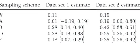
TABLE 3 Heritability estimates

Sampling scheme Data set 1 estimate Data set 2 estimate

h2 _{0.11 0.15}

A 0.01½0.19, 0.19 0.19½0.06, 0.30 B 0.28½0.14, 0.40 0.42½0.33, 0.51 D 0.28½0.18, 0.38 0.35½0.26, 0.42 F 0.18½0.07, 0.29 0.35½0.26, 0.42

The estimated heritabilities (posterior mean and 90% cred-ible interval) from two subdata analyses of the linked QTL (in coupling) in the different sampling schemes (A, B, D, and F) are shown. The estimates are based on the whole MCMC sam-ple after burn-in (no thinning). Simulated true heritability (h2_{), the analysis of the random subdata sample (A), two-tail}

for a single-tail sample in a way similar to that of Carriquiryet al. (1987); see also Schmeeand Hahn (1979). However, these expressions are difficult to deal with analytically, which means that the fully conditional posterior distributions are not available (Sorensenet al. 1998). Also such a model is very sensitive to small val-ues of the trait (Coxand Oakes1984). In contrast, the MCMC sampling distributions concerning QTL model parameters are unaffected by correction in correction methods based on a nontruncated normal distribution as full-data likelihood. Following the latter, we have presented a new method that can be applied together with a multiple-QTL model to improve the efficiency of QTL mapping using single-tail samples. The method effectively utilizes additional information available from the parents in the data augmentation scheme. This is

done by generating artificial sample points with the genotypes obtained deductively from the parental mating type and the phenotypes via data augmentation. Generally, the use of data augmentation and missing-data imputation is very common in Bayesian analyses (e.g., Albert and Chib 1993; Sillanpa¨ a¨ and Arjas 1998; Sorensenet al.1998; Bakeret al.2005). Note that, unlike methods that rely on the Mendelian inheritance assumption, this method can be applied to fitness traits, to loci that are associated with the survival to birth, and to loci that suffer from segregation distortion. When mapping viability (selection) in F2/outbred popula-tions, both the selection intensity and the dominance can be estimated.

Different QTL models and designs:The performance of the method was demonstrated using a multiple-QTL

Figure 7.—Survival data analysis: the

model where only markers (or pseudomarkers) were considered as putative QTL positions (e.g., Xu 2003). However, the presented data augmentation for hidden observations can in principle be applied together with the majority of the existing Bayesian QTL mapping meth-ods for inbred line-cross data, including interval mapping (e.g., Sillanpa¨ a¨ and Arjas 1998) and epistatic models (e.g., Yiand Xu2002; Yiet al.2003; Zhangand Xu2005). It can also be added to Bayesian models that consider outbred line-cross (e.g., Sillanpa¨ a¨ and Arjas1999) or outbred family/trio data (e.g., Leeand Thomas 2000), given the known or estimated haplotypes in parents. Recall the generality of Figure 1 in generating mirror images of the genotype data. The computational feasibility of each extension depends on the available computer capacity and on the complexity of the model considered. In binary traits, the pseudocontrol sample (based on parental data) can be created directly and analyzed with standard QTL/ association mapping methods and software packages designed for binary trait locus/association mapping (e.g., Xu and Atchley 1996; Visscher et al. 1996; Yi and Xu2000; Kilpikariand Sillanpa¨ a¨2003; Sillanpa¨ a¨ and Bhattacharjee2005), by assuming that there are no missing marker data. In a frequentist setting, one may try to pursue the implementation of the presented method for quantitative traits by using the EM algorithm (Dempsteret al.1977; Pettitt1986; Smithand Helms 1995). The underlying key assumptions made in the mirroring approach for quantitative traits are (1) given haplotypes for parents, the genotype data of the hidden observations are made to be maximally dissimilar to the observed data and (2) conditionally on genotypes, all updated (predicted) phenotypes for the hidden obser-vations are either on the left or on the right side of the truncation point and the observed phenotypes. Note that these assumptions correspond to assuming that observa-tions can be (in the light of the current genetic model) divided into two ordered parts: All hidden phenotypes are smaller (or greater) than the observed phenotypes. However, this assumption (see themodelsection) does not directly rule out certain genetic models;e.g., for an additive multiple-QTL model, it imposes a constraint for the sum of the QTL effects rather than restricting each QTL individually. Similar kinds of assumption (for liabili-ties) are also needed for discrete/binary phenotypes in the case of a multiple-QTL model. Such assumptions do not exclude us from using, for example, epistatic QTL models in mapping but it would be valuable to assess the limitations and possible negative influences of these assumptions for several model types in the future.

Mapping selection in breeding populations by using single-parent data:Gomez-Rayaet al.(2002) proposed the method to find the loci responsible for artificial or natural selection on the basis of testing distorted seg-regation among selected and nonselected offspring or gametes (obtained by single-sperm typing) of widely used bulls in cattle. As stated in Goddard(2003), this

method shows significant departure from the expected 1:1 ratio for two sire alleles, when measured from the selected offspring or gametes, at a locus linked to the selection. Utilization of the pseudoobservation and data augmentation scheme (for quantitative traits) together with this kind of design is also possible. As an advantage, a multiple-QTL model can be applied. Let us assume that our data consist of a small number of sires and their offspring groups, where each sire has a large number of offspring. Let us then assume that only selected off-spring (with phenotype value y¼ 1 or a tail-sampled quantitative phenotype) from each sire group are geno-typed. Again to form the complete mapping population, ungenotyped individuals can now be generated by applying the pseudoobservation idea. For a heterozy-gote sireAB, the pseudoobservation corresponding to the offspring genotypeA* isB* and vice versa. (Here * indicates the other/maternal allele.)

in the position estimates of two linked QTL, one could estimate the locations from the full data set where also the phenotypes of the ungenotyped individuals, if avail-able, are included (Roninet al.1998).

Efficiency of the sampling:Selective genotyping, two-tail sampling from the phenotype distribution, has been suggested as a ‘‘state-of-the-art’’ sampling scheme to im-prove the power of the analysis (Landerand Botstein 1989; Darvasi and Soller 1992; Sen et al. 2005). In our simulation analyses, we were able to demonstrate comparable power using data resulting from single-tail sampling. (Improvement of the power by generating pseudoobservations for two-tail sampled data is an open question that needs to be studied in the future.) However, it is well known that the power of any selection scheme depends on the underlying genetic architecture of the trait. Due to this, the two-tail sampling approach may lead to an unexpected drop of power, for example, in the presence of epistatic interactions (see Allison et al.1998). Also, if the QTL effects are small, selective genotyping does not adversely affect the detection of epistasis (Senet al.2005). The same is evidently true for the single-tail sampling approach. On the other hand, in a number of situations it is possible to obtain data from a single-tail sample only, for example, if the cross-ing experiments suffer from the lethal effects of in-breeding depression, in which case our method may prove to be an irreplaceable tool.

Survival data:Finally, we briefly comment on analyz-ing survival data with our method. Diao et al. (2004) analyzed censored observations by using parametric proportional hazard models and Broman(2003) used a mixture model for the same purpose. Both methods assumed that genotype data have been observed from all the individuals. Additionally, Broman (2003) as-sumed that the censoring time is equal among all the study subjects. We made the same assumption in our analysis above. In our method, it is possible to relax both of these assumptions. To account for individual-specific censoring times Ti, Equation 2 becomes ‘‘yih#Ti#yoi

for all pairsi,’’ and the hidden observations are updated by the Gibbs sampling distribution where each individ-ual has its own truncation point (step 4 in parameter estimation). A Matlab implementation of the method is available from the authors upon request.

We are grateful to Karl Broman for his comments on theListeria monocytogenesdata and to two anonymous referees for their construc-tive comments on the manuscript. This work was supported by a research grant (no. 202324) from the Academy of Finland.

LITERATURE CITED

Albert, J. H., and S. Chib, 1993 Bayesian analysis of binary and

polychotomous response data. J. Am. Stat. Assoc.88:669–679. Allison, D. B., N. L. Schork, S. L. Wong and R. C. Elston,

1998 Extreme selection strategies in gene mapping studies of oligogenic quantitative traits do not always increase power. Hum. Hered.15:261–267.

Baker, P., K. Mengersenand G. Davis, 2005 A Bayesian solution to

reconstructing centrally censored distributions. J. Agric. Biol. Environ. Soc.10:61–84.

Ball, R. D., 2001 Bayesian methods for quantitative trait loci

map-ping based on model selection; approximate analysis using the Bayesian information criterion. Genetics159:1351–1364. Basten, C. J., B. S. Weirand Z.-B. Zeng, 1996 QTL Cartographer, the

Reference Manual and Tutorial for QTL Mapping.North Carolina State University, Raleigh, NC.

Beasley_{, T. M., D. Y}ang_{, N. Y}i_{, D. C. B}ullard_{, E. L. T}ravis_{et al.,}

2004 Joint tests for quantitative trait loci in experimental crosses. Genet. Sel. Evol.36:601–619.

Beavis_{, W. D., 1998 QTL analyses: power, precision, and accuracy,}

pp. 145–162 inMolecular Dissection of Complex Traits, edited by A. H. Paterson. CRC Press, Boca Raton, FL.

Boyartchuk, V. L., K. W. Broman, R. E. Mosher, S. E. F. D’Orazio,

M. N. Starnback et al., 2001 Multigenic control of Listeria monocytogenessusceptibility in mice. Nat. Genet.27:259–260. Broman, K. W., 2003 Mapping quantitative trait loci in the case of

a spike in the phenotype distribution. Genetics163:1169–1175. Broman, K. W., and T. P. Speed, 2002 A model selection approach

for identification of quantitative trait loci in experimental crosses. J. R. Stat. Soc. B64:641–656.

Broman, K. W., S. Sen, S. E. Owen, A. Manichaikul, E. M. Southard

-Smithet al., 2006 The X chromosome in quantitative trait locus

mapping. Genetics174:2151–2158.

Carbonell, E. A., M. J. Asins, M. Baselga, E. Balansardand T. M.

Gerig_{, 1993 Power studies in the estimation of genetic}

param-eters and the localization of quantitative trait loci for backcross and doubled haploid populations. Theor. Appl. Genet. 86:

411–416.

Carriquiry, A. L., D. Gianolaand R. L. Fernando, 1987

Mixed-model analysis of a censored normal distribution with reference to animal breeding. Biometrics43:929–939.

Casella, G., and E. I. George, 1992 Explaining the Gibbs sampler.

Am. Stat.46:167–174.

Chib, S., and E. Greenberg, 1995 Understanding the

Metropolis-Hastings algorithm. Am. Stat.49:327–335.

Clayton, D., 2003 Conditional likelihood inference under complex

ascertainment using data augmentation. Biometrika90:976–981. Cox_{, D. R., and D. O}akes_{, 1984 Analysis of Survival Data.Chapman}

& Hall, London.

Darvasi_{, A., 1997 The effect of selective genotyping on QTL}

map-ping accuracy. Mamm. Genome8:67–68.

Darvasi_{, A., and M. S}oller_{, 1992 Selective genotyping for}

deter-mining of linkage between a marker locus and a quantitative trait locus. Theor. Appl. Genet.85:353–359.

Dempster_{, A. P., N. M. L}aird_{and D. B. R}ubin_{, 1977 Maximum}

like-lihood from incomplete data via the EM algorithm. J. R. Stat. Soc. B39:1–38.

Devroye_{, L., 1986 Non-Uniform Random Variable Generation.}

Springer-Verlag, New York.

Diao_{, G., D. Y. L}in_{and F. Z}ou_{, 2004 Mapping quantitative trait loci}

with censored observations. Genetics168:1689–1698.

Falk_{, C. T., and P. R}ubinstein_{, 1987 Haplotype relative risks: an}

easy reliable way to construct a proper control sample for risk cal-culations. Ann. Hum. Genet.51:227–233.

Feenstra_{, B., and I. M. S}kovgaard_{, 2004 A quantitative trait locus}

mixture model that avoids spurious LOD score peaks. Genetics

167:959–965.

Fu, J., and R. C. Jansen, 2006 Optimal design and analysis of genetic

studies on gene expression. Genetics172:1993–1999.

Gauderman_{, W. J., J. S. W}itte_{and D. C. T}homas_{, 1999 Family-based}

association studies. J. Natl. Cancer Inst. Monogr.26:31–37. Greenland_{, S., 1999 A unified approach to the analysis of}

case-distribution (case-only) studies. Stat. Med.18:1–15.

Goddard_{, M. E., 2003 Detecting selection. Heredity90:277–277.}

Gomez-Raya, L., H. G. Olsen, F. Lingaas, H. Klungland, D. I. Va˚ ge et al., 2002 The use of genetic markers to measure genomic re-sponse to selection in livestock. Genetics162:1381–1388. Gru¨ newald, M., 2004 Genetic association studies with complex

as-certainment. Licentiate Thesis, Stockholm University, Stockholm. Henshall, J. M., and M. E. Goddard, 1999 Multiple-trait mapping