ABSTRACT
MUTHUKARUPPAN, VALLIAPPAN. Practical Aspects of Implementing a Decentralized Volt-VAR Optimization Scheme. (Under the direction of Dr. Mesut Baran).
This study investigates the practical aspects involved in implementing a decentralized
Volt/VAR control scheme on smart distribution networks with PV penetration.
The deployment of DER on power grids around the nation is happening much faster than
most experts expected just a few years ago, and the tools needed to adjust for the changes
in many cases do not yet exist. Penetration limits are often imposed due to the impact
these additional distributed resource can have on voltage. Multiple Research is undergoing
which proposes new methodologies and technologies that would enable the penetration of
high PV. One of such methodology is to develop distributed and decentralized Volt/VAR optimization schemes. But most of these studies are simulation based implemented on
small test systems which are not realistic. The development of technologies like Smart
Inverters, Solid State Transformers are very new to the utilities and usually they are
reluc-tant to implement these new devices without exhaustive research and tests. There hasn’t
been much research until recently on developing a platform that would help the utilities in
developing, implementing and testing these new technologies in a modular, scalable and
realistic manner.
In this thesis, multiple testbeds are developed using the futuristic software platform and
devices that would enable the utilities in designing and testing the Volt/VAR Optimization algorithms in a decentralized fashion. Various performance metrics are analyzed and the
VAR injection element will lead to a huge increase in number of Volt/VAR devices in the system. This also increases the communication requirements which are not already present
in the system. The main motivation of employing distributed and decentralized algorithms
is to ease the burden on the existing communication infrastructure which is studied by
analyzing the communication requirements for a IEEE-123 Node system with partial PV
© Copyright 2019 by Valliappan Muthukaruppan
Practical Aspects of Implementing a Decentralized Volt-VAR Optimization Scheme
by
Valliappan Muthukaruppan
A thesis submitted to the Graduate Faculty of North Carolina State University
in partial fulfillment of the requirements for the Degree of
Master of Science
Electrical Engineering
Raleigh, North Carolina
2019
APPROVED BY:
Dr. David Lubkeman Dr. Ning Lu
DEDICATION
To my parents,
Muthukaruppan Manickam and Latha Muthukaruppan
my sister,
Meena Sundaram
BIOGRAPHY
Valliappan Muthukaruppan was born in Tiruchirappalli, Tamil Nadu, India, in 1991. He
received his Bachelors’ degree in Electrical and Electronics Engineering from National
Institute of Technology Trichy, in 2014. From 2014 to 2016 he worked as a Senior Electrical
Engineer with Larsen & Toubro Ltd., Qatar where he was the lead erection engineer for the
132/11kV Doha Festival City Substation. The substation was successfully commissioned and energized in June, 2016.
In 2016 he joined North Carolina State university to pursue Master of Science in
Elec-trical Engineering. In 2017 he joined the FREEDM System Center as a research assistant
ACKNOWLEDGEMENTS
My sincere gratitude goes to the people who made this work possible.
To my advisor, Dr. Mesut E. Baran, who has continuously guided and encouraged me with
his insight and patience throughout the time I was at NC State University.
To my committee members, Dr. David Lubkeman and Dr. Ning Lu for their valuable time,
suggestions and help.
To my research fellows in the FREEDM System Center. It is a great pleasure to work with
you all. To my friends, Thomas Dotson & Semih Isik who have always been supportive and
helped me through my tough times.
And last and foremost, to my parents, Muthukaruppan & Latha, and my sister, Meena for
TABLE OF CONTENTS
LIST OF TABLES . . . vii
LIST OF FIGURES. . . viii
Chapter 1 INTRODUCTION. . . 1
1.1 Volt/Var Control on Conventional Systems . . . 1
1.1.1 Effect of PV Penetration . . . 3
1.2 Objectives of Volt/Var Control . . . 4
1.3 State of the Art Volt/VAR Control . . . 5
1.3.1 Smart Distribution System . . . 8
1.3.2 FREEDM Distribution System . . . 9
1.3.3 Motivation . . . 10
1.3.4 Decentralized Volt/VAR Optimization . . . 11
1.4 Proposed Work . . . 14
Chapter 2 Decentralized VVO using DGI . . . 15
2.1 Centralized DMS . . . 16
2.1.1 Centralized DMS Architecture . . . 16
2.1.2 State-of-the-art Centralized SCADA Platform . . . 19
2.2 DGI Overview . . . 20
2.2.1 DGI Architecture . . . 22
2.2.2 DGI Device Framework . . . 29
2.2.3 DGI Adapters . . . 30
2.3 Application Development in DGI . . . 33
Chapter 3 REAL-TIME IMPLEMENTATION . . . 36
3.1 Green Energy Hub (GEH) Testbed . . . 38
3.2 Large Scale System Simulation (LSSS) Testbed . . . 44
3.2.1 IEEE 34 Node System . . . 45
3.2.2 IEEE 123 Node System . . . 48
3.3 Hardware-in-loop (HIL) Testbed . . . 66
3.4 Conclusion . . . 67
Chapter 4 COMMUNICATION REQUIREMENT . . . 70
4.1 Smart Grid Communication . . . 71
4.2 Automatic Metering Infrastructure . . . 74
4.3 RF Mesh Systems for Smart Metering . . . 76
4.3.1 Architecture . . . 77
4.4 VVO using AMI Infrastructure . . . 80
4.4.1 Objective . . . 82
4.4.2 Location of Collectors . . . 82
4.5 Performance Assesment . . . 85
4.5.1 Scheme-I Volt/VAR Optimization . . . 89
4.5.2 Scheme-II Volt/VAR Optimization . . . 103
4.6 Conclusion . . . 114
Chapter 5 Conclusion and Future Work. . . 116
5.1 Conclusion . . . 116
5.2 Future Work . . . 117
LIST OF TABLES
Table 2.1 Comparision between Centralized DMS and DGI Architecture . . . 28
Table 2.2 Adapter types fully tested with DGI . . . 29
Table 3.1 Round Trip Time for Slave-1 . . . 39
Table 3.2 Metrics for Round Trip Time of Slave-1 . . . 40
Table 3.3 Round Trip Time for Slave-2 . . . 42
Table 3.4 Metrics for Round Trip Time of Slave-2 . . . 42
Table 3.5 Round Trip Time for Slave-3 . . . 43
Table 3.6 Metrics for Round Trip Time of Slave-3 . . . 43
Table 3.7 Nodes with PV system in 123 Node Feeder . . . 53
Table 3.8 Scheduled Time for DGI Applications . . . 57
Table 3.9 Data Rate from Wireshark for IEEE 123 Node LSSS . . . 59
Table 4.1 Best Case and Worst Case Throughput Degradation . . . 84
Table 4.2 Number of Smart Meters in the Circuit . . . 89
Table 4.3 Summary of Maximum Number of Hops and B.W. degradation in Scheme-I . . . 98
Table 4.4 Assumptions for data size calculation for Scheme-I . . . 101
Table 4.5 Computation of Time taken by Smart Meters in Scheme-I for commu-nication . . . 102
Table 4.6 Computation of Time taken by Collectors in Scheme-I for communi-cation . . . 103
Table 4.7 Number of Aggregators in the Circuit . . . 104
Table 4.8 Assumptions for data size calculation for Scheme-II . . . 112
Table 4.9 Computation of Time taken by Aggregators in Scheme-II for commu-nication . . . 113
LIST OF FIGURES
Figure 1.1 Without volt/Var Control under Light Load conditions . . . 2
Figure 1.2 Without volt/Var Control under Heavy Load conditions . . . 3
Figure 1.3 Effect of different levels of PV penetration on system Voltage Profile 4 Figure 1.4 State of the Art Volt/VAR Control . . . 7
Figure 1.5 Smart Distribution System of the future . . . 9
Figure 1.6 FREEDM System Configuration . . . 10
Figure 1.7 Two-level coordinated Volt/VAR control . . . 13
Figure 2.1 Architecture of the Decentralized VVO Scheme . . . 17
Figure 2.2 Centralized SCADA Architecture . . . 18
Figure 2.3 Centralized SCADA Architecture . . . 19
Figure 2.4 FREEDM Architecture with DGI . . . 21
Figure 2.5 Software Architecture of DGI . . . 23
Figure 2.6 Example of a DGI Phase-Sequence . . . 26
Figure 2.7 Communication between DGI and Device Server . . . 32
Figure 3.1 Hardware setup of GEH Testbed . . . 40
Figure 3.2 Communication Architecture of GEH . . . 41
Figure 3.3 LSSS setup . . . 46
Figure 3.4 Simple diagram of the FREEDM IEEE 34 Test System . . . 46
Figure 3.5 Grouping of SSTs in FREEDM IEEE 34 Node System . . . 48
Figure 3.6 24 hr Load Profile for the FREEDM 34 Node system . . . 49
Figure 3.7 Maximum Voltage in the FREEDM 34 Node System . . . 49
Figure 3.8 Minimum Voltage in the FREEDM 34 Node System . . . 50
Figure 3.9 Power Loss in the FREEDM 34 Node System . . . 50
Figure 3.10 Deviation from the Centralized Solution . . . 51
Figure 3.11 Delay in Communication for 34 Node System . . . 51
Figure 3.12 Simple Diagram of the IEEE 123 Test System . . . 52
Figure 3.13 FREEDM 123 System with location of PV nodes and grouping of slaves 54 Figure 3.14 24 hr Load Profile for the FREEDM 123 Node system . . . 55
Figure 3.15 Maximum Voltage in the FREEDM 123 Node system . . . 59
Figure 3.16 Minimum Voltage in the FREEDM 123 Node system . . . 60
Figure 3.17 Total Loss in the FREEDM 123 Node system . . . 60
Figure 3.18 Optimality of VVO for FREEDM 123 Node system . . . 61
Figure 3.19 Tap Position forV R1in the FREEDM 123 Node system . . . 61
Figure 3.20 Tap Position forV R2in the FREEDM 123 Node system . . . 62
Figure 3.21 Tap Position forV R3in the FREEDM 123 Node system . . . 62
Figure 3.22 Tap Position forV R4in the FREEDM 123 Node system . . . 63
Figure 3.24 Delay inQu p d a t e for the FREEDM 123 Node system . . . 64
Figure 3.25 Wireshark Capture Screenshot for 123-Node LSSS . . . 65
Figure 3.26 HIL: 24-hr Voltage Profile at Node 840 of the IEEE 34 Node system . . 69
Figure 3.27 HIL: Mapping of correctQc m d s to SSTs under Slave-6 . . . 69
Figure 4.1 Smart Grid Infrastructure . . . 72
Figure 4.2 Smart Grid Communication Infrastructure . . . 73
Figure 4.3 Smart Deployment in 2016, State-by-State . . . 74
Figure 4.4 General AMI Infrastructure . . . 76
Figure 4.5 RF Mesh System Architecture . . . 78
Figure 4.6 Sequence Hopping . . . 79
Figure 4.7 AMI based CVR . . . 81
Figure 4.8 Best Case Scenario . . . 83
Figure 4.9 Throughput Degradation in Multi-hop networks . . . 84
Figure 4.10 123 Node System With Partial PV Deployment . . . 87
Figure 4.11 Number of Smart Meters connected to each Node . . . 88
Figure 4.12 Location of Collectors in the System . . . 90
Figure 4.13 Group-1 for Scheme-I . . . 91
Figure 4.14 Group-2 for Scheme-I . . . 92
Figure 4.15 Group-3 for Scheme-I . . . 93
Figure 4.16 Group-4 for Scheme-I . . . 94
Figure 4.17 Group-5 for Scheme-I . . . 95
Figure 4.18 Group-6 for Scheme-I . . . 96
Figure 4.19 Maximum Number of Hops in Group-5 . . . 97
Figure 4.20 Load Aggregators for Scheme-II . . . 105
Figure 4.21 Group-1 for Scheme-II . . . 106
Figure 4.22 Group-2 for Scheme-II . . . 107
Figure 4.23 Group-3 for Scheme-II . . . 108
Figure 4.24 Group-4 for Scheme-II . . . 109
Figure 4.25 Group-5 for Scheme-II . . . 110
CHAPTER
1
INTRODUCTION
1.1
Volt
/
Var Control on Conventional Systems
Voltage control is fundamental requirement for an electric distribution system, as it is
the utility’s responsibility to keep the customer voltage within the specified tolerances
set by regulatory commissions[3].Conventional distribution systems are radial in nature, where substation is the only source of the feeder and the voltage along a feeder will drop
gradually from the substation towards the end of the feeder. Under heavy load conditions,
the nodes far away from the substation may have under-voltage violation as shown in
using Load Tap Changing (LTC) Transformers, as shown in Fig. 1.2. But this would cause
over-voltage violation under light load condition, especially on the nodes closer to the
substation. Sustained over-voltages or under-voltages can lead to inefficient equipment
operation at customer level and may even lead to tripping of sensitive loads. Hence, Volt/Var control schemes are needed to guarantee a desired system voltage profile under all possible
operating conditions. The most commonly used VVC devices on a conventional distribution
system are voltage regulators (VRs) and capacitor banks (CAPs).
Figure 1.2Without volt/Var Control under Heavy Load conditions
1.1.1
Effect of PV Penetration
Due to increasing penetration of distributed energy resources (DER) such as photovoltaic in
the distribution networks, the operating conditions (supply, demand, voltages, etc.) of the
distribution feeder fluctuates fast and by a large amount. The conventional voltage control
lacks flexibility to respond to these conditions and they may not produce the desired results.
This raises important issues on the network security and reliability. Fig. 1.3 shows the effect
of solar photovoltaics (PV) under different penetration level on the voltage profile of the
Distribution System. The variation in the voltage profile increases proportionally with the
Figure 1.3Effect of different levels of PV penetration on system Voltage Profile
Traditionally, distributed PV systems were installed with standard inverters that only inject
active power in to the grid. Recently, however, PV is increasingly being paired with smart
inverters that can also supply or absorb reactive power. With this ability to provide reactive
power, distributed PV has the potential to support and actively regulate local voltage and
power factor on the grid. Therefore, the Smart Inverters can provide reactive power to
com-pensate load and correct the power factor just as a shunt capacitor. But as compared with a
shunt capacitor, it can also provide reactive power with contiguous change to guarantee a
unity power factor.
1.2
Objectives of Volt
/
Var Control
As mentioned in section 1.1, the distribution system suffers from both over-voltage and
systems, voltage regulation is a fundamental operating requirement. Voltage regulation
brings added benefits including reducing power loss and energy loss. And it is always desired
to reduce power and energy loss in power distribution system for economic benefits. Thus,
reducing loss can be used as the secondary goal of Volt/Var control schemes. Both the Voltage regulators and Var support components like capacitors, SSTs, etc. aid in voltage
regulation and loss reduction simultaneously. Voltage regulation is more dominant in
Voltage regulators and loss reduction is more dominant in Var support devices. Hence, it
is necessary to coordinate the control of Var devices and voltage regulators to optimize
VAR flow while keeping voltages within limits[3].Some of the control objectives to this optimization problem include:
1. To meet power factor objectives at the substation
2. To regulate load voltages within set limits
3. To minimize energy losses
4. To minimize power losses
5. To minimize control cost
For the Volt/Var Optimization (VVO) Scheme adapted in this thesis the objective of the optimization problem is to minimize power loss while maintaining the voltages acceptable
under different system operating conditions.
1.3
State of the Art Volt
/
VAR Control
Volt/VAR device is communicated back to the Utility Control Center where an enterprise based Volt/VAR optimization algorithm runs. The optimal settings for the devices from the algorithm is then communicated back to the devices through the utilities communication
network.
Apart from keeping the voltage within limits, Utilities use centralized VVO schemes to
implement Conservation Voltage Reduction (CVR)[36, 39]. CVR allows the utility to reduce the peak demand in the network without shedding any loads. This method may fail in
the future due to increasing amount of Constant power loads like Electric Vehicles, LED
lights, etc. On the contrary the penetration of PV is increasing every year and as discussed
in section 1.1.1 this causes a lot of over-voltage and under-voltage violations in the circuit.
In the present scenario there is no way for the utility to understand the effect of these
DERs sitting behind the customers energy meters. There are no feasible way to forecast the
generation of these Distributed resources.
The revised IEEE 1547 standard for interconnection of DER has allowed for voltage
reg-ulation at the point of common coupling (PCC) by the PV inverters. With the increasing
penetration of DERs in distribution network, the industry is moving towards ability to
provide reactive power capability to the inverters but still it is not a common practice and
requires further revisions of the IEEE 1547 standard[17]. Once this is achieved then the number of inverters and hence the number of Volt/Var devices in the circuit will increase enormously. With the current centralized scheme and the communication infrastructure it
is not feasible to collect all the data from the Volt/VAR devices, run an optimization algo-rithm and dispatch control commands back to the devices within stringent time constraints.
voltage control in a smart distribution system have addressed this issue[4, 19, 29]. In[38] the author shows that the communication performance for voltage control of a distribution
circuit in UK having multiple distributed energy resources (DERs) implemented using a
cen-tralized scheme has high latency and communication duration to complete measurement
collection, control command delivery and coordination process compared to a distributed
scheme.
To address the above challenge a new concept of smart grid as the modern power grid
has emerged recently. The smart grid aims to address these issues using data processing,
networking, communications, sensor networks, automation and computational power.
1.3.1
Smart Distribution System
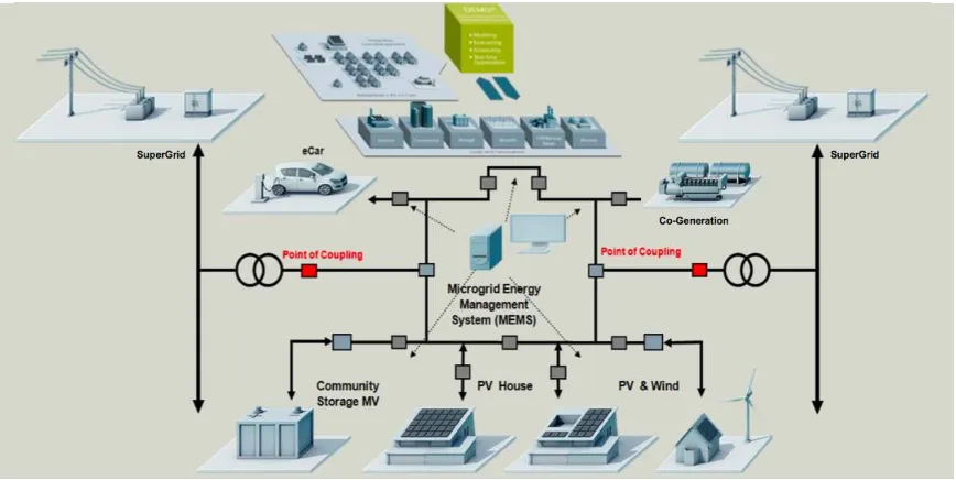
Fig. 1.5 shows the smart distribution of the future. Multiple energy resources like Solar, Wind,
Energy Storage Devices, Electric Vehicles will be part of the system. The smart grid address
the existing challenges in traditional grid like increasing complexity, economical operation,
growing demands, and requirements for greater reliability, security, efficiency,
environmen-tal and sustainability concerns using data processing, networking, communications, sensor
networks, automation and computational power. The concept of microgrids will play a
major role in the development of future smart grids. The use of microgrids can simplify
implementation of many smart grid functions like reliability, self-healing and load control
[20]. Microgrids can seemingly disconnect from the central grid and form a grid of their
own with local resources. To manage these resources microgrids usually run applications
in a distributed fashion among many Intelligent Energy Management (IEM) nodes. Hence,
when developing applications that control the overall system, it is necessary to implement
Figure 1.5Smart Distribution System of the future
1.3.2
FREEDM Distribution System
FREEDM (Future Renewable Electrical Energy Delivery and Management) is an
Engineer-ing Research Center (ERC) project supported by National Science Foundation (NSF)[10]. FREEDM distribution system is an example of smart grid with the main goals of enabling
plug-and-play renewable resources, energy storage, and implanting distributed intelligence
control, achieved by advanced technologies of renewable energy generation, energy storage,
solid state controller, and distributed intelligence control. It is a distributed system that
consists of multiple IEM nodes. Each node includes Solid State Transformer (SST),
Dis-tributed Renewable Energy Resource (DERS), DisDis-tributed Energy Storage Device (DESD),
and Distributed Grid Intelligence (DGI). DGI is a major cyber aspect in the FREEDM
sys-tem with each node running a portion of DGI within the intelligent Energy Management
utilization, storage and distribution over the smart grid.
Figure 1.6FREEDM System Configuration
All the Distribution System of interest in this thesis is considered to be a FREEDM
distribu-tion system and the Photovoltaics are assumed to be connected through a SST.
1.3.3
Motivation
• The centralized Volt/VAR control is implemented in the present scenario based on legacy devices like Voltage regulators & capacitor banks. These devices are owned
by the utility and can be easily integrated in to the Utilities communication network.
But the PV inverters or SSTs which will be majority of Volt/VAR devices in the future smart distribution system primarily installed behind the customer meter and utilities
donot have direct access to these devices for communication. A standard protocol
communication network with ease.
• It is evident that there is a strong necessity to move from a centralized algorithms to
decentralized algorithms. There are multiple research articles that have developed
distributed and decentralized algorithms for the existing centralized applications
like Energy Storage Management, Volt/VAR control but there isn’t any research that has studied the scalability of these algorithms in a realistic scenario. Many of these
distributed algorithms will be running parallely at each IEM node and it has to be
seen how the Volt/VAR control algorithm will perform in the presence of other local and distributed algorithms.
• Eventhough it is assumed that the decentralized algorithms would relieve the
com-munication burden on the network there hasn’t been many studies that explain the
communication infrastructure for implementing such algorithms in the existing
system and how far is the performance better from a centralized implementation.
1.3.4
Decentralized Volt/VAR Optimization
In[31]the author proposes a Master-Slave based Volt/VAR Control Scheme which addresses the following issues:
1. Heavy Communication Requirement for Centralized VVO schemes in systems with
large number of remote monitoring devices.
2. The size of a centralized VVO problem can be very large depending upon the number
of Volt/VAR devices in the system.
3. Smart distribution systems enable communication and processing capability at the
For a large distribution system with a great number of smart inverters or SSTs, the VVO
problem can be very large, which needs high computational efforts. In the adopted scheme
the large problem is decomposed in to smaller sub-problems in computationally efficient
way which is an important requirement of real-time implementation for smart distribution
systems.
1.4
Proposed Work
In Chapter-2 the software requirements for implementing a Decentralized Volt/VAR scheme and how DGI fulfills these requirements is discussed. The important components of DGI
and how it compares with a Centralized SCADA architecture is introduced. Finally, the
primary features that DGI offers to users for developing distributed and decentralized
applications is discussed in detail.
In Chapter-3 different testbeds that were utilized to implement the Decentralized Volt/VAR scheme are introduced and the advantage of each testbed from a utilities perspective is
discussed. Results of different circuit models implemented in these testbeds are shown to
analyze the performance of the scheme using DGI.
In Chapter-4 two schemes for implementing the proposed Volt/VAR scheme based on existing Automatic Metering Infrastrucutre (AMI) utilizing Multi-hop Radio Mesh Network
is discussed. Scheme-1 is based on the existing AMI infrastrucutre without any
modifica-tion while in scheme-2 the data from smart meters are consolidated at the distribumodifica-tion
transformer before being forwarded to the master. The communication performance of
these two scheme are compared and the best scheme for adopting Decentralized VVO is
CHAPTER
2
DECENTRALIZED VVO USING DGI
Fig. 2.1 shows the architecture of the decentralized VVO scheme adopted in this study. For
each group of SSTs, a VVO slave is assigned to collect the real-time monitoring data and to
forward the data to the VVO master at the substation. Each slave also receives data from
the master, determine the control commands for each SST in that group based on the data
received, and finally sends the control commands to SSTs.
While the master may or may not be located in the field, the slaves associated with the SSTs
are required to be distributed throughout the circuit. Furthermore, the VVO may not be
be running on the same slave. The slaves need to coordinate with each and the master in
real-time. Hence it is necessary to select a software architecture that enables peer-to-peer
communication as well as client-server based communication, distributed computation,
parallel processing and accommodates multiple applications using schedulers.
Conve-niently, DGI has all the above mentioned features and much more.
In this chapter, The state of the art centralized DMS architecture is discussed in brief and
utilized to introduce the DGI and its components. Then the important features and aspects
of DGI that would enable a user to develop distributed and decentralized algorithms are
discussed.
2.1
Centralized DMS
In a centralized DMS architecture, the field data and parameters for the whole system are
collected at a central location by using a Supervisory Control and Data Acquisition (SCADA)
system[15]. The information is then saved in a database and made available to a central controller (e.g.- computer) which runs the Volt-VAR optimization program to make the
control decision. Then, the decision is sent to the control devices like Voltage Regulators &
Capacitor banks in the system. The advantage of such a system is that the DMS has detailed
information about the whole system, which enables it to make optimal decision.
2.1.1
Centralized DMS Architecture
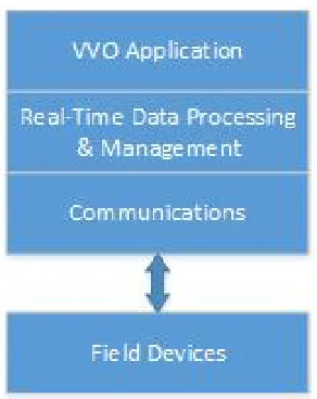
A generic software architecture for a traditional centralized SCADA/DMS is shown in fig-2.2. The basic building blocks can be identified as - communications, real time data processing
method in which each blocks utilizes the functionality provided by the layer below it &
provides service to the layer above it.
Figure 2.2Centralized SCADA Architecture
In a centralized SCADA/DMS system, the data from the field devices are collected at central location via communication channels. Power system specific communication protocols like
DNP3, IEC61850 are used for SCADA communications. The data is then processed and saved
to a historian for later retrieval. This process is part of the ’Real-Time Data Processing and
Management’ as shown in Fig. 2.2. Utility applications like Volt/VAR optimization, economic dispatch, load forecasting, etc. utilize the real-time and historical data to calculate set-points
for control devices in the field. The set-points are then dispatched via communication
2.1.2
State-of-the-art Centralized SCADA Platform
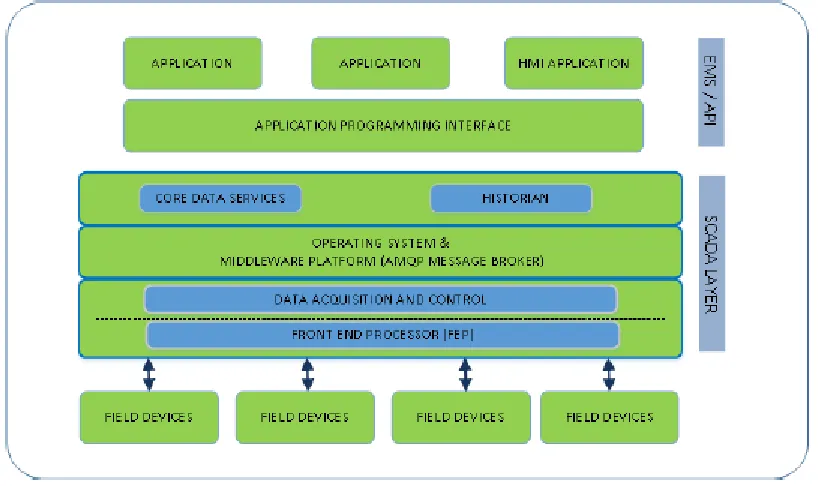
To understand the building blocks of a Centralized SCADA architecture, a state-of-the-art
SCADA platform called GreenBus system is studied in detail. The Fig. 2.3 below shows the
building blocks of the GreenBus SCADA in a stacked software architecture diagram.This
figure will be referred to when different aspects of the GreenBus software architecture will
be discussed.
Figure 2.3GreenBus SCADA Architecture
The architecture of the GreenBus SCADA system comprises of the following components
which is discussed in detail by the author in[15]:
1. Operating System (OS)
3. Front End Processor (FEP)
4. Core Data Services
5. Historian
6. Applications
7. Application Programming Interface (API)
2.2
DGI Overview
The FREEDM DGI is a distributed operating system developed to manage power and
com-putational resources within a smart microgrid, using the FREEDM system architecture as a
model (Fig. 1.6). The FREEDM system is managed by DGI that embodies the functions of
configuration management, power management, and fault detection, configuration and
reconfiguration. The DGI is a major computational aspect of the FREEDM system with
a portion of DGI running on a computer embedded in each IEM node managing energy
resources through the embedded SST. The overall FREEDM architecture with DGI is shown
in Fig. 2.4.
DGI consists of exhaustive features to implement distributed algorithms for power device
control in the smart grid:
1. Real-time scheduling for execution of distributed algorithms using an integrated
round-robin scheduler
2. Automatic detection and configuration for DGI processes. The DGI automatically
algorithms. Updates are pushed to each module on change.
3. Device management and integration with PSCAD and RSCAD/RTDS simulations
4. Physical devices can be easily integrated by implementing Plug n’ Play protocol
5. Casually consistent global snapshot capturing. This can be used to capture the state
of a smart grid using a method that compensates for latency.
2.2.1
DGI Architecture
Fig. 2.5 shows the software architecture of DGI. The architectural design of DGI is realized in
C++using the Boost Library. Other Languages such as Python are used to provide
bootstrap-ping and start-up routines for the software modules. In this section each component of the
architecture is discussed in detail and a resemblance is drawn in terms of functionality to
the corresponding component in Centralized DMS architecture.
2.2.1.1 State Collection
Even though State Collection (SC) is a software module, along with Group Management
(GM) forms an integral part of all the other software modules registered in the DGI. The state
of the DGI consists of the states of each IEM, their software modules, and any messages in
transit. The state collection is invoked when a consistent state of the system is required
(such as for Volt/VAR optimization). The Chandy-Lamport state collection algorithm is used to collect a logically consistent state (one in which causality between actions is preserved).
Modules submit requests to state collection, state collection in-turn runs those collections
during it’s phase (Fig. 2.6), and returns the collected state as a message to the requesting
Figure 2.5Software Architecture of DGI
2.2.1.2 Group Management
Group Management provides consistent list of active DGI processes as well as identifies a
primary process for initiating distributed algorithms. The group manager maintains the
state of the system regarding the status of each IEM node, active, disabled, requesting entry,
and requesting departure from the FREEDM system. In the event of IEM node failure or
complete system failure and recovery, the group manager collaborates with its peer IEM
nodes to reconstruct the FREEDM system using the Invitation Algorithm of Garcia-Molina.
This algorithm provides a robust election procedure which allows for transient partitions.
Transient partitions are formed when a faulty link inside a group of processes causes the
group to divide temporarily. These transient partitions merge when the link becomes more
grid.
Group Management will send all modules in the system aPeerListmessage when the list
of active processes in the system changes. This message will also contain the identity of
the leader process. Group Management provides a static method to aid processing this
message. Group management can be configured to respect the topology of the physical
network, meaning it will not group two DGI nodes unless physical path exists between the
two processes (as opposed to a cyber path).
2.2.1.3 Broker
The Broker is responsible for integrating plug-in software modules like group management,
state collection, power management and Volt/Var Optimization subsystem. It reflects the changes in the configuration of the FREEDM system inside power management and state
collection modules. The core components of Broker are:
1. POSIX Broker
2. CBroker
3. CDispatcher
4. Connection Manager
5. CMessage module
The broker runs as a process that manages individual POSIX threads which in turn invokes
the CBroker class that instantiates each software module as shown in Fig. 2.5. A connection
object tracks new and existing connections via the universally unique identifier (UUID)
generated uniquely per-host when first executed. This UUID allows the connection
man-ager to uniquely map connections to a specific peer node tracked in the group manman-ager.
This allows for nodes entering and leaving the network due to transient failures and initial
activation of the IEM to join an existing group. The individual connections are managed
by an event-triggered system that responds to message transmission, reception and
con-figurable timers. Each software module registers at run-time which types of messages it is
interested in sending and receiving. The CDispatcher class parses incoming messages and
dispatches them to the registered modules. Each message may contain more than one type
of sub-message, allowing the modules managed by the broker to interact in a coordinated
fashion. The incoming message is passed to the module’s message handlers in order that
they were registered during the start-up process. The CDispatcher also provides the option
for modules to handle outgoing messages, if needed. In all cases, the CDispatcher provides
a prioritized selection of messages and delivers them to their respective destinations, as
directed.
When a message is received for processing, it will be taken into the CListener module where
it is processed to determine if it should be accepted or rejected. If accepted, it is passed to
the dispatcher which examines the contents to determine which modules if any should
be given the message. The module responsible for receiving the message is immediately
called and allowed to act on the message.
Even though the phases proceed in a round robin fashion, there are some complications in
the implementation. Consider the example shown in Fig. 2.6:
Figure 2.6Example of a DGI Phase-Sequence
function, requests them to be sent and then idles.Send(), which is handled by the
broker operates outside of the module scheduler and begins work immediately.
2. Since group management has no work to do while waiting for replies, the system is
idle. (BetweenB&C)
3. C- Message(s) arrive from other DGI nodes in the system. Since one of them is
addressed to group management and the scheduler is currently in GM phase, the
worker immediately fulfills the request.
4. D- Processing the message makes GM over-run its phase.
5. A- There is a"No-man’s"land where the group management task is completing work
outside of its phase, but the scheduler is ready to switch phases to SC. Because GM
has the highest priority and all other modules are dependent on GM, SC is penalized
by the overflow.
6. A- The scheduler has changed phases, but the broker does work on a received message
queue for its intended process, so the message processing time is only spent by the
Broker and communication stack.
7. E- Finally, the SC module begins.
2.2.1.4 Scheduler
The Scheduler performs real-time scheduling for execution of distributed algorithms. The
real time scheduler uses a round robin approach. A module’s individual processing time is
defined as it’s"Phase". A typical round is composed of GM (Group Management) Phase, a SC
(State Collection) Phase, a LB (Load Balancing) Phase and a VVO (Volt/VAR Optimization) Phase. Every DGI instance must have the same timing profile.
2.2.1.5 Communication Protocol
Several of the distributed algorithms developed in DGI require the use of ordered
commu-nication channels. To achieve this, FREEDM provides a reliable ordered communicaiton
protocol (SRC - Sequenced Reliable Connection) to the modules, as well as a "best effort"
protocol (SUC - Sequenced Unreliable Connection) which is also a FIFO (First In, First Out)
architecture but provides limited delivery guarantees.
2.2.1.6 Centralized DMS vs. DGI
Table 2.1 summarizes the resemblance between the components of Centralized DMS and
Table 2.1Comparision between Centralized DMS and DGI Architecture
Sl. No. Centralized DMS DGI
1 Front End Processor (FEP) CMessage+ConnectionManager+ CConnection
2 Advanced Message Queuing
Protocol (AMQP) CDispatcher+PosixBroker+CBroker
3 Core Data Services No specific Storage of Data, Data directly addressed to software modules
4 Historian No component in DGI with Similar
functionality
5 Application Programming
Interface (API) Individual Module’s Message Handlers
6 Applications Software Modules
2.2.2
DGI Device Framework
The DGI supports interaction with physical devices such as SSTs and DESDs through its
device framework. This framework can communicate with both simulated and real devices.
An important distinction is that this communication framework is independent of the
protocol used to communicate with other DGI Instances.
All the devices used by the DGI must be defined in thedevice.xmlconfiguration file located
inside the Broker. If a device is not specified in this file, then the DGI cannot communicate
with it.
The communication protocol that the DGI uses to communicate with its physical devices
depends on the type of physical adapter configured to run with the DGI. For most cases,
configuration of the DGI physical adapters requires modification of theadapter.xml
config-uration file also located inside the Broker. The adapter files fully tested with DGI are shown
in 2.2
Table 2.2Adapter types fully tested with DGI
Adapter Type Communication Protocol Communicates With
rtds TCP/IP RTDS/PSCAD Simulators
pnp TCP/IP Physical Hardware
fake none nothing
CDeviceManager is the interface between broker modules and the device architecture.
a convenient interface. It’s important to note that the Device Manager is responsible only
for the devices attached to its DGI and cannot be used to learn about the devices attached
to another DGI in the system.
2.2.3
DGI Adapters
All communication between the DGI and the physical devices is done through a set of
classes called adapters. An adapter defines a communication protocol that the DGI uses to
connect with the real devices. The DGI can contain multiple adapters, and each adapter
can use a different communication protocol. This allows, for instance, the DGI to talk to
both a power simulation and real physical hardware at the same time. The DGI comes with
multiple adapter types (2.2) that can be used to interface with physical devices (either real
or simulated). Configuration of the DGI depends on the type of adapter that is used. RTDS
adapter despite its name, works with both RTDS and PSCAD, and has also been used to
communicate with real hardware.
2.2.3.1 RTDS Adapater
The RTDS adapter was designed to allow the DGI to communicate with the FPGA connected
to the RTDS rack. However, it is also the default choice for connecting the DGI to PSCAD
simulation, and is viable option when interfacing the DGI with real physical hardware.
2.2.3.1.1 Device Server
The term device server is used to refer to the endpoint the DGI communicates with while
FPGA server connected to the RTDS. When using PSCAD, the device server is a piece of
code called the simulation server that runs on a Linux computer. When using real hardware,
the device server refers to the controller attached to the physical device.
2.2.3.1.2 Communication Protocol
The RTDS adapter uses TCP/IP to connect to a server with access to some set of physical devices. When the DGI runs using an RTDS adapter, it attempts to create a client socket
connection to an endpoint specified in the adapter configuration file during start-up. Once
connected, it sends a periodic command packet to the server, and expects to receive a
device state packet in return. The device server must be running and prepared to receive
connections before the DGI starts when using an RTDS adapter. In addition, the DGI will
always send its command packet before the device server responds with its state packet.
This communication protocol is very brittle. If the DGI loses connection to the server, it will
not attempt to reconnect and after some time the DGI process will terminate. In addition,
if the DGI receives a malformed or unexpected packet from the server, it will terminate
with an exception. Therefore, this protocol should only be used on a stable network.
Fig. 2.7 shows a round of message exchanges in the communication protocol. It assumes
that there are three states produced by the devices, and one command produced by the
DGI. In case of Volt-VAR control application the command sent to the device server will be
Reactive power injection settings for the SSTs and the state will be the real power at the SSTs.
Both the command packet from the DGI and the state packet from the device server contain
Figure 2.7Communication between DGI and Device Server
values cannot be used with the RTDS adapter; all the device states must be represented as
floats.The command packet must contain every command for the devices attached to the
server, while the state packet must contain every device state. It is not possible to send a
subset of the commands, or to send the values for different commands at different times. If
the DGI has not calculated the value of a particular command, it will send a special value of
108to indicate a NULL command. The device server must recognize and ignore the value of
108when parsing the command packet received from the DGI. Likewise, the device server
can use the value of 108for device states which are not yet available when communicating
with the DGI.
2.2.3.2 Plug and Play Adapter
The PNP Adapter allows the DGI to communicate with plug and play devices. Unlike the
other adapter types, PNP adapters are created automatically and do not need to be specified
in an adapter configuration file. However, by default, the plug and play behavior of the DGI
2.3
Application Development in DGI
DGI provides the following features and resources that would help the user in developing a
decentralized/distributed algorithm:
1. DGI utilizes the combination of the hostname of the node and port of the DGI instance
to provide each DGI client with a single, globally unique name. It is critical that
each DGI has only one name globally referred to by all other nodes. This requires
correct configuration of names on all machines running DGI.(refer to Section Network
Configuration in[9]).
2. Each node must know how to reach other node by the name assigned to it in/etc/hostname file. Special care is to be taken to ensure each name in/etc/hosts is exactly as specified in each of the/etc/hostname files.
3. freedm.cfg is the main configuration file for the DGI. The most important settings
here specify the hostnames and ports of the other DGI to attempt to form groups
with, and the port to use for outgoing communications with other DGI. This file
also helps in including the appropriate adapter for communication (implemented
using adapter.xml), communication topology configuration (topology.cfg), devices
connected to the IEM node (device.xml) and the most important timing.cfg file which
explains the timing configuration each application running on the DGI node (refer to
the Section Configuring The DGI in[9]).
4. DGI supports interaction with physical devices such as SSTs and DESDs through
its device framework. This framework can communicate with both simulated and
in-dependent of the protocol used to communicate with other DGI instances. All the
devices used by the DGI must be defined in thedevice.xmlfile. DGI also allows user
to develop new device types to DGI apart from the FREEDM’s default devices. (refer
to Section DGI Device Framework in[9]).
5. DGI allows user to integrate PSCAD and RTDS simulations with DGI (refer to Section
RTDS Adapter and Running PSCAD Simulation in[9]).
6. DGI can react to changes in the physical topology if thetopology.xmlfile is specified.
The topology configuration file should be the same on all DGI peers. If there is no
topology configuration file specified infreedm.cfgthen the physical topology feature
is disabled and DGI will group with all available peers. If a topology configuration file
is specified then the DGI will only group with nodes that it deems to be reachable. If
the FID state changes so that a node is no longer reachable then DGI will remove that
peer from the group. (refer to Physical Topology section in[9]). This is an important requirement for developing distributed algorithms as each node will communicate
only with its neighbors and the reconfiguration of the circuit is automatically taken
care in the software through this feature.
7. If none of the adapter types provided by the DGI are sufficient for communication
with a particular device, a new adapter can be implemented in the DGI without much
code modification. However, this requires extreme expertise in both C++and the BOOST libraries. (refer to Creating a New Adapter section in[9]). This feature provides user with complete freedom to expand DGI as per their requirements. Some examples
of this feature is integrating Distribution softwares like OpenDSS, CYME with DGI or
8. Once a virtual device type or a real physical device has been connected to the DGI,
modules developed by user can use the devices to read the state of the physical system
and send commands to the physical hardware.
9. As mentioned earlier DGI modules are scheduled through the Broker. DGI provides
two approach for the user to schedule tasks in their modules in each run of the DGI.
The user can schedule tasks to execute immediately and is executed whenever the
user module is active. Tasks can also be scheduled to run the next time a module is
active.
10. Messages passed between the DGIs are tagged with the respective applications and
only that particular application can handle the message. Hence the implementation
of the messaging protocol is abstracted from the user making it easier to send and
re-ceive messages from user’s module. (refer to Receiving Message and Message Passing
CHAPTER
3
REAL-TIME IMPLEMENTATION
Even though the proposed scheme provides many attractive features like loss reduction,
reliability and efficiency, it is a huge time and money commitment for the utilities.
Fur-thermore, the utilities need to keep the pace of their design and installation process in par
with the rapidly growing DER penetration in the present smart distribution system. From
the perspective of Volt/VAR control, there are many changes happening in the distribution system apart from the penetration of DERs. With the advent of electric vehicles and power
electronic drives the characteristic of the load is undergoing rapid change. The
Many of the recent research has been focused on developing intelligent distributed and
decentralized VVO algorithms, but they have been simulated only on standard test feeders
with 34 and 123 nodes typically. On the contrary, utility feeders are large with thousands of
nodes and it is necessary to develop a simulation platform to test the performance of these
schemes on large networks. In this study the Large Scale System Simulation (LSSS) testbed
has been developed that addresses the scalability of the algorithms.
Once the utility has tested the performance of the VVO scheme on their large feeder, the
next step would be to see actual controller performance of the smart inverters or SSTs in the
presence of the rest of the circuit. To achieve this the system will be modelled in a Real-Time
simulator with the controllers in loop. This setup is commonly called Controller-In-Loop
(CIL) simulations. FREEDM provides the HIL testbed situated in Florida State University to
test the physical controller performance of the proposed scheme.
The final step in the design process for the utility would be to test the complete physical
devices in the actual feeder. This test setup may not be feasible as sections of the feeder
may need to be de-energized and many customers will lose power. The next best thing
available is the Green Energy Hub (GEH) testbed that recreates a small physical test feeder.
In this chapter the decentralized VVO scheme has been implemented in all the above
3.1
Green Energy Hub (GEH) Testbed
The Green Energy Hub (GEH) testbed is a physical, fully operational FREEDM system at a
scale that demonstrates functionality of key components, validates the operational concept
including communications and control functions[12].
The GEH system has 3 SSTs connected in series and it is the only VVC device in the system.
Fig. 3.1 shows the hardware setup for GEH testbed. Each SST is connected to a slave DGI and
the communication between the VVO application on DGI & SST is realized through MQTT
protocol[26]. In this system, each SST has a local processing board called BeagleBoneBlack [6]that has the capability to publish/subscribe to MQTT broker. The DGI node at the VVO
slave has Paho MQTT client[8]installed such that it can communicate via the MQTT broker. The VVO master and VVO slave communicate through DGI’s default UDP/IP protocol.
In the GEH communication architecture as shown in Fig. 3.2, an individual DGI node
running on Linux laptop is provided for each SST. The VVO slaves subscribe to the real
power measurements published by the SSTs. Similarly, the SSTs subscribe to the control
commandQs s t published by the VVO slaves. As the load changes slaves receive the current
load value from their corresponding SSTs. The load values are then forwarded to the Master,
where the optimization algorithm runs and the optimal control signals are dispatched to
the slaves. The slaves then publish these control commands to their respective SSTs over
the MQTT broker.
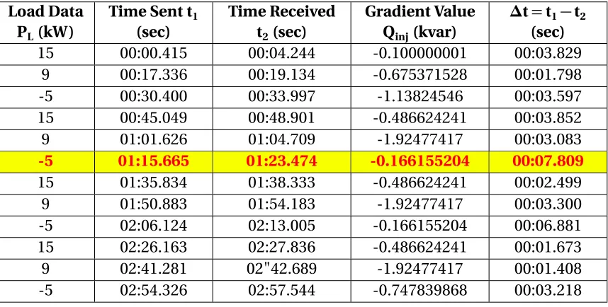
In communications, Round Trip Time (RTT) is the time taken for a signal to be sent plus
sent is Load data by the slaves and the acknowledgement received is the control command
Qs s t orQi n j. Table 3.1, 3.3 and 3.5 summarizes the RTT for each individual slaves as the
load changes. Slave-3 has the maximum RTT at 8.067 seconds and the average RTT for all
the slaves is around 3 seconds (Table 3.2, 3.4 & 3.6).
The GEH testbed is not completely exploited in this study. Some additional features that
could be tested using this testbed are: the transient behavior of the SSTs to the setpoint
update from the slaves, the effect of controller saturation, power limit of the SST on the
overall power loss reduction and voltage constraint & the lifetime of the controller subject
to multiple setpoint updates.
Table 3.1Round Trip Time for Slave-1
Load Data PL(kW)
Time Sent t1 (sec)
Time Received t2(sec)
Gradient Value Qinj(kvar)
∆t=t1−t2 (sec)
10 00:00.448 00:10.923 -0.100000001 00:10.475
5 00:21.394 00:25.793 -0.555991709 00:04.399
-3 00:36.529 00:41.631 -0.814027488 00:05.102
10 00:54.658 01:00.445 -0.345227122 00:05.787
5 01:10.758 01:15.278 -1.44209933 00:04.520
-3 01:26.000 01:30.138 -0.100000001 00:04.138
10 01:42.017 01:45.006 -0.345227122 00:02.989
5 01:58.112 01:59.848 -1.44209933 00:01.736
-3 02:10.832 02:15.688 -0.814027488 00:04.856
10 02:27.000 02:29.536 -0.100000001 00:02.536
5 02:42.371 02:44.411 -0.259374261 00:02.040
Figure 3.1Hardware setup of GEH Testbed
Table 3.2Metrics for Round Trip Time of Slave-1
Metrics
Table 3.3Round Trip Time for Slave-2
Load Data PL(kW)
Time Sent t1
(sec)
Time Received t2(sec)
Gradient Value Qinj(kvar)
∆t=t1−t2
(sec)
15 00:00.415 00:04.244 -0.100000001 00:03.829
9 00:17.336 00:19.134 -0.675371528 00:01.798
-5 00:30.400 00:33.997 -1.13824546 00:03.597
15 00:45.049 00:48.901 -0.486624241 00:03.852
9 01:01.626 01:04.709 -1.92477417 00:03.083
-5 01:15.665 01:23.474 -0.166155204 00:07.809
15 01:35.834 01:38.333 -0.486624241 00:02.499
9 01:50.883 01:54.183 -1.92477417 00:03.300
-5 02:06.124 02:13.005 -0.166155204 00:06.881
15 02:26.163 02:27.836 -0.486624241 00:01.673
9 02:41.281 02"42.689 -1.92477417 00:01.408
-5 02:54.326 02:57.544 -0.747839868 00:03.218
Table 3.4Metrics for Round Trip Time of Slave-2
Metrics
Table 3.5Round Trip Time for Slave-3
Load Data PL(kW)
Time Sent t1 (sec)
Time Received t2(sec)
Gradient Value Qinj(kvar)
∆t=t1−t2 (sec)
11 00:00.458 00:04.910 -0.675371528 00:04.452
7 00:15.444 00:19.750 -1.13824546 00:04.306
-8 00:31.517 00:34.609 -0.195416585 00:03.092
11 00:46.620 00:49.451 -0.349678576 00:02.831
7 01:02.713 01:05.000 -1.32400143 00:02.287
-8 01:15.791 01:20.151 -0.166155204 00:04.360
11 01:30.900 01:38.967 -0.349678576 00:08.067
7 01:51.041 01:53.802 -1.13824546 00:02.761
-8 02:05.097 02:08.653 -0.195416585 00:03.556
11 02:22.219 02:23.506 -0.349678576 00:01.287
7 02:37.283 02:38.352 -1.80373549 00:01.069
Table 3.6Metrics for Round Trip Time of Slave-3
Metrics
3.2
Large Scale System Simulation (LSSS) Testbed
One of the most important performance aspect of optimization algorithms in power system
is scalability. It is important to analyze the growth of computational and communication
complexity as the number of nodes in the system grows. These aspects not only enable the
realization of field implementation of such an algorithm but also play a major role in the
cost of implementation.
LSSS is a complete simulation platform that would test the performance of applications
developed in DGI framework on large systems with ease. The main difference between
the LSSS and GEH testbed is that the actual distribution system is simulated in LSSS
com-pared to the physical hardware in GEH. There are various potential distribution softwares
(Open source:OpenDSS, GridLabDand Proprietary:CYME, Milsoft) available in the market
that can simulate large distribution systems but they need to be interfaced with DGI. The
process of interfacing is not straight-forward and usually requires development of new
adapters that is not already present in the DGI framework. The advantage of using such a
software could be that the benchmark systems like IEEE 34 and IEEE 123 node systems are
readily available in these software platforms for testing. Many utilities have a simulation
model of their circuits in one of these softwares. As mentioned interfacing these softwares
with DGI becomes complicated. On the other hand, the VVO algorithm implemented being
a model-based approach already holds the model of the system. This model can be utilized
to simulate the system in DGI rather than using other distribution softwares.
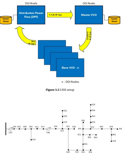
For simplicity and to still be able to model large systems in a simulation platform, a
performing power flow studies on this model as shown in Fig. 3.3. In the analysis of Large
systems the SSTs can be modelled or approximated as constant P & Q loads. The DPF block
(which models the distribution system) will send its current load data and Voltage Regulator
settings to master directly. The master will run the VVO application based on the current
state of system (when communication is ideal and there is no packet drops). The master
determines the optimal control settings which are then sent to the slaves. The slaves select
appropriate devices under its group in the DPF and sends the optimal settings which gets
updated in DPF. The state change in the system is assumed to occur every 5 minutes.
Modified versions of IEEE 34 node system and IEEE 123 node system are implemented
in the LSSS tested. The IEEE 34 node system is used to validate the testbed while various
performance metrics are analyzed using the IEEE 123 node system.
3.2.1
IEEE 34 Node System
The modified version of the standard IEEE 34 node system (named FREEDM 34 node
sys-tem) is as shown in Fig. 3.4. In this system, all traditional distribution transformers are
replaced by SSTs and all SSTs have both load and PV connected. There is no transformer
be-tween the node 832 and 888. In this system, a three-phase controlled LTC at the substation
and a VR are the only volt/var devices retained from the original 34 node system. All shunt capacitors are removed since SSTs can provide sufficient reactive power for the purpose of
VVC.
Figure 3.3LSSS setup
the DGI framework.
3.2.1.1 24-hour Simulation
To simulate the operation of the test feeder on a typical day, a 24-hour net load profile with
a 5-min resolution is utilized as shown in Fig. 3.6. The goal of this simulation is to validate
the results of the testbed against a non real-time implementation of the same system
pro-posed in[31]. For simplicity, the VR tap positions are assumed to be fixed at[8 8 8]and the LTC tap is fixed at1.05. All the DGI nodes runGroup Management→State Collection
→Volt VAR Optimizationin sequence. TheLoad Balancingmodule is excluded in this setup.
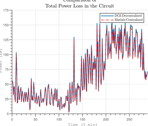
The data from the 24-hour DGI simulation is compared with the results of a centralized
implementation of same circuit under the same operating conditions in Matlab. The
24-hour maximum and minimum voltage throughout the circuit is shown in Fig. 3.7 and 3.8
respectively. Total loss in the system for the 24-hour period is shown in Fig. 3.9. It is observed
that the DGI data closely follow the Matlab results. Since there is no voltage regulation
modelled in the circuit, low voltage violation is observed during peak load conditions
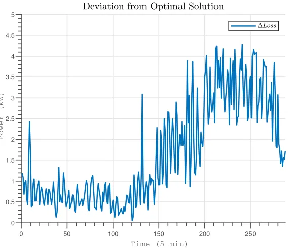
(Fig. 3.8). The overall power loss in the circuit is utilized to verify the optimality of the
decentralized algorithm (Fig. 3.9). Fig. 3.10 shows that the deviation of the decentralized
solution from the optimal centralized solution implemented in Matlab. The results indicate
that the maximum deviation throughout the 24-hour run is only4.2839kW as shown in
Fig. 3.10, which implies that the performance of Decentralized algorithm is very close to the
optimal solution. The deviation is observed due to the fact that the optimalQi n j commands
generated by the master is averaged at the slaves before being dispatched to the SSTs while
in the centralized implementation these commands are directly dispatched to the SSTs
Fig. 3.11 shows the overall delay in the DGI. Delay is calculated as the time taken for
the System to receive theQi n j e c t i o ncommands soon after the current load of the system
changes. It is observed that the maximum delay in the communication is around0.3973
secs which is very low compared to the 5 minute interval requirement for VVO. This is due
to the fact that the number of DGI nodes is very low for the 34 node system and VVO is
the only application running on all the DGI nodes. Hence, application latency as well as
communication latency is expected to be low. Since a Local Area Network was utilized to
test the setup, there was no data loss (packet drop) during the 24-hour simulation.
Figure 3.5Grouping of SSTs in FREEDM IEEE 34 Node System
3.2.2
IEEE 123 Node System
IEEE 123 node feeder is a system with a normal voltage of 4.16 kV, as shown in Fig. 3.12[30]. It is characterized by its many laterals and unbalance. A distribution transformer, between
nodes 61 to 610 steps down the voltage to 480V. There are four VRs in the circuit as marked
0 50 100 150 200 250
Time (5 min)
0% 20% 40% 60% 80% 100%
Load Multiplier
Figure 3.624 hr Load Profile for the FREEDM 34 Node system
0 50 100 150 200 250
Time (5 min)
0.95 0.96 0.97 0.98 0.99 1 1.01 1.02 1.03 1.04 1.05
Voltage (p.u.)
0 50 100 150 200 250
Time (5 min)
0.85 0.86 0.87 0.88 0.89 0.9 0.91 0.92 0.93 0.94 0.95 0.96 0.97 0.98 0.99 1 Voltage (p.u.)
Figure 3.8Minimum Voltage in the FREEDM 34 Node System
0 50 100 150 200 250
Time (5 min) 0 25 50 75 100 125 150 175 Power (kW)
0 50 100 150 200 250
Time (5 min) 0
0.5 1 1.5 2 2.5 3 3.5 4 4.5 5
Power (kW)
Figure 3.10Deviation from the Centralized Solution
0 10 20 30 40 50 60 70 80 90 100
Iteration Number 0.2
0.25 0.3 0.35 0.4
Time (secs)
With the switch settings as shown in Fig. 3.12, the circuit is a radial system with unbalanced
line segments and load. These VVC devices are needed to maintain an acceptable voltage
profile under all operating conditioins. The VRs have±16 tap position range with±10% of
maximum votlage change. The regulator VR1 is three-phase controlled while the other VRs
are single phase controlled. The IEEE 123 node system doesnot have any DRER by default.
Figure 3.12Simple Diagram of the IEEE 123 Test System
To implement a more practical smart distribution system, the following changes are applied
to the IEEE 123 node test feeder:
1. Loads are increased by 10% to create a more severe votlage drop.
3. All VRs are single phase controlled
4. All CAPs are removed, since the SSTs can provide sufficient reactive power for VVC.
Table 3.7Nodes with PV system in 123 Node Feeder
Node ID
Phase A 9, 48, 49, 52, 65, 76, 82, 109, 113 Phase B 22, 48, 49, 65, 76, 99
Phase C 6, 16, 48, 49, 65, 76, 92, 103
There are 15 PV nodes out of the 85 Load nodes in the system. The PV nodes are assumed
to be connected to the system through a SST while the Load nodes are assumed to be
connected to the system through a Distribution Transformer. Hence, there are 15 SSTs in
the circuit, indicated as green nodes in the Fig. 3.13. Based on the gradient, the SSTs with
approximately sameQc m d s were grouped as indicated using blue circles in the Fig. 3.13.
Af-ter grouping there are 12 DGI slaves in the circuit. The Voltage regulators require controllers
as well and these are modelled using DGI to facilitate communication between Master and
the controllers. Hence, in total there are 18 DGI nodes (1 DPF, 1 Master, 12 Slave & 4 VR
controllers). Each DGI node runsGroup Management→State Collection→Load
Balanc-ing→Volt VAR Optimizationin sequence. The Load Balancing application even though
applicable only in a microgrid environment, is still scheduled before the VVO application
Figure 3.13FREEDM 123 System with location of PV nodes and grouping of slaves
3.2.2.1 24-hour Simulation
To simulate the operation of the test feeder on a typical day, a 24-hour load profile & PV
profile with a 5-min resolution is utilized as shown in Fig. 3.14. The goal of this simulation
is to analyze the performance of the DGI under higher complexity of the system. By adding
the Voltage module along with VAR module in the VVO optimization algorithm and also
including Load Balancing algorithm at each time step the computation complexity is
in-creased profoundly. The number DGI nodes running distributedly is 18 in the 123 node
system which is much higher than the 8 DGI nodes in the 34 node case. (As it was observed
during the simulations that the complete control-update cycle is achieved within 1-min
0 50 100 150 200 250
Time (5 min)
0% 20% 40% 60% 80% 100%
Load (%)
Figure 3.1424 hr Load Profile for the FREEDM 123 Node system
The following plots show the 24-hour simulation results of FREEDM 123 node system which
are again compared with the results obtained from a similar setup running on Matlab:
1. Fig. 3.15 shows the plot of maximum voltage in the circuit. The maximum voltage
jumps from 1.0 p.u. to 1.025 p.u. at around 200 minutes due to the tap change in the
Voltage Regulators (Fig. 3.19 and 3.20). The maximum voltage in the circuit does not
violate the upper limit constraint of 1.05 p.u.
2. Fig. 3.16 shows the plot of minimum voltage in the circuit vs simulation time. The
minimum voltage is observed to constantly vary over the 24-hour run due to variation
in load and PV profile throughout the day. The voltage profile does not violate the
lower bound constraint of the optimization problem , i.e., 0.95 p.u.