POSTPROCESSING OF SASSI SOIL-STRUCTURE INTERACTION RESULTS FOR THE DESIGN OF CONCRETE NUCLEAR STRUCTURES
Carlos Coronado1, Neha Gidwani2, and Farhang Ostadan3
1Senior Engineer, Bechtel Power Corporation, Frederick, MD 2Senior Engineer, Bechtel Power Corporation, Frederick, MD
3Bechtel Fellow and Chief Soils Engineer, Bechtel National, San Francisco, CA
ABSTRACT
Most nuclear power plant (NPP) buildings are reinforced concrete (RC) panel or shell type structures. The seismic design of these structures is generally carried out using results from refined finite element models. For this purpose, seismic analyses are typically conducted using the computer program SASSI, which is currently the industry standard for the soil-structure interaction (SSI) analysis of NPP buildings. On the other hand, standard structural codes such as GTSTRUDL, SAP2000 or ANSYS are used for the static load analyses. As a consequence, two sets of independent results, seismic and static, must be parsed (imported) and combined, for the seismic design or evaluation of NPP structures. Such data parsing, processing and combination is typically done using in-house spreadsheets, databases and custom computer codes, which are limited in scope and lacking graphical data verification capabilities, thereby making the processing of seismic design data difficult to verify and prone to error.
This paper summarizes a new approach for the parsing, processing and visualization of seismic data for analysis and design of NPP structures. Static and dynamic analyses are carried out with the same finite element model, using ANSYS and SASSI computer programs, respectively. The method imports and maps the dynamic solution from SASSI into the ANSYS computer code in order to closely depict the dynamic solution graphically using acceleration and stress contour plots. After evaluation of the dynamic solution, static and dynamic results are combined using the appropriate set of load combinations for reinforced concrete design. In particular, demand to capacity ratios (DCR), for both element-based and section-cut design methods, are calculated and graphically reported for easy review and verification of the seismic design. A typical nuclear structure is analyzed and designed using the subject approach. Comparisons against traditional methods of analysis and design are provided, which show the benefits of the new methodology for verifying and streamlining the seismic analysis and design of NPP buildings.
INTRODUCTION
Most nuclear power plant (NPP) buildings are reinforced concrete (RC) panel or shell type structures. The seismic design of these structures is generally carried out using results from refined finite element models. For this purpose, seismic loads are typically calculated in the form of maximum nodal accelerations, maximum element forces, or time histories using the computer code SASSI. For static analysis, standard structural codes such as GTSTRUDL, SAP2000 or ANSYS are used. As a consequence, two sets of independent results, seismic and static, must be parsed (imported) and combined for the seismic design of NPP structures. These results are typically combined using one of the following three methods:
base shear obtained from direct dynamic analysis. Method A has been adopted as an acceptable method for stress analysis in the upcoming version of ASCE4 and is permitted to be used for design. The main advantage of this method is that the seismic and static structural models need not be the same. Therefore, a coarser FE model of the structure can be used for the SSI analysis.
Method B: In this method, peak/maximum element forces and moments from the SSI analysis are combined with corresponding static analysis results. These peak forces and moments can be used directly or averaged over certain length to get section-cut forces for combination with static results. Method B results in much more realistic demand forces compared to method A; but, the same FE model must be used for the seismic SSI and static analyses of the structure. It must be noted that, until very recently, limitations in computer capacity and the program SASSI did not permit the use of the detailed finite element models developed for the static analysis for performing the seismic SSI analysis. This issue has been resolved in the new version of SASSI (SASSI2010), which has permitted to improve the methodology for developing seismic design loads.
Method C: In this method, time histories of element forces and moments or section-cut results from the SSI analysis are combined with results from the static analysis. Similar to method B, the same FE model must be used for the SSI and static analyses of the structure. Method C accounts for the actual timing of the element forces i.e., it does not assume that maximum seismic forces occur at the same time for all the elements, as implied in Method B. However, for stiff shear wall type structures that are typically used for NPP structures, the benefit of Method C compared to method B is very limited.
The data parsing, processing and combination of results required by above methods is typically done using in-house spreadsheets, databases and custom computer codes, which are limited in scope and lacking graphical data verification capabilities, thereby making the processing of seismic data difficult to verify and prone to error. The shortcomings of the current state of practice have been pointed out by NIST (2011) report, which states that: “no guidelines are generally available on how to process and interpret the post-processing of finite element output (i.e. averaging, smoothing, neglecting, etc…) for NPP structures”.
Graphical post-processing of finite element results using contour and vector plots have been the standard in commercial finite element codes since the early 80s. Currently available finite element post-processors are highly mature and can be used to visualize and manipulate a variety of finite element results. In this paper, the authors propose the use of ANSYS post-processor (POST1) for the parsing, processing and visualization of SASSI seismic results. ANSYS is a highly user friendly program, which can be easily customized to meet the user’s needs. This code is widely used in the nuclear industry to conduct static, dynamic, thermal and fluid structure interaction analyses of NPP structures. Therefore, the use of ANSYS for post-processing SASSI results brings a unified visualization environment for seismic and static analyses results and an integrated approach for analysis and design of NPP structures.
structure is analyzed and designed using combination Method B. Comparisons against traditional methods of analysis and design are provided, which show the benefits of the proposed methodology for verifying and streamlining the seismic analysis and design of NPP buildings.
POSTPROCESSING OF PEAK NODAL ACCELERATIONS
Before discussing the advantages of the combined SASSI/ANSYS analysis for stress analysis and design, the advantages of importing SASSI results into ANSYS in terms of maximum acceleration (Method A) are presented. SASSI reports the acceleration response (ax, ay, az) of each node i of the
structure due to each component of the design ground motion (X, Y, Z). Table 1shows the typical format of the acceleration output file. The maximum acceleration response of node i in a particular response direction (i.e., , or ) is calculated by combining the nodal accelerations due to each of the
three spatial components (X, Y, Z) of the design earthquake, as detailed in RG 1.92. Thus for each node, the 100-40-40 or SRSS combination rules are typically used as detailed in Table 2. For instance,
| | | | | |; where |aixx|>|aixy|>|aixz| are the acceleration responses in the x direction
respectively due to the X, Y and Z components of the earthquake.
Table 1: Sample SASSI output: peak absolute acceleration response due to ground motion component X
N.P.1 X-ACC2 AT TIME3 Y-ACC4 AT TIME5 Z-ACC6 AT TIME7 1182 0.265 10.250 0.001 10.290 0.002 9.090 1183 0.265 10.250 0.001 10.290 0.002 9.090 1185 0.265 10.250 0.001 10.290 0.002 9.090 1188 0.265 10.250 0.001 10.290 0.002 9.090
1Label of node i;2,4,6 x, y and z components of the acceleration response of node i due to ground
motion component X (i.e., aixx, aixy, aixz); 3,5,7 respectively time of peak responses aixx, aixyand aixz.
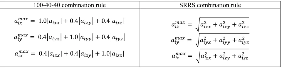
Table 2: Combination of peak absolute acceleration response 100-40-40 combination rule SRRS combination rule
| | | | | |
|
| | | | |
|
| | | | |
√
√
√
Figure 1: Typical maximum acceleration bubble plot
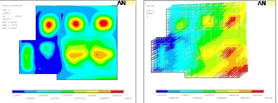
In this paper, it is demonstrated that contour plots are a better alternative for the presentation of maximum seismic acceleration response data. Contour plots are the standard for visualization of finite element results and can be used to display the acceleration response of the complete structure or a section of interest, as shown in Figures 2 and 3. The creation of these plots can be easily automated in ANSYS, which reduces the possibility of human error. For this purpose, SASSI acceleration data is read into ANSYS vectors (one for each acceleration component) and mapped to the nodes of the ANSYS finite element model for post-processing and further manipulation, if required. Figure 2 shows the maximum acceleration data previously depicted in Figure 1. As can be seen, the interpretation of results is easier using this type of representation. Additionally, seismic acceleration data can be presented using vector plots as shown in Figure 2, which provide information regarding the directionality of the seismic response of the structure.
Once acceleration data has been imported and mapped into ANSYS nodes, the creation of pseudo-static seismic loads is straightforward. It only requires the definition of point loads at each node, which can be calculated by multiplication of the acceleration vector by the mass matrix of the structure, which can easily be done using ANSYS parametric design language (APDL).
Figure 2: Maximum acceleration contour and vector plots for a typical building slab created in ANSYS using imported SASSI data
190 210 230 250 270 290
360 380 400 420 440 460 480 500
Y C
oordi
nat
e
(ft
)
X Coordinate (ft)
Maximum Accelerations (g) Diesel Generator Building - EL 677.25 ft Z 100-40-40 (Hard Rock - RG Ground Motion)
Maximum = 0.286g Average = 0.169g
1
MN
MX
.10872 .128407
.148093 .16778
.187467 .207153
.22684 .246527
.266213 .2859 NODAL SOLUTION
SUB =1 TIME=1 UZ (AVG) RSYS=0 DMX =.52181 SMN =.10872 SMX =.2859
1
.337747 .358199
.37865 .399102
.419553 .440004
.460456 .480907
.501359 .52181 VECTOR
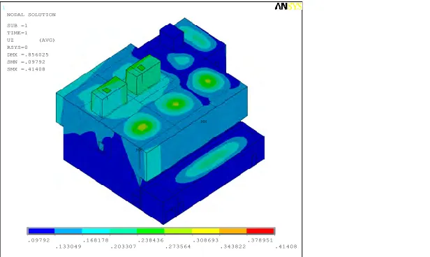
Figure 3: Maximum acceleration contour plot for the whole building created in ANSYS using imported SASSI data
From the above figures, it can be seen that one of the main advantages of graphic visualization of maximum acceleration is in the ability to quickly identify the areas of high acceleration in the entire structure, which empowers the design engineer to make requisite design modifications to improve the overall behavior of the structure. This would not be possible without the ability to visualize the dynamic responses zone by zone in the entire structure.
POSTPROCESSING STRESS RESULTS
Output from finite element codes used in nuclear applications (e.g., SASSI and ANSYS) is given in the form of element stresses, stress resultants, and/or internal element nodal reaction forces. Element stresses and stress resultants are normally given in the element coordinate system, while internal element reaction forces are in the global coordinate system. In many situations the seismic results and static results are in different coordinates systems, and stress/force transformations are required before their combination or visualization (e.g., to align the stress results with the main reinforcement directions). The steps required for this purpose are discussed in the section below. However, due to space limitations, the following discussion is restricted to post-processing of thick shell element results for combination with static results per Method B, described before. It must be noted that most NPP structures are modeled
using thick shell elements; therefore the following discussion is most relevant.
Shell/Plate Element Stress Results
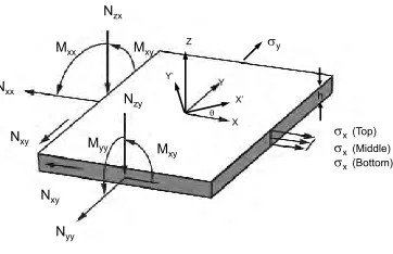
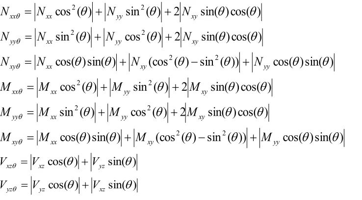
Shell element stress results (i.e., xx, yy, xy, xz and yz) are normally reported in the element coordinate system e.g., the Cartesian coordinate system XYZ shown in Figure 4
;
where the sign convention for these stresses should be consulted in the user’s manual of the computer code being used. In general, shell element stresses follow tensor notation and are transformed using the same rules. Shell element stress resultants per unit length (Nxx, Nyy, Nxy,Mxx, Myy, Mxy, Vzx, and Vzy), are shown in Figure 4,and are derived from element stresses. In general, the stress resultants are of most interest to the designer because they can be used to calculate the shell reinforcement using methods such as Wood-Armer (Park and Gamble, 1980), Sandwich model (Marti 1990) and others (Blaauwendraad 2010). Therefore, the following discussion concentrates on the post-processing of SASSI seismic stress resultants from the thick plate element in SASSI2010 and its combination with corresponding ANSYS static stress resultants.
1
MN
MX
.09792 .133049
.168178 .203307
.238436 .273564
.308693 .343822
.378951 .41408 NODAL SOLUTION
Figure 4: Shell Element Stress Resultants
As already mentioned, SASSI seismic results and ANSYS static results are typically reported in different coordinates systems. Shell stress resultants, Figure 4, reported in a particular coordinate system
XY can be transformed to an arbitrary set of axes X’Y’ —also shown in Figure 4— according to the tensor transformation rule, which is given by Equation (1), where is the angle between x’ and x. However, special considerations are required for transforming SASSI stress resultants, as described in the following section.
)
cos(
)
sin(
2
)
(
sin
)
(
cos
2
2
xx yy xy
xx
N
N
N
N
)
cos(
)
sin(
2
)
(
cos
)
(
sin
2
2
xx yy xy
yy
N
N
N
N
cos(
)
sin(
)
(cos
2(
)
sin
2(
))
yy
xx
xy
xy
N
N
N
N
)
cos(
)
sin(
2
)
(
sin
)
(
cos
2
2
xx yy xy
xx
M
M
M
M
)
cos(
)
sin(
2
)
(
cos
)
(
sin
2
2
xx yy xy
yy
M
M
M
M
cos(
)
sin(
)
(cos
2(
)
sin
2(
))
yy
xx
xy
xy
M
M
M
M
) sin( )
cos(
xz yz
xz V V
V
) sin( )
cos(
yz xz
yz V V
V
(1)
Transformation of SASSI stress resultants
SASSI generates output files of peak element resultants per unit length (i.e., Nxx, Nyy, Nxy, Mxx,
Myy, Mxy, Vzx, and Vzy ) for each earthquake direction (i.e., X, Y, and Z) and soil case used in the seismic
analysis (e.g., LB, BE and UB)1. Such resultants are provided in local coordinates at the integration points
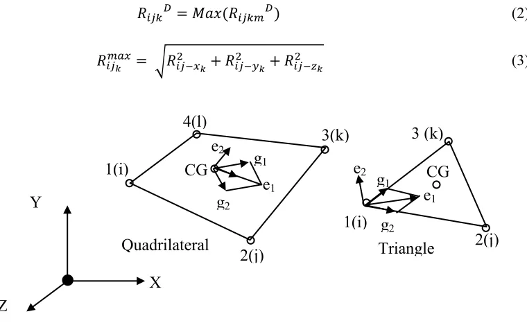
of each element (i.e., 1, 2, 3 and 4) and at the element centroid (CG), as shown in Table 3 and Figure 5.
Table 3: Sample SASSI stress resultants (kip, feet) for BE soil profile and Regulatory Guide 1.60 (RG 1.60) ground motion component Y
ID Node X Y Z Nxx Nyy Nxy Mxx Myy Mxy Vzx Vzy
1 1 -116.1 -0.5 37.2 -9.1 7.0 -3.7 -14.4 0.8 -2.8 -2.8 3.7 1 2 -116.1 -0.5 39.3 -9.5 2.4 5.0 -14.5 0.3 -3.7 -2.8 3.0 1 3 -114.2 -0.5 39.3 -3.8 1.3 -5.6 -16.5 0.5 -4.0 -2.2 3.0 1 4 -114.2 -0.5 37.2 -3.5 5.9 -4.3 -16.4 -0.6 -3.1 -2.2 3.7
1
Lower bound (LB), best estimate (BE) and upper bound (UB) soil profiles.
yX
x (Top)
x (Bottom)
x (Middle)
Nzx
Nxx
Nyy
Nxy
Nxy Myy
Mxx Mxy
Mxy
Nzy h
Y Z
Y’
To reduce the element data, for each motion component, the stress resultants for element i can be conservatively calculated as the maximum of the stress resultants reported at the gauss points and element CG, as shown in Equation (2), where i = element number, R = N, M or V, j = xx, yy, xy, zx or zy, k = LB, BE or UB, m = 1, 2, 3, 4 or CG, and D is the ground motion direction X, Y or Z. The data reduction also simplifies the combination with ANSYS results, which only reports results at the element CG. After reducing SASSI data, the maximum stress resultants, for each design motion and soil profile, are calculated herein using the SRSS combination rule, as defined in RG 1.92. In particular, the maximum stress resultant for each ground motion under consideration is calculated per Equation (3); where R, i, j
and k are previously defined.
(2)
√ (3)
Figure 5: SASSI local axes e1 and e2 and nodal nomenclatures
Note that maximum element resultants calculated per Equation (3) occur at different times. Nevertheless—for design purposes—the seismic demand is conservatively maximized, in combination Method B, by considering that the maximum stress resultants occur at the same time. For reinforced concrete design, seismic safe shutdown earthquake (SSE) and static demands are combined per ACI 349-06 ultimate load combination 9-9; see Equation (4), where it must be noted that the SSE demand for shell elements (Ess) results in 28 = 256 load cases due to the sign permutations required to address seismic load
reversals, as summarized in Equation (5).
(4)
±Nxx ±Nyy ±Nxy ±Mxx ±Myy ±Mxy ±Vzx ±Vzy (5)
These 256 permutations must be applied before performing the stress transformations given by Equation (1), which increases the computational cost given the multiple soil profiles and ground motions used for the design of NPP structures. However, the number of stress transformations and sign permutations can be significantly reduced by maximizing Equation (1) and observing that current ACI 349-06 practice does not require considering the simultaneous interaction/action of the eight (8) shell stress resultants given by Equation (5), since they have different phases. In particular, only Moment and Axial force (i.e., ±Nxx and ±Mxx or ±Nyy and ±Myy), and Shear and Axial force interaction (i.e., ±Nxx and
3 (k)
1(i)
2(j)
Triangle
e
1e
2Quadrilateral
2(j)
1(i)
4(l)
3(k)
(k)
CG
e
1e
2CG
X
Z
Y
g
2g
1±Nxy, ±Nyy and ±Nxy, ±Nxx and ±Vzx, ±Nyy and ±Vzy), need to be considered for design of reinforced concrete
walls and slabs.
Taking into account the above discussion, stress transformations given by Equation (1) are maximized here using Equation (6), which envelopes the results obtained after applying the 256 permutations of Equation (5) followed by Equation (1). In other words, only one stress transformation operation is required by using Equation (6), compared to the 256 operations required by Equations (5) and (1), which is a significant computational saving. Therefore, in this paper, SASSI stress resultants for Method B are post-processed using Equation (6).
)
cos(
)
sin(
2
)
(
sin
)
(
cos
2
2
xx yy xy
xx
N
N
N
N
)
cos(
)
sin(
2
)
(
cos
)
(
sin
2
2
xx yy xy
yy
N
N
N
N
)
sin(
)
cos(
))
(
sin
)
(
(cos
)
sin(
)
cos(
2
2
xx xy yy
xy
N
N
N
N
)
cos(
)
sin(
2
)
(
sin
)
(
cos
2
2
xx yy xy
xx
M
M
M
M
)
cos(
)
sin(
2
)
(
cos
)
(
sin
2
2
xx yy xy
yy
M
M
M
M
)
sin(
)
cos(
))
(
sin
)
(
(cos
)
sin(
)
cos(
2
2
xx xy yy
xy
M
M
M
M
) sin( )
cos(
xz yz
xz V V
V
) sin( )
cos(
yz xz
yz V V
V
(6)
Referring to a particular shell element i, the post-processing of peak seismic stress resultants reported by SASSI—for each ground motion (e.g., WUS, CEUS, RG)2 and soil profile (e.g., LB, BE,
UP)—can be summarized in the following steps, applicable to combination Method B:
1. Use Equation (2) for calculating one set of seismic stress resultants, at the element CG, for each ground motion direction (X, Y, Z).
2. Use Equation (3) to calculate the maximum seismic stress resultants in the element local coordinate system (XY).
3. Use Equation (6) to transform the maximum seismic stress resultants to match the main reinforcement directions, referred to as X’ and Y’ directions.
4. Use Equation (1) to transform the static stress resultants to match the main reinforcement directions, referred to as X’ and Y’ directions.
5. Use equation (4) to combine seismic and static element resultants; where appropriate sign permutations must be used for the maximum seismic forces, to account for load reversals, as described in the following section.
Above steps are easily implemented using ANSYS APDL scripts. Sample results are shown in Figure 6, which shows typical SASSI stress resultants after transformation and combination with ANSYS static results.
Figure 6: Sample stress resultants contour plots
POSTPROCESSING OF DESIGN RESULTS
This section presents the overall procedure for calculating and presenting demand to capacity ratios (DCR) of critical walls and slabs to meet ACI 349 using load combination Method B. For the sake of brevity, DCR are calculated, in an element by element basis and only for moment and axial force interaction. However, it must the noted that a complete design also requires in-plane shear, shear friction and out-of-plane shear checks. In particular, the following steps are required for evaluating the walls, slab and base mat subjected to moments and axial forces per ACI 349.
1. Calculate the interaction diagrams for the X’ and Y’ reinforcement directions shown in Figure 7. 2. Determine the design moment and normal (membrane) force resultants acting at the centroid of each
element, using the procedures described in the previous section. In particular, the factored design moment (Mu) can be calculated by combining the bending and twisting moment resultants per
Equations (7) and (8)3, which are a conservative simplification of those reported by Park and Gamble
(1980). Similarly the membrane forces are calculated per Equations (9) and (10), where the sign of the seismic membrane forces (i.e., , ) must be permuted to account for seismic load reversals;
refer to Figure 7 for further details.
3E = Earthquake or seismic demand, S = static demand
N
xxθN
yyθ3. Verify the appropriate maximum reinforcement limit.
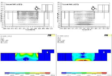
4. Verify that the demand to capacity ratio (DCR) at each wall/slab location (i.e., centroid of each shell element part of the wall) for each load combination is less than 1.0. This is done by plotting the results in ANSYS as shown in Figure 8
,
which also compares the DCR bubble plots vs. DCR contour plots. As can be seen, the contour plots are easier to read and interpret.Mux = (| | + | |) + (| | + | |) (7)
Muy = (| | + | |) + (| | + | |) (8)
Pux= ± + (9)
Puy= ± + (10)
Figure 7: Interaction of Normal force and Out-of-Plane Bending
CONCLUSION
With the advent of the new version of SASSI (SASSI2010) and access to high capacity desktop computers, the same detailed finite element model typically used in static analysis can be used for seismic SSI analysis. This development provides a new opportunity for design of concrete members for NPP structures. The graphical design process presented in this paper includes parsing, processing and visualization of seismic data in combination with static results for design. A typical example of a nuclear structure analyzed and designed using the computer programs, ANSYS and SASSI, is utilized to demonstrate the new design approach. In this method, the dynamic loads are imported and mapped into the ANSYS model in order to closely depict the dynamic solution graphically using acceleration and stress contour plots. Visual observation of the dynamic solution for the entire structure is proved to be very effective to improve the design in areas that show significant amplification of motion. After evaluation of the dynamic solution, static and dynamic results are combined using the appropriate set of load combinations for reinforced concrete design. In particular, maximum seismic accelerations and demand to capacity ratios (DCR) are calculated and graphically reported for easy review and verification of the seismic analysis and design. In addition, this paper demonstrates that the proposed methodology allows for easy and streamlined verification compared with traditional methods for the seismic analysis and design of NPP buildings.
REFERENCES
American Society of Civil Engineers (2000). Seismic analysis of safety-related nuclear structures and commentary. Reston, VA.
Computers & Structures, Inc. (2000). “SAP2000, Integrated Software for Structural Analysis & Design,” Version 10.0.1, Berkeley, CA.
Ostadan, F. and Deng, N. (2011). “Bechtel version of SASSI2010 – A System for Analysis of Soil-Structure Interaction,” Version 1.1, Geotechnical and Hydraulic Engineering Services, Bechtel National Inc., San Francisco, CA.
ANSYS. (2010). ANSYS Mechanical APDL Structural Analysis Guide, Release 13.0, ANSYS, Inc., Canonsburg, PA.
ACI COMMITTEE 349. (2006). Code Requirements for Nuclear Safety-Related Concrete Structures: (ACI 349-06) and Commentary, an ACI standard. Farmington Hills, Mich, American Concrete Institute.
NIST. (2011). “Concrete Codes and Standards for Nuclear Power Plants: Recommendations for Future Development,” Nuclear Energy Standards Coordination Collaborative (NESCC), National Institute of Standards and Technology, Gaithersburg, USA.
Blaauwendraad, J. (2010). Plates and FEM surprises and pitfalls. Dordrecht, Springer.
http://site.ebrary.com/id/10361872.
Marti, P. (1990). Design of concrete slabs for transverse shear. ACI Structural Journal, 87(2). Park, R., & Gamble, W. L. (1980). Reinforced concrete slabs. New York, Wiley.
U.S. Nuclear Regulatory Commission (2006). Regulatory Guide 1.92, “Combining Modal Responses and Spatial Components in Seismic Response Analysis”