Design and Implementation of Novel Energy Efficient Gaussian Filter

Design and Implementation of Novel Energy

Efficient Gaussian Filter

Shalini Upadhyaya1, Shweta Agrawal2

Research scholar, Dept. of Electronics and Communication, SRCEM Banmore, Morena, India1 Assistant Professor, Dept. of Electronics and Communication, SRCEM Banmore, Morena, India2

ABSTRACT: Most of the modern portable devices exhibits multimedia applications and demand energy efficient designs. The Gaussian filter is commonly used to remove noise while maintains the structure of the object in the scene. In this paper, a novel reconfigurable Gaussian smoothing filter (R-GSF) architecture is proposed. The proposed filter can be reconfigured to provide higher energy saving at the cost of small loss of quality. The effectiveness of the proposed filter is evaluated and compared over the existing filters. Simulation result shows proposed filter requires 13%, reduced area over existing energy scalable Gaussian smoothing filter. Further, the proposed filter reduces 57.2% delay over the existing. Finally, the proposed R-GSF filter requires 53.2% reduced energy consumption over the existing filter.

KEYWORDS: Digital Signal Processing (DSP), Gaussian Filter, Image Processing, Integrated Circuits, VLSI, Low Power Design.

I. INTRODUCTION

In the modern VLSI design for the portable gadgets, the prime concern is the power and performance. As the portable devices are operated with a limited power source, large power consumption causes rapid discharge of battery. Therefore, energy efficient design is challenging task and become severe for the portable device because it requires large battery size and requires costly cooling circuitry to maintain the temperature of the device.

The modern portable devices frequently employ multimedia applications that produce output for human consumption [1]. Due to the limited visual perception, human can accept errors. Moreover, the noise in the present electronic devices can come from anywhere e.g. while transmission, storage etc. In order to remove the effect of the error, filter is required. Most commonly employed filter in image processing is the smoothing filter. Different algorithms are developed in the literature to efficiently filter the noisy input image [2], [3]. The concept of coefficient approximation into power of two is presented such that resulting coefficients can be realized without any multiplication logic. Other approach utilizes the similarity existing in the neighbouring pixels [4].

In contrast to different algorithms, different architectural approach where computation sharing is done is also demonstrated. In addition to these design, an energy scalable Gaussian smoothing filter (ES-GSF) [5] is also presented which provides trade-off between quality and energy. The ES-GSF is based on the principle of consideration of varying size coefficient with respect to the central coefficient. The existing architectures still having higher complexity and must be reduced to fit the design within the modern portable devices.

II. APPROXIMATE GSF ARCHITECTURES

The mathematical model of the Gaussian distribution can be represented by the Eq. 1 given below.

( ) = 1 √2

( )

(1)

Where, m, g andσrepresent the mean or average, gray level and the standard deviation of the noise respectively. As the Gaussian smoothing is commonly employed in different image processing applications such as edge detection [2] to remove unwanted edge, image mosaicing and tone mapping etc., it requires two dimensional (2D) Gaussian expression due to the 2D nature of the image. The 2D Gaussian expression is represented by Eq. 2.

( , ) = ( ) (2) Where, x and y are the variables representing the coordinate while sigma representing the standard deviation.

The processing of image through the above expression requires implementation of above expression in the software form which performance inefficient. Therefore, hardware efficient implementation is done for the GSF. From VLSI design point of view, direct implementation of the above expression is area and performance efficient. Therefore, the above expression can be approximated by a matrix called kernel. The image processed through the Gaussian kernel provides the same result as the above expression. The accurate representation of the Gaussian expression using Gaussian kernel of 5x5 size is given by eq. (3).

⎣ ⎢ ⎢ ⎢

⎡0.0030_0.0133 0.0133 0.0219 0.0133 0.0030 0.0219 0.0133 0.596 0.0983 0.596 0.0983 0.1621 0.0983 0.0996 0.0983 0.0996 0.0133 0.0219 0.0133 0.0030 0.0133 0.0219 0.0133 0.0030⎦

⎥ ⎥ ⎥ ⎤

(3)

This matrix is achieved by varying the value of variable x, y from -2 to +2 with σ=1. From the Figure it can be seen that direct implementation requires floating point multiplier to achieve smoothened pixel, therefore different approximations are done to achieve kernel coefficient which are hardware efficient. Based on the approximated coefficients, different architectures are developed. Following subsection details different algorithms and architectures developed for the energy efficient smoothing.

2.1 Fixed-point Gaussian Kernel

A fixed point implementation of Gaussian coefficient is used to achieve approximate kernel [6]. In fixed point representation in (l, m) format, l represents the number of bits while m represents location of coefficient least significant bits. Fig. 1 shows the Gaussian smoothing kernel rounded to the (2, -4) and (6, -8) data formats.

1 2 ⎣ ⎢ ⎢ ⎢

⎡0₀ 0 0 0 0 0 0 1 2 1 2 3 2 1 2 1 0 0 0 0 0 0 0 0⎦⎥

⎥ ⎥ ⎤ 1 2 ⎣ ⎢ ⎢ ⎢

⎡1₃ 3 6 3 1 6 3 15 25 15 25 41 25 15 25 15 3 6 3 1 3 6 3 1⎦⎥

⎥ ⎥ ⎤

(a) (b)

Fig. 1: GSF kernel data format a) (2, -4) b) (6, -8).

These kernels reduce implementation complexity of the Gaussian filter which results in significant reduction in power, area and delay metrics at the same time the proposed kernels provide the acceptable output quality.

2.2 Approximate Parameterizable 2D GSF

The computation complexity of the floating point multiplier is very high which makes the direct implementation of the 2D Gaussian smoothing kernel energy inefficient. A digital approximation of the kernel coefficient presented in [7] that significantly reduces the implementation complexity of the Gaussian kernel. In this approximate kernel each coefficient is approximated in sum of power-of-two. As multiplication of any term with a constant having value in power of two will not require any hardware for implementation. The proposed Gaussian kernel with value in power-of-two is given by eq. 4.

⎣ ⎢ ⎢ ⎢

⎡ 0 2 2 +2 2 0

2 2 +2

2

2 +2 2 +2 2 +2

2 +2 2 +2 2 +2

2 +2 2 +2 2 +2

2 2 +2

2

0 2 2 +2 2 0 ⎦⎥

⎥ ⎥ ⎤

(4)

A simplified architecture is developed that utilized the kernel coefficients in the power-of-two form and compute the smoothened pixel. The architecture is shown in Fig. 2.

Fig. 2: Parameterizable 2D-GSF architecture.

2.3 SPAA-Aware 2D Gaussian Smoothing Filter

The existing smoothing filter exhibits high complexity which limits the energy-efficiency that can be improved by exploiting the property of image. A speed, power area and accuracy (SPAA) aware 2D Gaussian smoothing filter is demonstrated in [8] that exploits the neighbour pixel similarity existing within an image. This architecture significantly reduces the implementation complexity and exhibits significantly improved design metrics. The following subsection reveals the basic principle to reduce the complexity and architectural approach considered.

2.3.1 Neighbour Pixel Similarity (NPS)

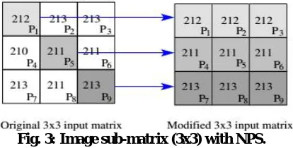
The adjacent pixels exhibit higher correlation in an image. This higher correlation in the image is due to the fact that image have smoothened nature and the large difference will occur only on the edge. As the natural and most of the images have edge which is very small in number, it makes assumption of adjacent pixel to be nearly same true. In case of image smoothing, an image sub-matrix is considered for processing for example a 5x5 or 3x3 image sub-matrix. Therefore, concept of neighbour pixel to be same significantly reduces the computation complexity of the smoothening filter. For example, an original sub-matrix of size 3x3 as shown in Fig. 3 is replaces all pixels of a row by its single value. This replacement will not cause large error the values are very near.

Fig. 3: Image sub-matrix (3x3) with NPS.

Fig. 4: Approximate-GSF on 3x3 image submatrix.

The procedure is shown in Fig. 4 where pixels of each row is approximate by its diagonal pixel value and the row coefficient of the kernel are added to achieve the desired multiplier. This constant multiplier is then multiplier with the approximated pixel to achieve the smoothened pixel. From the figure can be observed that it requires only five multipliers with few adders to added the coefficients.

III. ENERGY SCALABLE GAUSSIAN SMOOTHING FILTER (ES-GSF) ARCHITECTURE

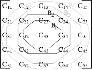
The modern devices demand reconfigurable architecture due to the ever changing requirement of the real-time applications. Based on the applications and its criticalness, the design should be able to adapt different energy-quality trade-off which is achieve by the energy scalable GSF architecture [9]. This architecture exploits the concept of significant/non-significant coefficients and presented significant and non-significant boundaries as shown in Fig. 5.

Fig. 5: Kernel coefficient with boundaries.

It observed that value of coefficient decrease from centre to the boundaries therefore, boundary B1 is more

significant (due to having more weight) over the B4. The ES-GSF exploits the non-significant boundaries to achieve

desired quality energy trade-off. Further, the coefficient of the given boundary is of same value, the resulting architecture will compute sum of all pixel of that boundary and multiplied with the coefficient.

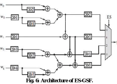
Fig. 6: Architecture of ES-GSF.

It can be observed that energy scalable GSF architecture computes value of different boundaries which are getting adder with the significant boundaries. For example, W0 and W1 both providing smoothing pixel via only boundary B1.

Another boundary B2 is added with this to generate smoothened pixel of higher quality at the cost of increased

complexity. In the similar way non-significant boundaries are added with the significant to improve the quality at the cost of computational complexity. Therefore, ES-GSF provides trade-off between performance and quality.

IV. EXPERIMENTAL RESULT & ANALYSIS

The efficacy of the proposed filter is evaluated over the existing architectures by implementing designs on MATLAB and Tanner computing the quality metrics [10], [11] and design metrics by simulating with benchmark [12], [13] inputs as shown in Fig. 7. On the other hand, to evaluate the design metrics designs are implemented on Tanner schematic editor. Finally, the design metrics such as area, power and delay are extracted for the proposed and existing designs and compared.

Fig. 7: Lena image for benchmark input. 4.1 Quality and Design Metrics

Various quality and design parameters are used to evaluate the design. This subsection introduces the different quality parameters which are used in our design.

4.1.1 Mean Square Error (MSE)

The MSE for an input image I and noisy output image K, is defined by the expression given below.

= ∑ ∑ [ ( , )− ( , )] (5) Where, variables m and n represent the number of row and column of the image.

4.1.2 Mean Error Distance (MED)

4.1.3 Normalized Error Distance (NED)

NED is the mean error distance divided by the maximum value of original signal. Value of NED is independent of the size of the design and depends only of the kind of architecture. Therefore, NED quantify the error metrics of the technique better than the MED.

4.1.4 Peak Signal to Noise Ratio (PSNR)

The peak-signal-to-noise-ratio is the parameter used widely in image/video processing applications to quantify the amount of the noise present in the image and it is equal to the maximum signal power to the noise power. The mathematical expression that computes the PSNR in decibel is given by the equation below.

= 10. log ( ) (6) Where, SigI reflects the maximum signal value which for an image is 255.

4.1.5 Structural Similarity (SSIM)

The existing quality metrics signifies the quantity of error in the given input signal. In an image, the noise may be perceivable or it may not. If the noise is not perceivable noise will not affect the quality of the image. In order to compute the quality of the image i.e. perceivable errors present in the image a new quality metrics based on structural similarity (SSIM) is used. This quality metrics is becoming more popular in recent years.

Although, the SSIM better quantify the quality of the image, the more commonly used parameter is the PSNR.

4.2 Simulation results on MATLAB

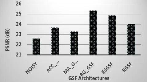
To evaluate the quality metrics of the proposed Gaussian filter, the proposed and existing filter architectures are implemented on the MATLAB and simulated with benchmark input image. Mean error distance, normalized error distance, PSNR and SSIM are computed for each Gaussian filter as shown in Table 5.1.

Table 5.1: Error metrics of different GSF.

Parameter MED MSE NED PSNR SSIM

Noisy 14.21 316.21 0.1755 22.59 0.7822

Acc_GSF 13.032 273.02 0.1484 23.66 0.8715

MA_GSF 13.61 297.82 0.1478 23.28 0.8579

BG_GSF 14.59 348.99 0.1373 25.34 0.9565

ESGSF 11.49 207.04 0.1507 24.85 0.9509

RGSF 10.77 185.36 0.1507 24.02 0.9034

It can be observed from the Table 5.1 that proposed R-GSF provides good quality over MA-GSF as shown in Fig. 8.

Fig. 8: PSNR for different GSF architectures

21 22 23 24 25 26

P

SN

R

(d

B

)

Similarly, Fig. 8 shows SSIM for different GSF architectures where proposed R-GSF provides higher SSIM over MA-GSF while provides little smaller SSIM over ES-GSF and BG-GSF architectures.

Fig. 9: SSIM for different GSF architectures

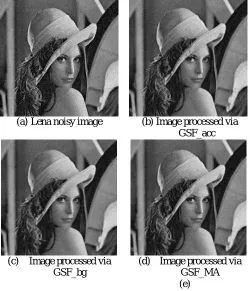
Finally, the processed image using different Gaussian filters as shown in Fig. 10 reflect that proposed GSF provides image of acceptable quality.

(a)Lena noisy image (b)Image processed via GSF_acc

(c) Image processed via GSF_bg

(d) Image processed via GSF_MA (e)

0.7822

0.8715 0.8579

0.9565 0.9509

0.9034

NOISY ACC_GSF MA_GSF BG_GSF ESGSF RGSF

(f) Image processed via ES-GSF

(g)Image processed via R-GSF

Fig. 10: Lena image filter via different GSF filters.

4.3 Design metrics comparison

The design metrics all GSF are computed by implementing on Tanner v14.1. The schematic of the proposed R-GSF is shown in Fig. 11. Similarly, other GSFs are also implemented on Tanner.

Fig. 11: Implementation of R-GSF on Tanner.

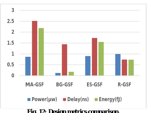
The spice netlist is generated from the schematics implemented on Tanner. The design metrics such are area, power and delay are extracted for each design and are compared to evaluate the effectiveness of proposed architecture over the existing. The area, power, delay and energy metrics for the different GSF architectures are shown in Table 5.2.

Table 5.2: Design metrics for different GSF.

Design

Area (#Tran)

Power (µw)

Delay (ns)

Energy (fJ)

MA-GSF 5264 0.8688 2.52 2.189

BG-GSF 1288 0.12144 1.446 0.175

ES-GSF 5812 0.901 1.73 1.55

R-GSF 5056 0.99 0.74 0.732

GSF is smaller over all GSF architectures. Finally, the energy efficiency of the BG-GSF is high over the all the existing GSFs as shown in Fig. 12.

Fig. 12: Design metrics comparison.

Fig. 13 illustrates the area requirement by the different GSF architectures where the proposed R-GSF requires less area over ES-GSF and MA-GSF but larger than BG-GSF architectures.

Fig. 13: Area comparison for different GSF.

Finally, the proposed R-GSF and existing ES-GSF are simulated under different quality modes and delay computed and shown in Table 5.3. The simulation results show that proposed GSF requires minimum delay over the ES-GSF in each mode. The proposed GSF reduces delay by 49.3% over the ES-GSF when operated in high quality mode.

Table 5.3: Delay under different quality modes.

Design

Delay under different mode of operation

0 1 2 3

ES-GSF 1.73 2.52 2.92 2.98

R-GSF 0.74 1.22 1.41 1.51

0 0.5 1 1.5 2 2.5 3

MA-GSF BG-GSF ES-GSF R-GSF

Power(µw) Delay(ns) Energy(fJ)

0 1000 2000 3000 4000 5000 6000 7000

MA-GSF BG-GSF ES-GSF R-GSF

V. CONCLUSION

This paper presents new reconfigurable Gaussian filters architecture that provides quality energy tradeoff. The proposed filter can be operated at different energy budget at the cost of minor loss of accuracy. To evaluate the effectiveness of the proposed GSF, all the filters architectures are implemented in MATLAB and Tanner. The designs on the MATLAB are simulated with benchmark input images and corresponding scaled image and quality metrics are extracted. The designs implemented on the Tanner’s schematic editor and then spice netlists are extracted. These netlists are simulated with benchmark inputs. The simulation results show that the proposed R-GSF reduces delay by 49.3% over the ES-GSF when operated in high quality mode.

REFERENCES

[1] W.K. Pratt, Digital Image Processing, Wiley, New York, NY, 1978.

[2] J. Canny, A computational approach to edge detection, IEEE Trans. Pattern Anal. Mach. Intell. PAMI-8 (November 1986) 679–698. [3] D. Marr, E. Hildreth, Theory of edge detection, Proc. R. Soc. Lond. 207 (Jan 1980) 1167.

[4] B. Garg, N.K. Bharadwaj, G. Sharma, Energy scalable approximate DCT architecture trading quality via boundary error-resiliency, in: Proceedings of 2014 27th IEEE International System-on-Chip Conference (SOCC), 2014, pp. 306–311. IEEE.

[5] Garg, Bharat, and G. K. Sharma "A quality-aware Energy-scalable Gaussian Smoothing Filter for image processing applications" Microprocessors and Microsystems (2016).

[6] S.Khorbotly, F.Hassan, A modified approximation of 2D Gaussian smoothing filters for fixed-point platforms, in: IEEE 43rd Southeastern Symposium on Sys- tem Theory (SSST), March 2011, pp. 151–159.

[7] P.Y. Hsiao, C.H. Chen, S.S. Chou, L.T. Li, S.J. Chen, A parameterizable digital- approximated 2D Gaussian smoothing filter for edge detection in noisy image, in: Proceedings IEEE International Symposium on Circuits and Systems ISCAS, May 2006, 4, pp. 3189–3192.

[8] A. Jaiswal, B. Garg, V. Kaushal, G. Sharma, SPAA-aware 2D Gaussian smoothing filter design using efficient approximation techniques, in: Proceedings of 2015 28th International Conference on VLSI Design (VLSID), 2015, pp. 333–338. IEEE.

[9] Garg, Bharat, and G. K. Sharma "A quality-aware Energy-scalable Gaussian Smoothing Filter for image processing applications" Microprocessors and Microsystems (2016)

[10]J. Liang, J. Han, F. Lombardi, New metrics for the reliability of approximate and probabilistic adders, Computer. IEEE Trans. 62(December 2011) 1760–1771.

[11]Z. Wang, A. Bovik, H. Sheikh, E. Simoncelli, Image quality assessment: from error visibility to structural similarity, IEEE Trans. Image Process 13 (April 2004) 600–612.

[12]Benchmark Inputs for Image Processing. http://www.imageprocessingplace.com(accessed12.03.16).