On Thin Posets and Categorification.

ABSTRACT

CHANDLER, ALEX. On Thin Posets and Categorification. (Under the direction of Radmila Sazdanovi´c).

On Thin Posets and Categorification

by Alex Chandler

A dissertation submitted to the Graduate Faculty of North Carolina State University

in partial fulfillment of the requirements for the Degree of

Doctor of Philosophy

Mathematics

Raleigh, North Carolina 2019

APPROVED BY:

Tye Lidman Kailash Misra

Nathan Reading Radmila Sazdanovi´c

DEDICATION

BIOGRAPHY

ACKNOWLEDGEMENTS

I owe my deepest thanks and appreciation to a great number of wonderful people in my life. First and foremost, I would like to thank my family, who have given me the inspiration to set my goals high, and the motivation to attain them. My mother Cindy, my father Rod, and my stepfather Tom have always been there for me, in so many ways, and I could never thank them enough; but here’s a start. I am thankful to my brother Mike for his encouragement and influence. His deep curiosity of the inner workings of the universe, and his creative ideas, made me want to understand the world around me in the most fundamental way possible. I would like to thank my Nana and Papa for taking such an interest in my graduate work, and sharing with me their insights and experience. I am very thankful to my uncle Stan for his encouragement and support. I would also like to thank my wife Amy, who has given me endless love and support throughout my PhD, and to my parents-in-law, Sophia Yang and Dr. Michael Yang, who have graciously accepted me into their family.

TABLE OF CONTENTS

LIST OF FIGURES. . . vii

Chapter 1 INTRODUCTION . . . 1

Chapter 2 Thin Posets, CW Posets, and Categorification . . . 6

2.1 Background on Partially Ordered Sets . . . 7

2.2 The Diamond Group and Diamond Transitivity . . . 11

2.3 The Diamond Space and Balanced Colorability . . . 14

2.4 CW posets and Obstructions to Diamond Transitivity . . . 18

2.5 Homology of Functors on Thin Posets . . . 22

2.6 Categorification via Functors on Thin Posets . . . 25

2.7 An Application from Algebraic Morse Theory . . . 30

2.8 Future Directions . . . 32

Chapter 3 Broken Circuits and Homological Graph Invariants . . . 34

3.1 An Acyclic Matching on Spanning Subgraphs . . . 35

3.2 Broken Circuits in Chromatic Homology . . . 38

3.3 A Broken Circuit Model for Chromatic Symmetric Homology . . . 41

3.4 Future Directions . . . 44

Chapter 4 A Categorification of the Vandermonde Determinant . . . 46

4.1 Background . . . 47

4.1.1 The Vandermonde Determinant . . . 47

4.1.2 The Bruhat Order . . . 48

4.1.3 Cobordisms, TQFTs, and Frobenius Algebras . . . 48

4.2 Special TQFTs and Colored TQFTs . . . 51

4.3 Categorifying Generalized Vandermonde Determinants . . . 54

4.4 Future Directions . . . 59

Chapter 5 Khovanov Homology and Torsion . . . 60

5.1 A Construction of Khovanov Homology . . . 63

5.2 Computational Tools . . . 66

5.2.1 A Long Exact Sequence in Khovanov Homology . . . 66

5.2.2 The Bockstein Spectral Sequence . . . 66

5.2.3 Bar-Natan Homology and the Turner Spectral Sequence . . . 68

5.2.4 The Lee Spectral Sequence . . . 70

5.3 The Main Result . . . 71

5.4 An Application to 3-Braids . . . 76

5.4.1 Reducing to the Casen≥0 . . . 77

5.4.2 Odd Torsion inΩ₀,Ω₁,Ω₂,Ω₃ . . . 78

5.4.3 Even Torsion inΩ0,Ω1,Ω2,Ω3 . . . 80

LIST OF FIGURES

Figure 1.1 An analogy between set theory and category theory taken from[BD98]. We can think of a set as a 0-category and a category as a 1-category. More generally, categorification should replace anncategory by an(n+1)category. . . 2 Figure 2.1 In this figure we see the Boolean lattice 2[3]consisting of all subsets of[3] =

{1, 2, 3}(or equivalently the face poset of the 2-simplex), the Bruhat order on the symmetric groupS3, and the face poset of a hexagon. . . 11 Figure 2.2 The top row shows the set of maximal chains (in red), and the leftmost column

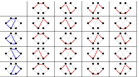
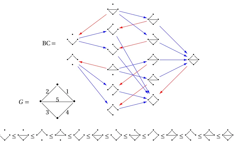
shows the set of diamonds (in blue) for the Bruhat order onS3. The maximal chain shown in rowd and columnC is the chaind Cdefined by the action of D(P)onCˆ0,ˆ1. . . 13 Figure 3.1 An example of the acyclic matching on BC for the graphG shown above, with

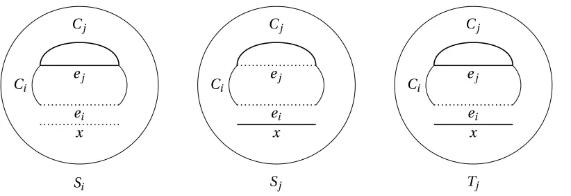
matched edges shown in red. Ranks are ordered reverse lexicographically from top to bottom. The resulting linear extension is shown below. . . 37 Figure 3.2 A schematic for visualizing the subgraphsSi,Sj, andTj. . . 38

Figure 4.1 (a) Thecapcobordism from_#to∅. (b) Thecupcobordism from∅to#. (c)

Thepantscobordism from_##to_#. (d) Thecopantscobordism from_#to

##. (e) The twist cobordism from_##to_##. . . 49 Figure 4.2 Axioms of a Frobenius algebra. The diagram on the right illustrates the

Frobe-nius relation. The other four diagrams illustrate the associativity, unit, coas-sociativity, and counit relations. . . 50 Figure 4.3 Equalities of cobordisms which correspond to axioms of Frobenius algebras

(compare to Figure 4.2). The equality at the top right corresponds to the Frobenius relation, and the equality at the bottom right guarantees that the corresponding Frobenius algebra is commutative. The other four equalities correspond to the associativity, unit, coassociativity, and counit relations. . . . 51 Figure 4.4 The defining relation of a special Frobenius algebra (Definition 4.2.1),

ex-pressed in terms of the corresponding TQFT. One may interpret this as the fact that special 2D TQFTs (those corresponding to special Frobenius algebras) do not detect genus (see Lemma 4.2.4). . . 52 Figure 4.5 A colored cobordism in (a) and a non-example in (b). . . 53 Figure 4.6 The 0 and 1 smoothings of a crossing in a knot diagram. . . 55 Figure 4.7 In (a), a diamond in the Bruhat order and in (b) the corresponding labelings

ofVD. . . 55

Figure 4.8 In (a) and (b) we see the two possible diamonds which can appear in case 1. In (c) we see the only possible type of diamond which can appear in case 2. . 56 Figure 4.9 A shortcut notation for colored cobordisms, as explained in 4.3.5. The above

picture denotes the cobordismC213,312_fromD213_toD312_whereD=T

2,3. . . . 57 Figure 4.10 Shown above is the diagram forVDin the case thatD is a diagram of the torus

Figure 4.11 (a) The diagramT2,n. (b) A smoothing ofT2,nwith height 1. (c) The smoothing

~α0_{gotten by changing the first 1 in~αto 0. (d) The smoothing~αfrom the proof} of Lemma 4.3.7. . . 58 Figure 5.1 Generators and their inverses for the braid groupBs. . . 62

Figure 5.2 A braid diagram and its braid closure. . . 62 Figure 5.3 In (a) we have the integral Khovanov homology ofT(3, 3n). In (b) we have the

integral Khovanov homology ofT(3, 3n+1). . . 64 Figure 5.4 In (a) we have the integral Khovanov homology ofT(3, 3n+2). In (b) we have

the integral Khovanov homology of the braid closure of∆2n+1. . . 64 Figure 5.5 Conventions for crossings and smoothings in link diagrams. . . 65 Figure 5.6 LV-indecomposable submodules ofH_<[i_∞,j](L). . . 73 Figure 5.7 Left: The braid wordω=∆2σ₁2σ2σ1∈Ω6and the corresponding diagram

φ(ω) =∆2_σ2

2σ1σ2. Think ofφ(D)asDrotated about the dotted line. Right: The braid wordωand its mirror imagem(ω). . . 77 Figure 5.8 TheF-Khovanov homology of the braid closure of∆2n+1overF=QorZp for

p an odd prime. . . 80 Figure 5.9 In (a) we have theZ2-Khovanov homology for the three component torus link

T(3, 3n). Each blue or green box represents a copy ofZ2which is killed in the Turner spectral sequence. In (b) we have theQ-Khovanov homology for the

torus linkT(3, 3n). Each blue or green box represents a copy ofQwhich is

killed in the Lee spectral sequence. . . 81 Figure 5.10 In (a) we have theZ2-Khovanov homology for the torus knotT(3, 3n+1).

Each blue or green box represents a copy ofZ2which is killed in the Turner spectral sequence. In (b) we have theQ-Khovanov homology for the torus

knotT(3, 3n+1). Each blue or green box represents a copy ofQwhich is killed

in the Lee spectral sequence. . . 82 Figure 5.11 In (a) we have theZ2-Khovanov homology for the torus knotT(3, 3n+2).

Each blue or green box represents a copy ofZ2which is killed in the Turner spectral sequence. In (b) we have theQ-Khovanov homology, andE1page of

the Lee spectral sequence, for the torus knotT(3, 3n+2). Each blue or green box represents a copy ofQwhich is killed in the Lee spectral sequence. . . 83

Figure 5.12 In (a) we have theZ2-Khovanov homology for the two component link∆2n+1. Each blue or green box represents a copy ofZ2which is killed in the Turner spectral sequence. In (b) we have theQ-Khovanov homology for the link ∆2n+1_{. Each blue or green box represents a copy ofQwhich is killed in the} Lee spectral sequence. . . 84 Figure 5.13 In (a) we have the rational Khovanov homology of the closure of the 3-braid

∆2_σ−5

1 ∈Ω4. In (b) we have the mod 2 Khovanov homology of the closure of the 3-braid∆2σ−5₁ ∈Ω4. Theorem 5.3.4 can not be applied here due to the mod 2 homology being supported on 3 diagonals in homological degree 0. In (c) we have the rational Khovanov homology of the closure of the 3-braid

∆2_σ2∈Ω

Figure 5.14 In (a) we have the rational Khovanov homology of the closure of the 3-braid

∆4_σ−2

CHAPTER

1

INTRODUCTION

Categorification can be thought of as something like a mathematician’s version of Plato’s allegory of the cave. In Plato’s allegory, a group of prisoners are confined in a dark cave facing a blank wall. Outside the cave, there is a fire which casts 2D shadows on the cave wall as 3D objects (birds, deer, etc...) pass by. The prisoners have no understanding of 3D objects and are aware only of the motions of the shadows on the wall. Plato’s idea of a philosopher is “one who escapes the cave” and learns the true nature of these 3D objects. With this allegory in mind, one might venture to imagine that many of the familiar mathematical objects in our experience are really “shadows” of some more structured objects hidden from our view. This is the idea of categorification. Inspired by the ideas of Crane and Frenkel[CF94], we now attempt to “escape the cave".

categorification

sets categories

elements objects

equations between isomorphisms between

elements objects

functions functors

equations between natural transformations functions between functors

decategorification

Figure 1.1An analogy between set theory and category theory taken from[BD98]. We can think of a set as a 0-category and a category as a 1-category. More generally, categorification should replace anncategory by an(n+1)category.

given object, but some ways may be more useful/natural than others. The “right" categorification should be one that not only lifts structures present at the decategorified level, but also introduces interesting new structures. We now provide some standard examples of categorification. Examples 1.0.1 and 1.0.2 can be thought of as the basic building blocks for more interesting categorifications such as Examples 1.0.3 and 1.0.4. Here, we keep the discussion somewhat informal, but these ideas can be made precise with the concept of the Grothendieck group (see Theorem 2.6.1, Example 2.6.2 and Example 2.6.3).

Example 1.0.1. The natural numbers(N,+,·)form the structure of arig, that is, a ring without

necessarily having additive inverses. The rig(N,+,·)is categorified by the category|-Vectof finite

dimensional vector spaces over a field|. Decategorification is done by taking the dimension of the

vector space: Decat(V) =dim(V). Direct sums and tensor products of vector spaces behave nicely in this regard: dim(V ⊕W) =dim(V) +dim(W)and dim(V ⊗W) =dim(V)dim(W). More precisely,

(N,+,·)can be recovered from(|-Vect,⊕,⊗)as the collection of isomorphism classes of objects in |-Vectwith operations[V] + [W] = [V ⊕W]and[V]·[W] = [V ⊗W]. The category|-Vectsatisfies

all of the appropriate coherence conditions needed to categorifyNas a rig, and for this reason is

called arig category. Not only are the usual properties of the natural numbers lifted to the category of vector spaces, but upon categorification, we introduce a variety of useful new tools and structures unavailable at the decategorified level (that is, all of linear algebra!).

An alternative way to categorify(N,+,·)is with(FinSet,q,×)whereFinSetis the category of

to show two natural numbersn,m ∈ Nare equal, combinatorialists like to find setsN andM

with cardinalitiesnandmrespectively, and show thatN andM are isomorphic (in this category, isomorphic means “in bijection with”).

Example 1.0.2. The ring(Z,+,·)of integers is categorified by the categoryCb(|-Vect)of bounded

chain complexes of|-vector spaces. Integers are categorified by chain complexesV∗where de-categorification is done by taking the Euler characteristic of a chain complex Decat(V_∗) =χ(V_∗) = P

n∈Z(−1)

n_dim(V

i)∈Z. Again, direct sums and tensor products behave as desired:χ(V∗⊕W∗) = χ(V_∗) +χ(W_∗)andχ(V_∗⊗W_∗) =χ(V_∗)χ(W_∗). The categoryCb(|-Vect)satisfies all of the

appropri-ate coherence conditions needed to cappropri-ategorifyZas a ring. Again, upon categorification, we have

introduced some very useful additional structure not available at the decategorified level (that is, all of homological algebra!). In the same manner, we can think of integers as being categorified by cochain complexesV∗(as opposed to chain complexesV_∗). Note that in this example and the previous one,|-Vectcan be replaced with the categoryR-modof finitely generated modules over a

commutative ringR(in this case dim should be replaced by rank).

In the previous two examples, we see categorifications ofNas a rig and ofZas a ring. As of

yet, there is no known categorification ofQorRas rings. As a step in this direction, Khovanov

and Tian give a categorification ofZ[12]in[KT17]. Next, we give two classical examples of novel categorifications, both providing a rich variety of new tools and structures in their respective fields. Example 1.0.3. LetSimdenote the category of simplicial complexes and simplicial maps, and let

∆∈Ob(Sim). Letfn(∆)denote the number ofndimensional faces in∆. The Euler characteristic χ(∆) =P

n≥0(−1)nfn(∆)is categorified by the simplicial homologyH∗(∆)of∆in the sense that X

n≥0

(−1)ndimHn(∆) =χ(∆). (1.1)

For this reason, given a chain complexC_∗, the quantityP_n∈Z(−1)ndimCn=

P

n∈Z(−1)

n_dimH n(C∗) is called the Euler characteristic ofC_∗. Simplicial homology contains the information of the Euler characteristic, but also has much more information about the space. For example, each homology groupHn(∆)is a topological invariant, and the rank of the homology groupHn(∆)indicates the

number of ‘holes’ of dimensionnin∆(see for example[Hat02, Chapter 2]).

The Euler characteristic of simplicial complexes is just a functionχ : Ob(Sim)→Zwhereas

homology is a functor H_∗ : Sim → Z-gmod, whereZ-gmod denotes the category of gradedZ

Example 1.0.4. A more recent example of categorification is the Khovanov homology of a knot/link. Khovanov homology is a bigraded Abelian group which categorifies the Jones polynomial of a link in the sense that one may recover the Jones polynomial by taking the (graded) Euler characteristic of the Khovanov homology. One can find details of this construction in Chapter 5 of this thesis. This theory was developed by Khovanov in[Kho00], with a more topological interpretation featured in the work of Bar-Natan in[BN05], and a more combinatorial construction featured by Viro in [Vir04]. The Jones polynomial is a powerful link invariant, and the Khovanov homology is a strictly stronger link invariant. Moreover, Khovanov homology can be shown to be functorial, meaning that a cobordism between links induces maps between the Khovanov homologies of those links. In particular this functoriality has proven useful in producing a lower bound for the slice genus of a knot (see[Ras10]). Rasmussen used this fact in[Ras10]to give a combinatorial proof of the Milnor conjecture, computing the slice genus of torus links.

The success of Khovanov’s categorification of the Jones polynomial has inspired many other categorifications. For example, Ozsváth and Szabó’s categorification of the Alexander polynomial in[OS04]done independently by Rasmussen in[Ras03]. In fact, there is a whole family{Pn}n∈N

of polynomial link invariants (including the Jones polynomialP2, and the Alexander polynomial P₀, as special cases) which are categorified by bigraded homology theories[KR04]. Khovanov and Rozansky’s categorification of the HOMFLY-PT polynomial (developed in [KR08]and [Kho07]) requires a triply-graded link homology theory. Similar in spirit to these theories, are Helme-Guizon and Rong’s categorification of the chromatic polynomial in[HGR05], Hepworth’s categorification of the magnitude of a graph in[HW15], Sazdanovi´c and Yip’s categorification of the Stanley chromatic symmetric function[SY18], Stˇosi´c’s categorification of the dichromatic polynomial[Sto08], and many more. Chapter 2 of this thesis is dedicated to this approach to categorification and outlining its use in the most general setting possible.

The theme of this thesis is categorification. In particular, categorification using the technique outlined by Khovanov in his categorification of the Jones polynomial. In the construction of Kho-vanov homology, KhoKho-vanov lifts a state sum formula for the Kauffman bracket (a rank-alternating sum over the Boolean lattice) to a functor on the Boolean lattice (viewing the Boolean lattice as a category). From this functor, he obtains a chain complex, and thus a homology theory. This homol-ogy theory categorifies the Kauffman bracket (and hence the Jones polynomial) in the sense that we recover the Kauffman bracket by taking its graded Euler characteristic. We generalize his approach by replacing the Boolean lattice by a broader class of posets under which this technique works. Thus we equip ourselves with the ability to categorify a broader class of invariants, those which admit rank alternating sums over thin posets. This broader class of posets is known as the class ofthin posets.

CHAPTER

2

THIN POSETS, CW POSETS, AND

CATEGORIFICATION

In 2000, Khovanov[Kho00]categorified the Jones polynomial by lifting Kauffman’s ‘state sum’ formula (a sum over a Boolean lattice) to a homology theory built from a functor on the Boolean lattice. This construction was further explained and popularized soon after by Bar-Natan[BN02]and Viro[Vir04]. Since Khovanov’s categorification, many authors have used similar techniques to categorify other polynomials which admit state sum formulas over Boolean lattices (see for example[HGR05; SY18; DL15; HW15; Sto08]). In this chapter, we set out a general framework for a larger class of posets, called thin posets (containing Boolean lattices as a special case), in which this categorification technique can be applied.

functors on thin posetsP requires the use of a so-called balanced coloring onP, that is, a{1,−1} coloring of the cover relations inP which plays nicely with the ‘thin structure’ inP (see Definition 2.3.5). However, balanced colorings on thin posets are not unique. The second main result in this chapter is Theorem 2.5.4, where we show that for diamond transitive thin posets, the homology theory obtained from a given functor is independent of the choice of balanced coloring. The proof of Theorem 2.5.4 depends on a topological interpretation of the property of diamond transitivity. In particular, we define a regular CW complexX(P)whose 1-skeleton is the Hasse diagramH(P), and show in Theorem 2.3.4 that ifP is diamond transitive, thenX(P)is simply connected.

In this thesis, we concern ourselves with topological/combinatorial invariants of spacesXwhich are related to the incidence ordering in the collection of cellsF(X)in some cell decomposition of those spaces, namely, those which admit formulas of the typeP_e∈F(X)(−1)dim(e)_{f(e)wheref :} F(X)→R is a function to some ringR. For example, Euler characteristics, h-polynomials, Tutte polynomials, and Jones polynomials all arise in this form. Notice these formulas (which we shall call rank alternators) do not depend on the partial order onF(X)in any way. In this context, categorification can be thought of as the process of upgrading these invariants in such a way that the partial order is taken into account. The next main result of this chapter is Theorem 2.6.6, where we outline how to categorify such invariants using functors on thin posets. The last main result of this chapter is Theorem 2.7.7, where we use algebraic Morse theory to simplify the calculation of the homology theory coming from a functor on a thin poset, given that the Hasse diagram of the poset has an acyclic matching for which the functor in question assigns isomorphisms to each edge in the matching.

We begin with a review of some needed terminology and notations from the theory of partially ordered sets. Nearly all of the material in Section 2.1 is standard and can be found in[Sta98]. For the more obscure material, citations will be provided along the way.

2.1

Background on Partially Ordered Sets

Apartially ordered set(orposet) is a setP together with a reflexive, antisymmetric, transitive relation, denoted≤P (or just≤ifP is understood). All posets in this thesis are assumed to be finite. A poset

P istotally orderedif for allx,y ∈P,x ≤y or y ≤x. Alinear extensionof a poset(P,≤)is a total order(P,≤0)onP with the property thatx≤y impliesx≤0y for allx,y ∈P. Ifx≤y andx6=y we writex<y. IfP has a unique minimal (respectively maximal) element, we denote this element by ˆ0 (respectively ˆ1). Alower order idealinP is a subsetLofP with the property that ify ∈Landx≤y thenx∈L. A mapf :P →Qbetween posets isorder preservingifx≤P y impliesf(x)≤Q f(y)for

f :P0→P. A subposetP0isinducedif f :P0→P is an order embedding.

Acover relationin a poset is a pair(x,y)∈P ×P withx ≤y such that there is noz ∈P with x<z <y, and in this case we writexly. LetC(P)denote the set of all cover relations inP. The

Hasse diagramof a finite poset is the directed graph(P,C(P))with nodesP and a directed edge drawn from left to right fromxtoy if and only ifxly (Hasse diagrams are normally drawn bottom

up, but in this thesis we draw them from left to right as this convention will be more useful for the construction of homology theories). We will call a posetconnectedif its Hasse diagram is connected. Achainin a posetPis a totally ordered subposetC ⊆P. We say that a chainCisfrom x to y ifx(resp. y) is the smallest (resp. largest) element ofC. A chain inP issaturatedif every cover relation inC is a cover relation inP. A chain ismaximalif it is not properly contained in any other chain. Equivalently, a maximal chain is a saturated chain from a minimal element ofP to a maximal element ofP.

Anabstract simplicial complexis a collection∆of subsets of a fixed finite setV (called the vertex set) such that ifF ∈∆andE ⊆F, thenE ∈∆. Each element of∆is called afaceof∆. The geometric realizationof∆is gotten by embedding the vertex set as an affinely independent set inRn

for large enoughn, and taking the union of the convex hulls of eachF ∈∆(this is well defined up to homeomorphism). Given a posetP, theorder complex,∆(P), is the abstract simplicial complex whose faces are the chains inP. That is,∆(P) ={F ⊆P |F is totally ordered}. One should note that we always have∅∈∆(P).

A posetP isgradedif there is a function rk :P →Nwith the property thatxly implies rk(y) =

rk(x) +1. Given a graded posetP, therankofP, denoted rk(P), is the maximum length of any chain inP, where the length of a chainC is defined as|C| −1. IfP has ˆ0, we will always assume that rk(ˆ0) =0, and so in this case, we will have rk(P) =max{rk(x)|x∈P}. IfPis a graded poset, andx≤y inP, thelengthof the interval[x,y] ={z∈P |x≤z ≤y}is rk(y)−rk(x). Equivalently, the length of

[x,y]is the length of any saturated chain fromxtoy.

Definition 2.1.1([Bjö84, Section 4]). A graded posetP isthinif every closed nonempty interval of length 2 has exactly 4 elements. In a thin poset, a closed nonempty interval of length 2 is called a diamond.

Remark 2.1.2. There is another class of posets referred to as thin posets in[BM11]. The above definition of thin posets is taken from[Bjö84]and has nothing to do with the one given in[BM11]. We now give a class of examples which we will make heavy use of throughout this thesis. In every example involving the concept of a ‘face poset’ we will always assume the existence of the ‘empty face’ which is contained in every other face, thus such posets will always have unique minimal elements ˆ0. IfP is a poset with ˆ0, we will often write ¯P =P\ {ˆ0}.

length 2 is of the form{T,T ∪ {x},T ∪ {y},T ∪ {x,y}}. See Figure 2.1 for an example of the Hasse diagram of a Boolean lattice.

Example 2.1.4. Let∆be anabstract simplicial complex. Theface posetof∆is the posetF(∆), with underlying set∆, partially ordered by inclusion. Every interval inF(∆)is isomorphic to a Boolean lattice, and therefore face posets of abstract simplicial complexes are also thin posets. Since the face poset of a simplex is itself a Boolean lattice, Example 2.1.3 is a special case of this example. The reader is referred to[Koz07, Section 2.1]for background information on abstract simplicial complexes and face posets if needed. Simplicial complexes give an effective way to study topological spaces using combinatorial methods due to the following fact: Given a topological spaceX, suppose there is a simpicial complex∆such that||∆||is homeomorphic toX. In this case,∆is referred to as atriangulationofX. Then the homeomorphism type ofX is determined by the posetF(∆)in the sense thatX ∼=∆(F(∆)). In fact, the order complex∆(F(∆))is the barycentric subdivision of∆(see for example[Wac06, Section 1]).

Example 2.1.5. LetΓ be apolyhedral complex, that is, a collectionΓ of polyhedra inRnfor somen

such that:

1. ifF ∈Γ andE is a face ofF, thenE ∈Γ,

2. the intersection of any two polyhedra inΓ is a face of each.

See[Koz07, Section 2.2]for background information on polyhedral complexes if needed. Theface posetofΓ is the posetF(Γ)with underlying setΓ, partially ordered by inclusion. Notice that the face poset of a polyhedral complex consisting of a single simplex (and all of its faces) is a Boolean lattice. Thus, Example 2.1.4 is a special case of this example. See Figure 2.1 for an example of the Hasse diagram of a polytopal complex (in this case, just a single polygon).

Example 2.1.6. For any Coxeter groupW, the Bruhat order Br(W)is a graded poset, with rank function given by the length of a reduced word. See[BB06, Section 2]for background information on the Bruhat order if needed. Björner noted in[BB06, Lemma 2.7.3]that Br(W)is a thin poset. Example 2.1.7. Recall aballin a topological spaceX is a subspaceBofX such thatB is homeo-morphic to the subspace{x ∈Rd : |x| ≤1}ofRd for somed. Theinteriorof a ball is the image

of{x ∈Rd : |x|<1}under such a homeomorphism. LetX be a Haussdorff space with aregular

CW decomposition,Γ. That is,Γ is a collection of closed balls inX such that the interiors of balls inΓ partitionX, and for each ballσ∈Γ of positive dimension, the boundary∂ σis a union of balls inΓ. In this case,Γ is called aregular CW complex, and one will often write||Γ||=∪σ∈Γσso in

are defined by specifying attaching maps to glue balls of different dimensions together. One may alternatively define regular CW complexes as those CW complexes whose attaching maps are all homeomorphisms.

Given a regular CW complexΓ, itsface poset,F(Γ), is the poset with underlying setΓ, partially ordered by containment. See[BB06, Appendix A2.5]or[Bjö84]for background information on regular CW complexes and their face posets. It was noted by Björner that face posets of regular CW complexes are thin[Bjö84, Proposition 3.1 and Figure 1(a)]. This is not true in general for face posets of CW complexes. Following the terminology in[Bjö84], we will refer to face posets of regular CW complexes asCW posets. See Definition 2.1.8 for a poset theoretic definition and Theorem 2.1.9 to see that the two definitions are equivalent. As shown in[Bjö84, Section 2], Examples 2.1.3, 2.1.4, 2.1.5 and 2.1.6 are all special cases of face posets of regular CW complexes. From the perspective of a combinatorialist interested in topology, regular CW complexesΓ are important because the combinatorics ofF(Γ)determines the topology of||Γ||in the sense that||Γ|| ∼=∆(F(Γ))[BB06, Fact A.2.5.2]. This is not true in general for face posets of CW complexes. Thus regular CW complexes can be thought of as those CW complexes which can be completely understood combinatorially. Definition 2.1.8([Bjö84, Definition 2.1]). ACW posetis a posetP with ˆ0, and at least one other element, for which any open interval of the form(ˆ0,x)is homeomorphic to a sphere (that is, the order complex∆(ˆ0,x)is homeomorphic to a sphere).

The following properties of CW posets are proven in[Bjö84]Proposition 2.6, Figure 1(a), and Sections 2.3-2.5.

Theorem 2.1.9([Bjö84]). Let P be a finite poset.

1. P is a CW poset if and only if P is a face poset of a regular CW complex.

2. If P is a CW poset then P is thin.

3. If P is a CW poset and L is a lower order ideal in P , then L is a CW poset.

4. If P is a CW poset and x ∈P , then{y ∈P |y ≥x}is a CW poset.

5. Face posets of simplicial complexes, Bruhat orders on Coxeter groups, and face posets of polytopal complexes are all CW posets.

2[3] Br(S3) F( )

∅

{1} {2} {3}

{1, 2} {1, 3} {2, 3}

{1, 2, 3}

Boolean lattices

123 213

132 231

312 321

Bruhat orders

•

• • • • • •

• • • • • •

•

Face posets of polytopes

Figure 2.1In this figure we see the Boolean lattice 2[3]_{consisting of all subsets of[3] ={1, 2, 3}(or} equiva-lently the face poset of the 2-simplex), the Bruhat order on the symmetric groupS3, and the face poset of a

hexagon.

2.2

The Diamond Group and Diamond Transitivity

Given a thin posetP, letSdenote the set of diamonds inP (see Definition 2.1.1). LetW(P)denote the group with presentation〈S |R〉, whereR ={d2_{|d ∈S}. Givenx,y ∈P withx ≤y, letC}

x,y

denote the set of all maximal chains in the interval[x,y]and letCP (or justC whenP is understood)

denote the disjoint union of all of the setsCx,y for each pair(x,y)wherex≤y inP. In other words,

C =CP is the set of all saturated chains inP.

Definition 2.2.1. Given a diamondd={x,a,b,y} ∈S(wherex_la_ly andx_lb_ly) and a saturated chainC ∈ C, defined C∈ C as follows:

• Ifxlaly is a subchain ofC, defined C= (C \ {a})∪ {b},

• Ifxlbly is a subchain ofC, defined C = (C\ {b})∪ {a},

• Otherwise, defined C=C.

We will refer to the process of passing fromC tod Cas performing adiamond moveonC.

Intuitively, ifC contains one side of the diamondd, we formd C by reroutingC along the other side of the diamondd. Notice that for anyd ∈S, and anyC ∈ C,d(d C) =C, and therefore this defines an action ofW(P)onC via(d1. . .dk−1dk)(C) =d1(. . .dk−1(dk(C)). . .). LetN(P)denote the

subgroup ofW(P)generated by all words which act trivially onC. The following two facts are special cases of a more general well known result, but we provide proofs here for convenience.

Lemma 2.2.2. For any thin poset P with diamond set S , N(P)is a normal subgroup of W(P).

Proof. Letw∈N(P),y ∈W(P), andC ∈ C. Then

Thereforey−1w y∈N and we conclude thatN(P)is normal.

Definition 2.2.3. Given a thin posetP, thediamond group,D(P)is defined as the quotient ofW(P) by the normal subgroupN(P):

D(P) =W(P)/N(P).

Recall, a group action is calledfaithfulif the only element ofG which fixes every element ofX is the identity element.

Lemma 2.2.4. Given a thin poset P , D(P)acts faithfully on the setC of saturated chains.

Proof. Givenw∈W(P)let us denote the class ofwinD(P)by[w]. The action ofW(P)onC decends to an action ofD(P)onC via[w]C =w C. This is well defined since if[w] = [v], thenw−1v∈N(P) and thusw−1vacts trivially on all elements ofC. Therefore, for allC ∈ C,w C =w(w−1v)(C) =v C. This is a group action since[v]([w]C) =v(w C) = (v w)(C) = ([v w])C = ([v][w])C for allv,w∈W(P) andC∈ C. Suppose[w]∈D(P)satisfies[w]C =C for allC ∈ C. Thenw C=C for anyC ∈ C and thereforew ∈N(P)and therefore[w]is the identity element inD(P).

Recall that if a groupG acts on a setX, andY ⊆X is a subset which is closed under the action ofG, thenG also acts onY by restriction. In our case, notice that for eachx≤y,Cx,y ⊆ C is closed

under the action ofD(P). An action ofG onX is calledtransitiveif for anyx,y ∈X there exists g∈G such thatg x=y. In other words, if we letOx={g x|g∈G}denote theorbitofxunder the

action ofG, thenG acts transitively onX ifX =Ox for some (equivalently for all)x∈X.

Definition 2.2.5. A thin posetP isdiamond transitiveifD(P)acts transitively onCx,y for each pair (x,y)such thatx≤y inP.

Example 2.2.6. LetP=Br(S3) =• • • • • • , S= ¨ • • • • • • , • • • • • • , • • • • • • , • • • • • • « and Cˆ0,ˆ1= ¨ • • • • • • , • • • • • • , • • • • • • , • • • • • • « . ThenD(P)acts onCˆ0,ˆ1according to the table in Figure 2.2.

We now give a characterization of small intervals in diamond transitive thin posets.

• • • • • • • • • • • • • • • • • • • • • • • • • • • • • • • • • • • • • • • • • • • • • • • • • • • • • • • • • • • • • • • • • • • • • • • • • • • • • • • • • • • • • • • • • • • • • • • • • • • • • • • • • • • • • • • • • • • • • • • • • • • • • • • • • • • • • • • • • • • • • • • •

Figure 2.2The top row shows the set of maximal chains (in red), and the leftmost column shows the set of diamonds (in blue) for the Bruhat order onS3. The maximal chain shown in rowd and columnC is the

chaind Cdefined by the action ofD(P)onCˆ0,ˆ1.

•

•

•

•

Intervals of length 2

• • • • • • • • • • • • .. . ...

Intervals of length 3

Proof. The result for intervals of length 2 follows from thinness. Consider now an interval[x,y]of length 3 in a diamond transitive thin poset. Take a chain of the formxla0lb0ly in[x,y]. The

interval[x,b0]must be a diamond, so there must bea16=a0∈P withxla1lb0. The interval[a1,y] must be a diamond, so there must be an elementb₁6=b₀∈P witha_1lb_1ly. The interval[a₀,y] must be a diamond so eithera0lb1or we continue the process by adding elementsa2,b2with a2lb1anda2lb2. SinceP is finite, one must eventually stop adding such elementsai,bi. Now, the

interval[x,b₀]must be a diamond, so eventually we must connecta₀tob_k for somek.

Once we reachk such thata0lbk, we claim there can be no more elements in[x,y]besides

those already considered. Suppose there were some elementak+1in[x,y]withxlak+1. Ifak+1lbi

for somei ≤k then thinness is contradicted so there must be someb_k+1witha_k+1lbk+1ly. If

ailbk+1for anyi≤k then again thinness is contradicted. However now, there is no way to get to the chainxlak+1lbk+1ly from the chainxlaklbkly by diamond moves, thus contradicting

diamond transitivity. Thus every interval of length 3 is of the combinatorial type shown in the statement above.

diamond transitive thin posets and CW posets. As a partial answer to this, Theorem 2.4.12 tells us that all CW posets are diamond transitive. Conjecture 2.8.1 surmises a partial converse to this.

The following theorem, while less general than the forthcoming Theorem 2.4.12, provides an opportunity to present a direct proof of diamond transitivity.

Theorem 2.2.9. Face posets of simplicial complexes are diamond transitive.

Proof. LetP be the face poset of a simplicial complex. Recall intervals in face posets of simplicial complexes are Boolean lattices. Consider an interval[x,y]inP. Then by the above remark,[x,y]∼₌ 2[n]for somen. The set of elements in 2[n]of a given rank (that is, all subsets of[n]of a given size) can be totally ordered lexicographically, and this induces a lexicographic on maximal chains. LetC0 denote the lexicographically largest chain∅⊆ {n} ⊆ {n−1,n} ⊆ · · · ⊆[n].

We now show, by induction on the distanced(C,C0)in lexicographic order betweenC andC0 that there existsw∈D(P)such thatw C=C₀. The base case is trivial since for distance 0 we have C =C0. Otherwise, sinceC is not lexicographically largest, there is a subchainS⊆S+i⊆S+i+jof C withi<j. Now consider the (lexicographically larger) chaind Cwhered={S,S+i,S+j,S+i+j}. By induction we havew∈D(P)such thatw(d C) =C₀= (w d)C.

2.3

The Diamond Space and Balanced Colorability

In this section, we give a topological interpretation of diamond transitivity. This interpretation turns out to be useful in regard to understanding certain{1,−1}colorings (called balanced colorings) of the cover relations ofP, which we use in Section 2.5 to define homology theories.

Definition 2.3.1. Given a thin posetP, we construct a regular CW complexX(P)as follows: 1. The 0-skeleton,X0_{(P)ofX(P)is the setP.}

2. The 1-skeleton,X1_{(P)ofX(P)is the (undirected) Hasse diagram ofP, that is, we glue in a} 1-cell connecting pairs(x,y)wheneverxly.

3. The 2-skeletonX2(P) =X(P)ofX(P)is gotten by gluing 2-cells into each diamond inP. Since we will add no higher dimensional cells,X(P)is equal to the 2-skeleton.

Call the resulting regular CW complexX(P)thediamond spaceofP.

LetP be a thin poset. Fix a continuous mapφ:X1(P)→R, so that for eacha∈X0(P),φ(a) =

rk(a), and on each closed 1-celle inX1_{(P), corresponding to an edge inH(P)fromatob,φ|}

e is a

Definition 2.3.2. Letr1,r2∈R. A continuous mapγ:[r1,r2]→X1(P)ismonotonically increasing (resp.monotonically decreasing) if for alls,t ∈[r1,r2],s<t impliesφ(γ(s))< φ(γ(t))(resp.φ(γ(s))> φ(γ(t))).

Lemma 2.3.3. Let P be a diamond transitive thin poset withˆ0. Any continuous mapγ:[0, 1]→X(P) withγ(0) =γ(1) =ˆ0is homotopic to a piecewise linear mapγ0:[0, 1]→X1_(P)withγ0_{(0) =γ}0_{(1) =ˆ0} such that there exists r ∈(0, 1)so thatγ0|[0,r]is monotonically increasing andγ0|[r,1]is monotonically decreasing.

Proof. Letγ:[0, 1]→X(P). Using the cellular approximation theorem[Hat02, Theorem 4.8], we see thatγis homotopic to a map ¯γwhose image is contained inX1_{(P). Then, by applying the simplicial} approximation theorem[Hat02, Theorem 2C.1]to ¯γ, we see thatγis homotopic to a map ˜γthat is simplicial with respect to some iterated barycentric subdivision of[0, 1]. In other words, there is a partition 0=r₀<r₁<· · ·<r₂k =1 of[0, 1]such that

1. ˜γ(r₀) =γ˜(r_2k) =ˆ0 2. ˜γ(ri)∈X0(P)for eachi

3. For 0≤i≤2k−1, ˜γ(ri)lγ˜(ri+1)or ˜γ(ri+1)lγ˜(ri)

4. Ifr ∈[0, 1]\ {r0, . . . ,r2k}then ˜γ(r)∈X1(P)\X0(P)

5. For 0≤i≤2k−1, ˜γis linear (in particular either monotonically increasing or decreasing) on

[ri,ri+1].

Choosei₁<· · ·<i_{2`</sub>where{i<sub>1</sub>, . . . ,i<sub>2`}} ⊆ {1, . . . , 2k}such that ˜γis monotonically increasing on[0,r_i1], monotonically decreasing on[ri1,ri2], monotonically increasing on[ri1,ri3]and so on. We will show

by induction on`(that is, half the number of subintervals in such a partition) that ˜γis homotopic to a mapγ0<sub>as desired in the statement of this lemma. If`=1, then ˜γmonotonically increases on</sub>

[0,ri1], and monotonically decreases on[ri1, 1], so we are done. If` >1 we proceed as follows. Recall

that pathsα,βcan be multiplied to form the product pathαβwhich traverses firstαand thenβ. Also recall that, given a pathα:[a,b]→X in a topological spaceX, we letα−1_{denote the path} defined byα−1:[−b,−a]→X whereα−1(t) =α(−t), soα−1traverses the same points asαbut in the opposite direction (see[Hat02, Section 1.1]). In the Hasse diagramH(P), ˜γ|[0,ri₁]corresponds to a

directed path from ˆ0 to some elementx₁∈P. Now,(γ|˜_[ri1,ri2])

−1_{corresponds to a directed path in} H(P)starting at some elementx2and ending atx1. Let ˆ0=y0ly1l· · ·lyn=x2be a directed path in H(P), and letβ:[0, 1]→X1(P)be a monotonically increasing piecewise linear map corresponding to this directed path. Thenβ(γ|˜_[ri1,ri2])

−1_{is piecewise linear and monotonically increasing from ˆ0 to} x1. SinceP is diamond transitive, there is a sequence of diamond moves taking the path ˜γ|[0,ri₁]to the pathβ(γ|˜_[ri

1,ri2])

side of the diamond to the path along the other side. Thus, ˜γ=γ|˜_[0,ri₁]γ|˜[ri₁,1]is homotopic to the pathβ(γ|[˜ _ri

1,ri2])

−1_γ|[˜

ri₁,1]which is homotopic toγ0=β(γ|[˜ ri₂,1]). Notice thatγ0has a partition of its

domain 0<ri3<· · ·<ri2`with 2(`−1)subintervals so thatγ0is monotonic on each subinterval. Thus

we are done by induction.

Theorem 2.3.4. Let P be a diamond transitive thin poset withˆ0. Thenπ1(X(P), ˆ0)is trivial.

Proof. Suppose thatP is diamond transitive. By Lemma 2.3.3, any loopγ:[0, 1]→X(P)based at ˆ0 can be homotoped to a loopγ0_{:[0, 1]→X}1_{(P)such that there existsr ∈(0, 1)for whichγ}0_|

[0,r] increases monotonically to some elementx∈P andγ0|[r,1]decreases monotonically fromx back to ˆ0. LetC1= (ˆ0=x0lx1l· · ·lxk=x)be the saturated chain inP corresponding toγ0|[0,r]and let C₂= (ˆ0=y₀ly1l· · ·lyk=x)be the saturated chain inP corresponding to(γ0|[r,1])−1. SinceP is diamond transitive, there is a sequence of diamond moves that takesC1toC2, and this defines a homotopy fromγ0|[0,r]to(γ0|[r,1])−1. Thusγ0is homotopic toγ0|[0,r](γ0|[0,r])−1which is homotopic to

the constant map at ˆ0. Thus we have shown that any loop inX(P)based at ˆ0 is nullhomotopic. Definition 2.3.5([BB06, Section 2.7]). Abalanced coloringon a thin posetP is a functionc:C(P)→ {1,−1}if each diamond inP is assigned an odd number of−1 colored edges. A thin posetP is balanced colorableif it admits a balanced coloring.

We have now seen a relationship between the combinatorial property of diamond transitivity inP to the topology of the spaceX(P). Next, we show that the property of balanced colorability can also be thought of in terms of the diamond spaceX(P). Balanced colorings ofP are{1,−1} colorings of the edges in the Hasse diagramH(P). Thus balanced colorings can be viewed as ele-ments of the cochain groupC1(X(P),Z2) =Hom(C1(X(P),Z2). Warning: the coefficient groups for cohomology are usually written with additive notation, however because of our situation, we will use multiplicative notation, identifying({0, 1},+)with({1,−1},·). Consider the functionφ0:C2(X(P))→

Z2={1,−1}sending every 2-cell to−1∈Z2. Recall, 2-cells correspond to diamonds inP, so we will denote 2-cells byd and each 2-cell has boundary consisting of four edges{e₁d,e₂d,e₃d,ed

4}. Given ψ:C1(X(P))→Z2,δψ:C2(X(P))→Z2is defined on 2-cellsd with boundary{e1d,e2d,e3d,e4d}by δψ(d) =ψ(e₁d)ψ(e₂d)ψ(e₃d)ψ(e₄d). Ifδψ=φ0, thenψ(e₁d)ψ(e₂d)ψ(e₃d)ψ(e₄d) =−1 for each diamond d, or in other words,ψis a balanced coloring. SinceX(P)has no 3-cells,φ0is guaranteed to be a cocycle. Since we are working over the fieldZ2, we haveHk(X(P),Z2)∼=Hom(Hk(X(P),Z2),Z2)for allk. Thus we have proven the following.

Proposition 2.3.6. Letφ0:C2(X(P))→Z2={1,−1}denote the cocycle sending every 2-cell to−1∈Z2. Then P is balanced colorable if and only if[φ0]is trivial in H2_(X(P),

Z2). In particular, this says that ifH2_(X(P),

Proposition 2.3.7. Let P be a thin poset and suppose that X(P)forms the 2-skeleton of a regular CW complex Z(P)in which each 3-cell has an even number of 2-dimensional faces, and suppose that H2_(Z(P),

Z2) =0. Then P is balanced colorable.

Proof. SinceX(P)andZ(P)have the same 2-skeleton, we have thatC2_(X(P),

Z2) =C2(Z(P),Z2) so we can identifyφ0as a 2-cochain inZ(P). LetF be a 3-cell inZ(P). By assumption,F has an even number of 2-dimensional faces,d1, . . . ,d2n. In our multiplicative notation (Z2={1,−1}) we haveδφ0(F) =Q2_i=1n φ0(di) = (−1)2n_{=1. Thereforeδφ0is the identity element inC}3_(Z(P),

Z2), so φ0∈C2(Z(P),Z2)is a cocycle. SinceH2(Z(P),Z2) =0,φ0is a coboundary. Thusφ0=δψfor some ψ:C1(Z(P))→Z2. SinceX(P)andZ(P)have the same 1-skeleton, we haveC1(X(P)) =C1(Z(P))so we can identifyψ:C₁(X(P))→Z2as a 1-cochain inX(P). Therefore we have that[φ0]is trivial in H2(X(P),Z2)and so by Propsitition 2.3.6,P is balanced colorable.

Example 2.3.8. As an easy application of Proposition 2.3.7, we see that the Boolean latticeBn is

balanced colorable sinceX(Bn)is the 2-skeleton of then-cube. Note that every 3-cell in an

n-cube is a 3-n-cube, and thus has an even number of faces. Khovanov makes use of such a balanced coloring in[Kho00, Section 3.3], en route to constructing a homology theory which categorifies the Jones polynomial. More generally, this argument shows that any poset whose Hasse diagram is the 1-skeleton of acubical polytopeis balanced colorable.

Definition 2.3.9. Given a thin posetP, acentral coloringofP is a mapd:C(P)→ {1,−1}such that every diamond has an even number of−1’s.

LetP be a thin poset, and letΦdenote the group of all edge coloringsf :C(P)→Z2={1,−1} of the Hasse diagram, with group operation defined by pointwise multiplication of functions. Let

Φb _{⊆Φdenote the set of balanced colorings and letΦ}c_{⊆Φdenote the set of central colorings.}

Lemma 2.3.10. If P is diamond transitive, then for any d∈Φc there exists f :P → {1,−1}such that δf =d .

Proof. SinceP is diamond transitive, it follows from Theorem 2.3.4 that we haveH1_(X(P),

Z2) =0. Sincec ∈Φc, we havec∈kerδ1=imδ0.

Lemma 2.3.11. For any c1,c2∈Φb, c1c2∈Φc.

Proof. Consider a diamond with edgese,f,g,h. Then

c1(e)c1(f)c1(g)c1(h) =−1 and

so

(c1c2)(e)(c1c2)(f)(c1c2)(g)(c1c2)(h) =1. Lemma 2.3.12. For any c1,c2∈Φb there exists d∈Φc such that c1d=c2.

Proof. Notice that for anyc∈Φ,c2=id_Φ. Letd=c1c2(an element ofΦc by Lemma 2.3.11). Then c₁d=c₁c₁c₂=id_Φc₂=c₂.

This homological interpretation of balanced colorings is utilized in Section 2.5, where we use balanced colorings to construct homology theories from thin posets. To conclude this section, we state a result of Björner, which also finds its utility in Section 2.5.

Theorem 2.3.13([BB06, Corollary 2.7.14]). CW posets are balanced colorable.

Proof. This follows from[BB06, Corollary 2.7.14]by noticing the proof is not specific to the Bruhat order, but holds for all CW posets.

2.4

CW posets and Obstructions to Diamond Transitivity

In this section, we begin by giving a way to construct thin posets which are not diamond transitive. We then show that this construction provides the only possible type of obstruction to diamond transitivity. This gives us a classification of diamond transitive posets in terms of obstructions, and this classification allows us to prove that all CW posets are diamond transitive.

Definition 2.4.1. Given two thin posetsP (with ˆ0P and ˆ1P) andQ(with ˆ0Qand ˆ1Q) of the same rank

n≥3, define thepinch product P• •Qby

P • •Q= (P− {ˆ0

P, ˆ1P})q(Q− {ˆ0Q, ˆ1Q})q {ˆ0, ˆ1}

whereqdenotes disjoint union. A partial order onP • •Qis defined by settingx≤y if any of the

following conditions hold: 1. x=ˆ0 ory =ˆ1,

2. x,y ∈P− {ˆ0P, ˆ1P}andx≤P y,

3. x,y ∈Q− {ˆ0Q, ˆ1Q}andx≤Q y.

In other words, the pinch product is formed by removing the ˆ0 and ˆ1 from each poset, taking the disjoint union, and then adding a new ˆ0 and ˆ1 to the result.

Proof. The pinch productP • •Qis graded with rank function

rk(x) =             

0 ifx=ˆ0

n ifx=ˆ1

rkP(x) ifx∈P− {ˆ0P, ˆ1P}

rkQ(x) ifx∈Q− {ˆ0Q, ˆ1Q}

Any interval of length two can be identified as either an interval of length two inP or an interval of length two inQand is thus a diamond.

Example 2.4.3. LetP=Br(S3)• •Br(S

3). The Hasse diagram ofP is shown below:

•

•

•

•

•

•

•

•

•

•

Notice the green chain and the red chain are in different orbits ofD(P), soPis not diamond transitive. In fact, it is not hard to see thatP is the smallest possible non-diamond transitive thin poset. This poset also appears in[Sta94, Figure 2]as an example of an Eulerian poset which is not a CW poset. It is not hard to see thatP is also the smallest possible thin poset with ˆ0 which is not a CW poset. Lemma 2.4.4. For any two thin posets P,Q,with ˆ0and ˆ1, of equal rank n ≥3, there is a group isomorphism f :D(P)×D(Q)→D(P • •Q)such that the following diagram commutes:

D(P)×D(Q) D(P • •Q)

S_CP ×S_CQ S_C

f

Proof. LetS(resp.SP,SQ) be the set of diamonds inP • •Q(resp.P,Q), and letC(resp.C

P,CQ) be the

set of saturated chains inP • •Q(resp.P,Q). ThenS=S

PqSQandC =CPqCQ. Furthermore notice

that ifd ∈SP ande∈SQ thatd e =e dinD(P • •Q). Therefore we can factorD(P • •Q) =D(P)×D(Q)

by writing any wordd1. . .dk ∈D(P)in the form(e1. . .er)(fr+1. . .fk)whereei∈SP andfj ∈SQ for all

i,j. We define the mapf by sending(e1. . .erf1. . .fs)∈D(P)×D(Q)toe1. . .erf1. . .fs ∈D(P • •Q).

Lemma 2.4.5. For any two thin posets P,Q,withˆ0andˆ1, of equal rank n≥3, P• •Q is not diamond

transitive.

Proof. Given a maximal chainC inP, a maximal chainC0inQ, andw∈D(P • •Q), the action of

f−1(w)onC gives another maximal chain inP, so by the commutative diagram in Lemma 2.4.4, w C 6=C0_{for anyw∈D(P} • •Q).

In what follows, given a subsetS of a poset(P,≤), we will automatically identifyS with the induced subposet ofP with underlying setSand partial order≤0defined for allx,y ∈Sbyx≤0y if and only ifx≤y. Given any interval[x,y]inP of length at least 2, the diamond groupD([x,y])acts on the set of maximal chains in[x,y]. Given a maximal chainC in[x,y](that is, a saturated chain fromx toy), letOC denote the orbit ofC with respect to this action. Given any saturated chainC,

defineP_C to be the induced subposet ofP with underlying set∪C0_∈OCC0.

Definition 2.4.6. An induced subposetS ofP issaturated if every saturated chain inS is also saturated inP.

Definition 2.4.7. A saturated subposetSofP isdiamond-completeif every for every diamondd in P, and every saturated chainC inS,d C ⊆S.

Lemma 2.4.8. For any saturated chain C in a thin poset P , PC is a diamond-complete thin subposet.

Proof. Every saturated chain inPC is a saturated chain inP by construction. Given a diamondd in

P and a saturated chainC0inPC,d C0∈ OC and therefored C0⊆PC by definition, soPC is diamond

complete. To see thatP_C is thin, suppose thatx<y inP_C and rk(y) =rk(x) +2. Sincex<y is not saturated inP, it must not be saturated inPC. Therefore there is an elementa∈PC withx<a<y.

Extend this to a maximal chainC0inPC. SinceP is thin, there exists another elementb∈P with

x<b<y, and consider the diamondd={x,a,b,y}. By definition ofP_C, all elements ofd C0_{are in} PC and thereforeb∈PC, so the interval[x,y]inPC consists of four elements{x,a,b,y}.

Lemma 2.4.9. Given x<y in P withrk(y)≥rk(x) +3, suppose C and D are saturated chains from x to y such thatOC 6=OD and PC∩PD={x,y}. Then PC ∪PD is a diamond-complete thin subposet

of P isomorphic to PC • •P

D.

Proof. First we show thatPC ∪PD is induced by induction on the length`ofC. The base case is for

`=3. In this case,C =xlc1lc2ly andD=xld1ld2ly. Suppose towards a contradiction that PC ∪PD is not induced. Then without loss of generality we must havec1ld2. However in this case,

(c1,y)consists of at least 3 elements, contradicting thinness ofP. Suppose now that` >3, and again suppose towards a contradiction thatPC ∪PDis not induced. In this case,C =xlc1l· · ·lc`−1ly

andD =xld1l· · ·ld`−1ly. Then without loss of generality there is a cover relationcildi+1 for some 1≤i≤`−2. LetC0_{denote the chainx}

xld1l· · ·ldildi+1. ThenPC0 is an induced subposet ofPC andPD0is an induced subposet of

PD. LetC00denote the chaincilci+1l· · ·l ly and letD00denote the chaincildi+1l· · ·ly. Then

PC00is an induced subposet ofPC andPD00is an induced subposet ofPD. By induction,PC0∪PD0and

PC00∪PD00are induced and meaning that there are no other cover relations betweenC andDbesides

cildi+1and possiblydilci+1. This contradicts thinness ofP since then we have(ci,di+2) ={di+1}.

We have thatPC∪PD is saturated since any saturated chain inPC∪PDis either a saturated chain

inPC or a saturated chain inPD, and so by Lemma 2.4.8, is saturated inP. Furthermore,PC∪PD

is diamond-complete since any saturated chain inPC ∪PD lies entirely inPC orPD respectively,

and thus by Lemma 2.4.9, any diamond move on such a chain gives another chain inPC orPD

respectively. Lastly,PC ∪PD is thin since any interval of length two inPC∪PDis either an interval of

length two inP_C or inP_Dand is therefore a diamond again by Lemma 2.4.8.

Theorem 2.4.10. Let P be a thin poset. Then P is diamond transitive if and only if P contains no diamond-complete subposet isomorphic to a pinch product of two thin posets.

Proof. IfP is not diamond transitive, one can find saturated chainsC andD fromx toy inP for some x,y ∈P such thatOC 6=OD andPC ∩PD ={x,y}. Lemma 2.4.9 then provides a

diamond-complete thin subposet isomorphic to a pinch product. Conversely, supposeP contains a diamond-complete subposet isomorphic to a pinch product, say of the formQ=Q₁• •Q

2with some unique minimal element ˆ0Q and maximal element ˆ1Q. LetC1⊆Q1andC2⊆Q2be a saturated chains from ˆ0Q to ˆ1Q inP. Note thatQ1andQ2 are diamond-complete by Lemma 2.4.8 sinceQ1=PC1 and

Q₂=PC2. For any sequence of diamondsd1. . .dr inP,(d1. . .dr)C1⊆Q1, soC1andC2are in different

orbits of the action ofD(P)and thereforeP is not diamond transitive.

In Remark 2.2.8 and Example 2.4.3, we noted that CW posets share certain similarities with diamond transitive thin posets. We now further explore this connection.

Proposition 2.4.11. If P can be written in the form P =P1• •P

2, where P1and P2are thin posets of equal rank, then P is not a CW poset.

Proof. SinceP has ˆ1, ifP is a face poset of a CW complexY, thenY must be connected. Suppose to the contrary thatP =P1• •P

2is the face poset of a regular CW complex. Removing the top element, P =P1• •P

2\ˆ1 is also the face poset of a regular CW complexX =X1qX2whereX1=P1\ˆ1 and X₂ =P₂\ˆ1. But there is no way to glue ann-cell to ann−1 dimensional skeleton which is not connected, and obtain a connected space (i.e. the image of a continuous mapf :en→X1qX2must be contained in eitherX1orX2).