DOI: 10.1534/genetics.105.043828
Quantitative Trait Locus Analysis of Longitudinal Quantitative Trait Data
in Complex Pedigrees
Stuart Macgregor,*
,†,1Sara A. Knott,* Ian White* and Peter M. Visscher*
,2*Institute of Evolutionary Biology, University of Edinburgh, Edinburgh EH9 3JT, United Kingdom and†Biostatistics and Bioinformatics Unit, Cardiff University, Cardiff CF14 4XN, United Kingdom
Manuscript received March 30, 2005 Accepted for publication July 7, 2005
ABSTRACT
There is currently considerable interest in genetic analysis of quantitative traits such as blood pressure and body mass index. Despite the fact that these traits change throughout life they are commonly analyzed only at a single time point. The genetic basis of such traits can be better understood by collecting and effectively analyzing longitudinal data. Analyses of these data are complicated by the need to incorporate information from complex pedigree structures and genetic markers. We propose conducting longitudinal quantitative trait locus (QTL) analyses on such data sets by using a flexible random regression estimation technique. The relationship between genetic effects at different ages is efficiently modeled using covariance functions (CFs). Using simulated data we show that the change in genetic effects over time can be well characterized using CFs and that including parameters to model the change in effect with age can provide substantial increases in power to detect QTL compared with repeated measure or univariate techniques. The asymptotic distributions of the methods used are investigated and methods for overcoming the practical difficulties in fitting CFs are discussed. The CF-based techniques should allow efficient multivariate analyses of many data sets in human and natural population genetics.
Q
UANTITATIVE traits such as cholesterol levels in humans, milk yield in dairy cows, and fruit size in tomatoes are known to change over time; they are inherentlylongitudinalin nature. A major aim of genetics is to better understand the composition of such traits. With the advent of inexpensive molecular marker tech-nology a wide variety of quantitative trait locus (QTL) mapping techniques have been developed to allow the dissection of quantitative traits in outbred populations(e.g., Hasemanand Elston1972; Goldgar1990; Amos
1994; Hoeschele et al. 1997; Almasy and Blangero
1998; Georgeet al.2000). While these allow the
ex-traction of information from univariate data (one trait measure per individual), techniques for QTL mapping when there are multiple trait measures are less well developed.
Existing univariate techniques can be readily applied to data measured at different stages of life but such ap-proaches fail to capture the correlations between the components underlying traits such as cholesterol. At the other extreme, analyses are readily performed if we are prepared to assume that there is no change in the ge-netic composition of the trait over life [i.e., that the measures made are simply repeated realizations of
ex-actly the same trait (Lynchand Walsh1998)]. Neither
of these approaches is satisfactory for many traits. A further alternative involves treating the individual trait measures (taken at different times) as distinct trait measures and modeling the covariance between the different traits in a multivariate analysis (e.g., Eaveset al.
1996). Such techniques, however, are difficult to apply in practice, may involve too many parameters in the model, and do not take the time element into account. Ideally longitudinal traits would be modeled allowing for the fact that the multiple measures are ordered in time. To address this, Kirkpatricket al.(1990)
intro-ducedcovariance functions(CFs) to describe the relation-ship between different ages; CFs are simply continuous functions (often polynomials) that specify the covari-ance between two given ages. By fitting CFs with fewer parameters (e.g., a low-degree polynomial) than required to specify the full set of covariances between the dif-ferent ages present in the data, the covariance structure of the data can be parsimoniously described. Using maximum-likelihood (ML)-based extensions of the
Kirkpatrick et al. (1990) study, polygenic CF-based
analyses of data from structured populations have been reported in recent years (Meyer1998; Pletcher and
Geyer1999; Jaffrezicand Pletcher2000).
In this study we extend the covariance function ap-proach, previously applied only to polygenic effects (Meyer1998; Kirkpatrick et al.1990), to allow QTL
mapping in a longitudinal framework. We show how the CF-based technique can be derived by extending the
1Corresponding author: Biostatistics and Bioinformatics Unit, Cardiff University, 4th Floor, Heath Park Hospital, Cardiff, CF14 4XN, United Kingdom. E-mail: [email protected]
2Present address:Queensland Institute of Medical Research, Brisbane 4029, Australia.
previously developed univariate and (unstructured co-variance) multivariate approaches. Simulations are per-formed to investigate the properties of the different approaches available. Comparisons are made between the powers of the univariate, repeated measures, full multivariate (with unstructured covariances), and CF-based techniques.
MATERIALS AND METHODS
Theory: Univariate model: A method for single-trait QTL
mapping, building on the theory of ML estimation of (poly-genic) variance components (VC) (Langeet al.1976; Hopper
and Mathews 1982), was initially proposed by Goldgar
(1990). Since then various extensions have been described in (Amos 1994; Almasy and Blangero1998). For the
uni-variate model we give only basic notation; for more details see
Almasyand Blangero(1998).
The univariate VC model is based on the covariance be-tween individualsiandj(with phenotypesyi,yj). This can be
written in terms of the coefficient of coancestry,Qij(Lynch
and Walsh 1998), and R
ij, the fraction of genes shared
identical-by-descent (IBD) at the QTL,
rðyi;yjÞ ¼Rijs2q12Qijs2a;
wheres2
ais the polygenic variance ands2qis the variance at-tributable to the QTL. Assuming thatRijcan be estimated from
marker data, the method can be applied to general pedigrees (Almasyand Blangero1998). Assembling theQijandRijinto
matricesAandR(i.e., [A]ij ¼2Qijand [R]ij¼ Rij), the
co-variance matrix can then be written as
V¼Rs2
q1As2a1Is2e: ð1Þ Parameter estimation is performed by assuming multivariate normality of the phenotypes and applying likelihood-based methods.
Multivariate model: The univariate variance component ap-proach can be extended to deal with multiple-trait measures. We write the data as
y¼m1a1q1e; ð2Þ
wherey¼(y11,. . .,y1w,y21,. . .,y2w,. . .,yn1,. . .,ynw)T,m¼
(m1,. . .,mw,. . .,m1,. . .,mw)Tis the vector of fixed effects,
a¼(a11,. . .,a1w,a21,. . .,a2w,. . .,an1,. . .,anw)Tis the
vec-tor of additive genetic effects, q ¼ (q11,. . .,q1w, q21,. . .,
q2w,. . .,qn1,. . .,qnw)Tis the vector of QTL effects, ande¼
(e11,. . .,e1w,e21,. . .,e2w,. . .,en1,. . .,enw)Tis the vector of
environmental effects for traits 1 tow. The phenotypic data are written with traits ordered within individuals. Let N ¼ nw, wherenis the number of individuals. Modifications for cases in which data are missing are also possible (e.g., Mrode1996).
For many traits there will be a correlation between the dif-ferent trait measures within an individual. We can rewrite Equation 1, accounting for the covariances between relatives and between multiple-trait values as
V¼A5KA1R5KQ1In5KE; ð3Þ
whereKAis aw3wmatrix of additive genetic covariances be-tween traits,KQis aw3wmatrix of additive QTL covariances between traits, andKE is a w3wmatrix of environmental covariances between traits. 5 denotes the direct product
of two matrices. We refer to this as the full multivariate model. When there are more than a few traits, estimation of the w(w11)/2 parameters in each ofKA, KQ, andKE will become increasingly difficult and methods that model the data more parsimoniously will be required.
Repeatability model: A special case of the full multivariate model where there are multiple measurements of the same trait is often called the repeatability model. This model as-sumes that the polygenic and QTL correlations across multiple measures are 1 and that their variances do not change over time. In this case the computational demands are considerably lower because a single parameter can be used to model the effect of the QTL and polygenic genetic effects. Since there may be environmental effects that are not constant over time there are two effects fitted alongside the QTL and polygenic effects. The first of these, commonly called the permanent environmental effect, models environmental effects that are present in all of an individual’s trait measures. The variance associated with this permanent environmental term is labeled s2
p. The second effect models the additional environmental ef-fects that are not constant over time; this is the temporary environmental term, with associated variance term denoted s2
e. This second term also serves as an error term for effects not modeled by the other random effects.
Phrasing the repeatability model in terms of the full mul-tivariate model, the covariance matrices,KAandKQ, model-ing the relationship between the different trait measures in Equation 3, are now 1w1Tws
2
a and 1w1Tws
2
q, respectively. The matrix of environmental effectsKEis split into two under the repeatability model, with separate terms for the permanent and temporary environmental terms. The overall covariance matrix is hence
V¼A5ð1w1Twsa2Þ1R5ð1w1Tws2qÞ1In5ð1w1wTs2pÞ1INs2e ð4Þ
with only four parameters to estimate.
Longitudinal analysis:Although the repeatability model as-sumption may be a tenable one for some traits that have mul-tiple measures over time, in most cases it will not be reasonable. Many longitudinal traits are likely to change in composition over the life of the individual and are the main focus here. For longitudinal traits it is desirable to explicitly model the rela-tionship between age and the genetic and environmental com-ponents of the trait. To achieve this, a multivariate analysis is performed in which the unstructured covariance structure from the full multivariate model is replaced by one that uti-lizes the natural ordering in time of the trait measurements. Kirkpatricket al.(1990) suggest a method suitable for
‘‘function-valued’’ (varying with time) traits. Although in practice the trait may be observed only at a finite number of time points [i.e.,w, givingw(w11)/2 distinct (co)variances in aw3wcovariance matrix, G], it is useful to consider a continuous function, linking the different covariance values. This continuous func-tion, referred to as CF, is denotedI. For agest0andt1the CF is
Iðt0;t1Þ ¼covðyi0;yi1Þ;
where yi0 and yi1 denote the trait values at timest0 and t1. Separate CFs are fitted for the QTL effect, the polygenic effect, and the permanent environmental effect, with the effects assumed to be independent of each other. The overall pheno-typic CF is given by summing the component CFs.
To estimate CFs from the available data, polynomials of age can be used. While a degreew1 polynomial will fit thew-trait data exactly by fitting a curve through all the points, in reality a smoother curve that ignores stochastic variation (around the true curve) is required. In practice, orthogonal polynomials
are used because they behave well numerically. Legendre or-thogonal polynomials are used here. Such polynomials are defined on (1, 1) and hence the age values of interest are scaled to have maximum value 1 and minimum value1. An expression for the CF of interest, I, can be written in
terms of the polynomials chosen, fi(x), and a matrix of
coefficients,C,
Iðt0;t1Þ ¼X
k
i¼0 Xk
j¼0
½Cijfiðt0Þfjðt1Þ; ð5Þ
wherekis the degree of the polynomial chosen andt0andt1 are the scaled ages.
Kirkpatricket al.(1990) propose a method whereby one
can estimate the matrix of coefficients,C, using least squares. Unfortunately this approach proves difficult to apply in prac-tice and we consider instead likelihood-based analysis.
Estimation of the coefficient matrix in a general pedigree using random regression:A random regression (RR) model is one that includes a polynomial for both fixed and random effects ( Jamroziket al.1997; Meyer1998; Jaffrezicand Pletcher
2000). RR is useful because the covariance between polyno-mials of age in a RR can be related to the covariance function coefficients of interest. The random regression model that allows this is
yij¼m1
Xka
m¼0
aimfmðtijÞ1
Xkp
m¼0
pimfmðtijÞ1
Xkq
m¼0
qimfmðtijÞ1eij:
ð6Þ
ka,kp, andkqdenote the degree of the polynomial for the additive genetic, permanent environmental, and QTL ran-dom effects, respectively.tijis the time at which the measureyij
is taken. Each individual haswimeasures, and it is possible that
wi6¼wfor some individuals. The covariance structure of such a
model is
Covðyij;yij9Þ ¼
Xka
m¼0 Xka
l¼0
Covðaim;ailÞfmðtijÞflðtij9Þ ð7Þ
1X
kp
m¼0 Xkp
l¼0
Covðpim;pilÞfmðtijÞflðtij9Þ ð8Þ
1X
kq
m¼0 Xkq
l¼0
Covðqim;qilÞfmðtijÞflðtij9Þ ð9Þ
1Covðeij;eij9Þ: ð10Þ
Each of the covariance terms (7), (8), and (9) can now be seen to be of the same form as Equation 5. If these covariance terms can be estimated in a random regression, the covariance ma-trix for each of the additive genetic, permanent environment, and QTL effects is then given by the equation G¼ FCFT, where [F]ij¼fj(ti) (numbering the matrix indexes 0 tok).
To fit the RR model the full multivariate model is repar-ameterized. In this reparameterization the set of trait meas-ures is replaced with a degreekpolynomial for each effect of interest (permanent environment, polygenic, or QTL). The full multivariate model is then fitted with these polynomial coefficients regarded as correlated traits (Meyer1998). To do
this, we begin by writing Equation 6 in matrix notation,
yR¼mR1Z
AaR1ZQqR1ZPpR1eR;
where yR¼ ðy11;. . .;y1
w1;y21;. . .;y2w2;. . .;yn1;. . .;ynwnÞ
T
are the phenotypes, m*¼ ðm1;. . .;mw1;. . .;m1;. . .;mwnÞT is the vector of fixed effects, aR¼ ða10;. . .;a1
ka;. . .;an0;
. . .;ankaÞ T
is the (ka11)3nvector of polygenic random re-gression coefficients,qR¼ ðq10;. . .;q1
ka;. . .;qn0;. . .;qnkaÞ T
is the (kq 1 1) 3 n vector of QTL random regression coefficients, pR¼ ðp10;. . .;p1
ka;. . .;pn0;. . .;pnkaÞ T
is the (kp11) 3 n vector of permanent environmental random regression coefficients, andeRis thePn
i¼1wið¼W, say) vector
of temporary environmental terms (note that this isw3nif all nindividuals are measured for all traits,i.e., ifwi¼wfor alli).
ZAis aW3n(ka11) matrix of orthogonal polynomial co-efficients.ZQ andZPare defined similarly, with kareplaced bykqorkp. The covariance terms for the vectoraRare given in Equation 7 and, assuming the systematic age effects have been removed by the fixed effects, can be written asaRN ð0;A5KRAÞ, whereKARis the (ka11)3(ka11) matrix of CF coefficients (named C above) for the polygenic effects. In a similar fashionqRNð0;R
5KRQÞandpRNð0;In5KRPÞ. Written as a full variance-covariance matrix,
V¼ZAðA5KRAÞZTA1ZQðR5KRQÞZTQ1ZPðIn5KPRÞZTP1s2eIW;
where s2
e is the temporary environmental variance term. Estimation is performed by assuming multivariate normality of the phenotypes and applying likelihood-based methods. know has (ka11)(ka12)/2 entries for the polygenic effect and equivalent terms for the QTL and permanent environ-mental cases. Note that when the number of time points minus 1 equals the degree of the polynomial fitted for a RR, the number of parameters is the same for RR as for the full mul-tivariate case; this means a separate error term (s2
e) is no longer required.
Simulation:To assess the properties of the models described for longitudinal data analysis, computer simulations were performed. The main interest was in QTL detection and characterization in samples of sizes realistically attainable in human and natural population genetic studies. In all simu-lations 150 four-sib nuclear families (900 individuals) were simulated. All individuals were given phenotypes at five evenly spaced time points. To mimic a dense marker map all individuals were typed for a highly polymorphic (20-allele) marker, completely linked to the simulated QTL. All pheno-type values were generated as the sum of a permanent environmental effect, a temporary environmental effect, and a QTL effect. All effects were drawn as random effects from normal distributions with appropriate variances.
Models of QTL effect:Three models of QTL effect over time were considered. These increase in complexity from model A to model C. First, the QTL was modeled under a repeatability model with the same QTL effect (same variance) across the five time points (simulation model A). One thousand repli-cates in which the QTL variance was 0.2, the permanent environment variance was 0.5, and the temporary environ-mental variance was 0.5 were considered (summarized in Table 1).
Second, the QTL was modeled to increase its effect linearly over time but the QTL effects were constrained to be completely correlated over time (simulation model B). That is, there is a change in QTL variance but a ‘‘flat’’ correlation structure or equivalently, a repeatability model with heteroge-neity of variance. Three sets of variance values, B1, B2, and B3, were considered (see Table 1). Two hundred replicates were used.
structure is hence ‘‘sloping.’’ The specified QTL correlation matrix was
1 0:9 0:8 0:7 0:6 0:9 1 0:9 0:8 0:7 0:8 0:9 1 0:9 0:8 0:7 0:8 0:9 1 0:9 0:6 0:7 0:8 0:9 1 0
B B B B @
1 C C C C A:
This is perhaps a more realistic model of the change in genetic (QTL) effect over time than one that constrains the correlation to remain at 1. Since this represents a deviation from the assumptions of the repeatability model, any model that allows the correlations to be,1 (such as a first- or higher-degree RR) will give a better fit than the repeatability model, even when the genetic variance does not change over time. Simulation C was repeated twice (denoted C1 and C2), once with a linear increase in QTL variance and once with a logarithmic increase (see Figure 3, triangles); the parameters used are in Table 1. Two hundred replicates were generated. Note that the simulated covariance function was not gener-ated from a polynomial. Although the true shape of the co-variance function will not be known in practice, it is highly unlikely to look exactly like that generated from a polynomial. Analysis methods applied:Univariate, repeatability (Re), RR, and full multivariate models were used to analyze the data simulated under the simulation models described above. Note that although no polygenic effects were simulated a single term for a polygenic effect was fitted in all analysis methods. Re and first-degree RRs are applied to data from simulation model A. This allowed an empirical evaluation of the adequacy of the asymptotic approximation (to 1
2x 2 1:120 or12x
2 2:120, see below) for the case where a first-degree RR is compared with the Re method. The agreement between the asymptotic dis-tribution and the calculated statistics (see below for details of statistics used and hypothesis testing) was assessed graphically. The data from simulation model B were used to evaluate the performance of the univariate, Re, and RR methods. The tests of interest with these data are the test for the significance of the slope term (power to detect change in QTL variance) and the test for the overall significance of the QTL effect (power to detect QTL). For the test of the slope term a first-degree RR is compared with a Re model. In the case of the test for overall QTL effect, a first-degree RR was evaluated alongside a Re model and univariate models (see below for details of hypo-thesis testing). A further test of significance of the QTL effect could be obtained by fitting a full multivariate model [i.e., 15 (co)variances] or higher-degree polynomial RRs to the data and comparing this with the univariate, Re, and first-degree RR models. Fitting these models to the data generated under simulation model B (QTL correlations equal to 1), however, proved impossible in practice. The estimation of large
num-bers of parameters is very difficult when the traits of interest are highly correlated. Estimation was more readily achieved with data from simulation model C where the correlation between the traits was reduced.
Finally, the Re, RR (with degrees from one to four), and full multivariate models were used to examine the data simulated under simulation model C. The full multivariate model fits five variances for the five different ages in the data and attempts to estimate separately all 10 covariances between the effects at different ages. This model should give identical likelihoods to those of the saturated fourth-degree RR model. Both fit the same number of parameters for the QTL effect (15 in all). The lower-degree RRs use polynomials to smooth the covariance function, reducing the number of parameters in the model. Under simulation model C, methods that do not model the covariance between the trait values at different ages (such as Re analysis) were expected to perform poorly and the main comparisons were between RR and full multivariate analyses.
The required likelihood maximizations were done in ASREML (Gilmouret al.2002), with IBD estimation done in
SOLAR (Almasyand Blangero1998). One practical
prob-lem we overcame was the incorporation of IBD information into the analysis. ASREML requires the inverse of the IBD matrix as input but this matrix can be singular. To circumvent this problem we added a small value (0.0001) to the diagonal entries of each IBD matrix to render it nonsingular. This ad hoc approach has been shown to give results that are indis-tinguishable from those obtained from SOLAR (which does not require the inverse of the IBD matrix) in simplified uni-variate cases (Macgregor2003) and was hence used in all the
simulations described here. Scripts to allow application of the methods described are available on request.
Hypothesis testing:Hypothesis testing was done by calculating P-values on the basis of asymptotic results. Hypothesis tests for the univariate model have well-known properties (Selfand
Liang1987; Almasyand Blangero1998), namely that the
2 ln likelihood-ratio (LR) test statistic for QTLvs.no QTL is distributed as 1
2x 2 1:
1
20 under the null hypothesis of no QTL effects. For the univariate tests of multiple time points the maximum 2 ln(LR) test statistic from the five time points and from the mean of the five trait values was used (statisticSuni); also computed was a Bonferroni-corrected version, Suni(b). Since the Re model has one variance parameter to estimate for the QTL, the 2 ln(LR) test statistic is asymptotically1
2x21:120 (statisticSrep).
For the tests of RR models, the asymptotic distributions of the 2 ln(LR) statistic will also be mixtures ofx2-distributions. The simplest RR-based test is for the significance of the first-degree RR compared with that of the Re model (equal to a RR model with only the intercept fitted). This model can be tested in two ways. First, the significance of the linear term (qi1) in the RR can be tested with the covariance between the linear and the constant term (qi0) constrained to be zero. In this case
TABLE 1
Parameters used in simulations A–C
Simulation s2
time1 s
2
time5 s
2
perm env s 2
temp env QTL correlation Change in QTL variance
A 0.2 0.2 0.5 0.5 1 No change
B1 0.2 0.33 0.5 0.5 1 Linear
B2 0.2 0.4 0.5 0.5 1 Linear
B3 0.2 0.33 0.75 0.25 1 Linear
C1 0.2 0.4 0.5 0.5 See matrix in text Linear
C2 0.2 0.4 0.5 0.5 See matrix in text Logarithmic
twice the log-likelihood difference [2 ln(LR), statisticSDrep1 (statistic for deviations from repeatability model), see Table 2] between the RR and the Re model is expected to be distributed as1
2x 2 1:
1
20. This follows because under the null hypothesis the additional variance term is on the boundary of the parameter space. Second, if both the variance and the covariance terms are fitted in the RR (subject to the constraint that the co-efficient matrix remains positive definite), the 2 ln(LR) test statistic (SDrep2) for the RRvs.the Re model is a 50:50 mixture ofx2
2and a point mass at zero (x20). Note that this test statistic (with the covariance unconstrained) is not a mixture ofx2
2and x2
1 (as suggested in Stramand Lee1994 and Meyer1998). This is because when the variance term associated with theqi1 term is zero the covariance between theqi0andqi1terms must also be zero, resulting in a point mass at zero (x2
0) not atx 2 1. Tests of higher-degree RR terms can be constructed analogously to those for the linear RR terms. For the test of the full-degreek11 RR (i.e., all elements of the CF estimated) vs.the degreekmodel (statisticSk), 2 ln(LR) was compared
with a1 2x
2
k11: 1
20 distribution. An alternative test uses the degree k11 RR with the correlations between the (k11)th diagonal term of the CF and the firstkRR coefficients constrained to zero (analogous toSDrep1above, with the correlations between the first k coefficients left unconstrained). The 2 ln(LR) statistic comparing this constrained fit to the degree k RR [statisticSk(c)] has a12x21:120 distribution. The coefficient ma-trix as a whole was constrained to be positive definite. In simulation C the best-fitting model was selected by increasing the degree of the RR until the addition terms were found to not significantly increase the likelihood. The higher-degree RR was deemed significantly better if the P-value for the higher-degree model was,0.01.
Also of interest are tests of the overall significance of the QTL terms in a RR model. The main test of interest here is the first-degree RR-based test of QTL (with constant and slope terms, together with their covariance)vs.no QTL [all three (co)variances set to zero]. The 2 ln(LR) statistic for this test (statistic SRR1) is assumed to be distributed asymptotically 1
4x 2 3:12x
2
1:140. This follows because there are two variance terms and these are on the boundary of the parameter space under the null. When performing the likelihood-ratio test, one-quarter of the time both of the variances are estimated to be positive (and their covariance can be nonzero), one-half of the time one of the variances is at zero [together with the covariance, cov(qi0, qi1), from Equation 9], and one-quarter of the time all three (co)variances are at zero. In simulation B the power ofSRR1,Srep,Suni, andSuni(b)to detect the sim-ulated QTL was assessed at three significance levels: 0.001, 0.0001 [asymptotically equivalent to a univariate base 10 logarithm of odds (LOD) of 3], and 0.00001. For reference, the statistics calculated in simulations A and B are given in Table 2.
The RR-fitting procedure models the random deviations from a fixed curve for each regression coefficient. To ensure valid LR tests comparing different polynomial degrees for the RRs this same set of fixed effects (i.e.,f01f1tj1f2tj21f3tj31
f4tj4) was used for all fitted models. If the fixed effects are
changed with the degree of the RR, the LR test is not valid. For the simulated data, no systematic change over time was sim-ulated so while a constant (f0) and age-dependent (fi, i ¼
1,. . ., 4) fixed curve terms were fitted in the RR analyses, they were expected to yield estimates that are close to 0. For real data, suitable fixed effects (e.g., a polynomial of age with degree equal to or greater than the highest-degree random term) should be fitted to the data to ensure that the random regression coefficients model deviations from the population trajectory.
RESULTS
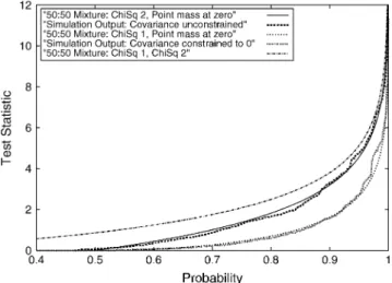
Simulation A:The agreement between the expected
asymptotic and simulation-based empirical distribu-tions when fitting the RR model to data simulated to fit the repeatability model (no change in variance over time and correlation between effects at different ages equal to one) was excellent. The two statistics of inter-est,SDrep1andSDrep2, are expected to follow12x21:120 and 1
2x 2
2:120 distributions, respectively. They are shown in
Figure 1. For comparison the 1 2x
2 2:12x
2
1 distribution is
shown; this shows that neither SDrep1 nor SDrep2
con-verges to this mixture (as suggested in Stramand Lee
1994 and Meyer1998). Note that although the
covari-ance is not constrained to 0 inSDrep2the overall
coef-ficient matrix (C) is constrained to be positive definite.
Simulation B: Deviations from repeatability model: The
power in each case is given in Table 3.SDrep2was more
powerful than SDrep1 at detecting deviations from the
repeatability model. Reducing the relative amount of temporary environment (ratio of permanent to envi-ronmental variance was 75:25 instead of 50:50) resulted in the change in genetic variance over time being easier to detect.
Power to detect QTL: RR, Re, and univariate models:The power to detect a simulated QTL was determined using three statistics, Suni, Srep, and SRR1. The power
(pro-portion of 200 replicates, expressed as a percentage) at different significance levels for variance sets B1, B2, and B3 is given in Tables 4, 5, and 6, respectively.
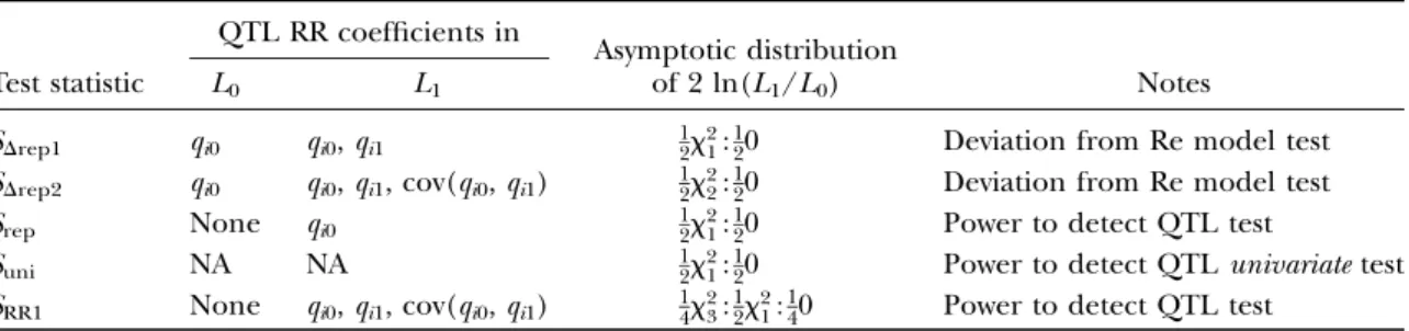
TABLE 2
Summary of statistics, simulations A and B
QTL RR coefficients in
Asymptotic distribution of 2 ln(L1/L0)
Test statistic L0 L1 Notes
SDrep1 qi0 qi0,qi1 12x 2
1:120 Deviation from Re model test SDrep2 qi0 qi0,qi1, cov(qi0,qi1) 12x
2 2:
1
20 Deviation from Re model test
Srep None qi0 12x
2
1:120 Power to detect QTL test
Suni NA NA 1
2x 2
1:120 Power to detect QTLunivariatetest SRR1 None qi0,qi1, cov(qi0,qi1) 14x
2 3:
1 2x
2 1:
1
Looking at the results fromSrepin Tables 4 and 6 we
see that much of the power in the repeatability analysis lies in the reduction in temporary environmental noise as a result of averaging over a number of measures; when the temporary environmental effects are small the repeatability analysis has little power to detect QTL. In contrast, the model allowing for a change in QTL effect over time (SRR1) gains power when the temporary
en-vironmental noise is reduced. This is because the change in genetic variance over time can be more readily de-tected, increasing the power to detect the QTL when a parameter modeling the change in QTL effect over time is fitted. Note also that a modest increase in the genetic variance at age five (compare the results when QTL variance is 0.33 with when it is 0.4, see Tables 4 and 5) has a relatively large effect upon the power whenSRR1is
used; the power to detect the QTL with a LOD of 3 (as-ymptotic significance level 104) rises from 43 to 78%.
Since the five trait values at the five time points have correlation.0 but,1, the uncorrectedSuniis
anticon-servative while theSuni(b)is too conservative. Assuming
that the true power value at the specified significance levels can be obtained by taking a power estimate be-tweenSuniandSuni(b)we see that the repeatability and
univariate methods have similar power.
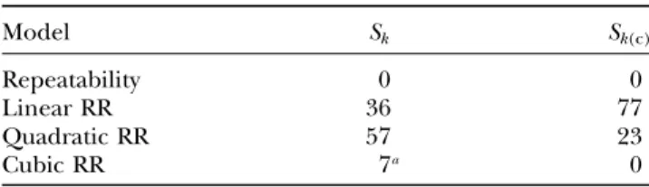
Simulation C1: The procedure outlined above was
used to determine the best-fitting model for the data. Seventy-nine percent of replicates rejected, at the 1% sig-nificance level, the no-QTL model when the Re model was fitted. However, in all cases (200 replicates) the Re model was rejected in favor of the first-degree RR model (All P-values ,105 for S
Drep1 and SDrep2). This was
unsurprising since the data were simulated so that the QTL variance changed over time and the genetic (QTL) correlations were ,1. Sixty-four percent of replicates rejected the linear RR in favor of the quadratic RR when Skwas used to compare the two models. WhenSk(c)was
used only 23% of replicates provided evidence for the quadratic model. UsingSk(c)for the test for a cubic RR
compared with the quadratic fit (for replicates where the quadratic coefficient was significant) resulted in none of the replicates indicating that the cubic fit was better. Assessing the higher-degree models (unconstrained cubic model and quartic model) proved difficult computa-tionally, with many replicates failing to converge to a like-lihood maximum. In the cubic case, roughly one-third of replicates failed to converge (using a maximum of 100 iterations in ASREML) when the unconstrained cubic model (i.e.,Skwas calculated) was fitted. Taking
the likelihoods as calculated (i.e., one-third of them are underestimates of the true likelihood maximum, bi-asing the test statistic for the significance of the cubic term downward), 7% of replicates rejected the qua-dratic model in favor of the cubic model. Only in 35% of
Figure1.—Simulation A results. Fit of the statisticsS Drep1 andSDrep2(for data simulated under the repeatability model) to the expected asymptotic null distributions is shown.
TABLE 3
Simulation B: power to reject the repeatability model in favor of first-degree RR
SDrep1(%) SDrep2(%)
B1 5 41
B2 12 76
B3 16 75
Significance level set to 0.01.
TABLE 4
Simulation B1: power to detect QTL
Significance level
Statistic 103 104 105
Srep(Re QTLvs. no QTL) 54 30 17
Suni(univariate QTLvs. no QTL) 61 33 18 Suni(b)(Bonferroni-correctedSuni) 38 21 9 SRR1(linear RR QTLvs. no QTL) 64 43 31
Data are simulated under simulation model B with QTL var-iance 0.2 (age 1) to 0.33 (age 5) (0.5 permanent environmen-tal variance, 0.5 temporary environmenenvironmen-tal variance).
TABLE 5
Simulation B2: power to detect QTL
Significance level
Statistic 103 104 105
Srep(Re QTLvs. no QTL) 67 41 21
Suni(univariate QTLvs. no QTL) 75 47 24 Suni(b)(Bonferroni-correctedSuni) 53 28 13 SRR1(linear RR QTLvs. no QTL) 85 78 65
Data are simulated under simulation model B with QTL var-iance 0.2 (age 1) to 0.4 (age 5) (0.5 permanent environmental variance, 0.5 temporary environmental variance).
cases could the full multivariate model be maximized. These results are summarized in Table 7.
For a few of the replicates all models could be maximized and a graphic representation of the results of one replicate is given in Figure 2. The variance terms from the QTL RR are expressed as a proportion of the total variance (i.e., QTL heritability). For comparison, the univariate and repeatability model results are su-perimposed on the same graph. This shows that the repeatability model is a poor fit to the simulated model and that the univariate results, while following the simulated model to some degree, are rather noisy. All of the polynomial-based RRs follow the simulated model well; the first-degree model offers an excellent fit with only two extra parameters fitted compared with the re-peatability model. The fourth-degree polynomial fol-lows the univariate results more closely but in this case such variations from the simulated model are simply random variation.
It is instructive to compare the results from simu-lations B and C. In simulation B2, when s2
time1¼0:2; s2
time5¼0:4;SDrep1 rejected the repeatability model in
12% of cases (significance level 1%). In comparison, when the data were simulated in simulation C1 with the same parameters apart from a change in the correlation structure, 100% of replicates rejected the repeatability model (significance level 1%, although in fact all re-jected it at significance level 0.001%). The univariate results for simulation C1 were similar (data not shown) to those obtained for the repeatability analysis (which is
equivalent to an ‘‘average across all measures’’ univari-ate analysis when there is regular age spacing) and were hence substantially less powerful than those obtained from the RR model.
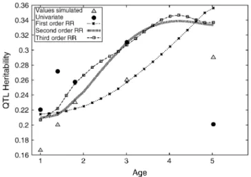
Simulation C2: In simulation C2 71% of replicates
rejected (significance level 1%) the no-QTL model when the Re model was fitted. In all cases (200 rep-licates) the Re model was rejected in favor of the first-degree RR model (all P-values ,106 for S
Drep1 and
SDrep2). Eighty-four percent of replicates rejected the
linear RR in favor of the quadratic RR whenSkwas used
to compare the two models. When the Sk(c)was used
89% of replicates provided evidence for the quadratic model. Note that although the likelihood ratio ofSk(c)is
lower than that ofSk, since the null distributions differ
Sk(c)can sometimes give smallerP-values. UsingSk(c)for
the test for a cubic RR compared with the quadratic fit resulted in 4% of the replicates indicating that the cubic fit was better. This may be a slight underestimate as 5% of the replicates failed to converge to a likelihood maxi-mum. Using the unconstrained cubic model in the test resulted in 17% of replicates rejecting the quadratic model although almost a third failed to converge fully. The quartic and full multivariate models could not be reliably fitted to these data. These results are summa-rized in Table 8. Although simulation C2 showed that polynomial-based CFs worked well with the simulated logarithmic increase in QTL variance with age, non-monotonic changes in QTL variance with age were not considered here (e.g., an increase in genetic effect at earlier ages, followed by a decline in later life).
The results of one replicate are given in Figure 3. The values specified in the simulation model are super-imposed on the graph. As expected, when the change in QTL variance is nonlinear the second- and higher-degree RRs have more utility than the first-higher-degree model. Nonetheless, even the first-degree RR is substantially better than the repeatability model. Once again the univariate results are rather noisy; univariate methods TABLE 6
Simulation B3: power to detect QTL
Significance level
Statistic 103 104 105
Srep(Re QTLvs. no QTL) 30 13 5
Suni(univariate QTLvs. no QTL) 39 18 6 Suni(b)(Bonferroni-correctedSuni) 24 8 4 SRR1(linear RR QTLvs. no QTL) 75 64 46
Data are simulated under simulation model B with QTL var-iance 0.2 (age 1) to 0.33 (age 5) (0.75 permanent environ-mental variance, 0.25 temporary environenviron-mental variance).
TABLE 7
Simulation C1 [QTL variance 0.2 (age 1) to 0.4 (age 5)]: best-fitting model (%)
Model Sk Sk(c)
Repeatability 0 0
Linear RR 36 77
Quadratic RR 57 23
Cubic RR 7a 0
a
One-third of replicates failed to converge so this may be an underestimate.
do not utilize the natural ordering in time of the genetic effects with adjacent measures often yielding very dif-ferent estimates of QTL heritability.
DISCUSSION
This article has described methods suitable for QTL analysis in complex pedigrees of data sets with longitu-dinal trait measures. The multivariate techniques re-quired to effectively analyze such data are more involved than those for single-trait measures. This, together with the relative paucity of suitable data, goes some way to-ward explaining the lack of research in this area. Longi-tudinal traits are often not well described by single, cross-sectional, phenotypic measures but, as has been described, the conceptually simple full multivariate model requires the estimation of large numbers of parameters when there are more than a few time points. Since the data sets commonly available for genetic studies in hu-man or natural populations are small, the full multivar-iate approach has somewhat limited application. Some longitudinal traits will be relatively highly correlated across multiple measures of the same trait compared with nonlongitudinal multivariate measures (e.g., mul-tivariate analysis of height and weight, say). The
sim-ulations performed here showed that when traits are highly correlated the estimation of large numbers of parameters is difficult. The covariance function-based approach may have considerably more utility than the full multivariate model as it can reduce the number of parameters in the model. Fitting a polynomial with de-gree plus one equal to the number of age points in the data is equivalent to a full multivariate model. Fitting lower-degree polynomials smoothes the estimated co-variance function, removing individual deviations that are likely to be due to stochastic variation.
The covariance function approach will be particularly useful when the data are measured at a large number of ages, perhaps with irregular gaps between measures; this is because the approach fits a polynomial through the set of ages available for each individual. Furthermore, individuals measured only for a few ages can still con-tribute to the analysis by providing information on the coefficients of the lower-degree polynomials (informa-tion available on constant and linear terms when there are two age measures and so on). Once the covariance function has been estimated for a given data set, predic-tions of future observapredic-tions can be made using best linear unbiased prediction (e.g., Lynch and Walsh
1998; Mrode1996). For example, predictions could be
made about the trait value of an individual at age 60 given their measurements until age 40 or about the trait value at a particular age for children given the measures taken on their parents.
In simulation B it was shown that when there was a moderate increase in QTL variance over time fitting a first degree RR increased the power to detect the QTL. This increase in power came solely from the RR model-ing the change in QTL variance. The increased effi-ciency of the RR in modeling any decreases in the genetic correlation between trait measures ,1 was ig-nored by simulating data with no decline in genetic correlation with time. The increase in power was partic-ularly large when the ratio of permanent to temporary environment was high (i.e., when most of the environ-mental ‘‘noise’’ affects all of an individual’s trait measures).
At Genetic Analysis Workshop 13 (GAW13) (Almasy et al.2003) reference is made to genes that change their variance over time as slope genes (Gauderman et al.
2003; Geeet al.2003; Raoet al.2003; Yanget al.2003).
The data generated under simulation model B allow a direct test for these slope genes. QTL effects, however, may not be completely correlated across ages and a more realistic simulation model (i.e., simulation model C) will allow the correlations between QTL effects at dif-ferent ages to decrease.
It is not possible to know what form real-life genetic CFs take. It was assumed in simulation C that the decline in correlation followed a steady decrease with increasing time separation (i.e., we intentionally did not simulate data under the polynomial-based analysis method used TABLE 8
Simulation C2 [QTL variance 0.2 (age 1) to 0.4 (age 5)]: best-fitting model (%)
Model Sk Sk(c)
Repeatability 0 0
Linear RR 16 11
Quadratic RR 67 85
Cubic RR 17a 4b
a
Almost one-third of replicates failed to converge so this may be an underestimate.
b
Five percent of replicates failed to converge so this may be a slight underestimate.
Figure3.—Sample results, Simulation C2.
for the CF-based analyses; polynomials do not generate correlation structures of the ‘‘banded’’ type used in si-mulation C). The correlation was assumed to remain relatively high over the range of ages of interest. This seems likely to be true for QTL effects (whose constit-uent element is one or more closely linked genes) but may be less likely to hold for polygenic effects (whose constituent elements are more heterogeneous and will change over life). The shape of possible CFs for poly-genic effects has been considered by Jaffrezic and
Pletcher(2000); the models considered ranged from
one in which the correlation structure remained high across ages to another in which the correlation became negative at widely separated ages. They concluded that polynomial-based CFs were most effective when the correlation remained high over widely separated ages
( Jaffrezicand Pletcher2000).
The model selection (choice of polynomial fit) in simulation C was based on differences in likelihood. To ensure parsimony and robustness, we advise utilization of low-degree polynomials. Although high-degree poly-nomials may provide a good fit to the data, if the method is to be used for QTL detection then the benefits of improved fit may be outweighed by the increase in the degrees of freedom. It is also important to note that with most realistic sample sizes it is not possible to fit high-degree polynomials and the problem of model selection may be of little practical consequence. For genome scan-ning we recommend application of the Re model (zero-degree RR), the first-(zero-degree RR model, and, where data permit (large sample size), the second-degree RR model. The testing of multiple polynomial fits increases the computational load and also the number of tests done. Note that the requirement for multiple tests in QTL analysis is not new here; many QTL mapping methods for line crosses apply multiple models at each location across the genome (e.g., additive model and additive plus dominance model). If computational time is a limiting factor, scanning could be performed with moderate intermarker spacing with first-degree poly-nomials with regions achieving nominal significance (P,0.05) followed up by spacing at 1-cM intervals with second-degree polynomials (or a higher degree if suf-ficient data are available). When we applied the RR methodology to a real data set [the Framingham Heart Study data set from GAW13 (Almasy et al.2003)] we
were not able to fit a second-degree RR (first-degree RRs were fine) to every position across the chromosomes we examined (Macgregoret al. 2003). For simplicity we
used two-generation families (parents and offspring had phenotypes and genotypes) with a single linked marker in our simulations. An illustration of the application of the RR methodology to three-generation extended fam-ilies and genome scan data are given in our GAW13 article (Macgregoret al.2003). Note that since the IBD
computation and phenotype modeling steps are sepa-rate in our analysis the practical application of our
method is identical for single-marker or multiple-marker (multipoint) data.
Although fitting a model that estimates the full set of (co)variances in the data [there arew(w11)/2 to esti-mate when there arewtrait measures] can capture the change in QTL variance over time, such methods are inefficient in most cases and are difficult to apply in practice. One of the primary aims of this article was to investigate how much information can be extracted from longitudinal data in realistic scenarios. The work here and other work on human data sets (deAndrade et al.2002; deAndrade and Olswold2003) indicate
that approaches that do not simplify the covariance structure are unworkable in practice (the relatively small data sets do not support the estimation of large numbers of parameters). In an application of the full multivariate model to trivariate human genetic data (de
Andradeet al.2002;deAndradeand Olswold2003)
the six parameters (three variances, three covariances) could not be estimated simultaneously for all of the random effects. When the situation was approximated by three bivariate analyses, parameter estimation was possible. Given that the trivariate data in these articles
(deAndrade et al.2002; de Andrade and Olswold
2003) support the estimation of only three parameters it would probably be better to fit a first-degree RR to the full set of three traits than to fit three separate full mul-tivariate analyses to three different subsets of the data.
To allow comparison between the different methods, asymptotic results were utilized. In the case where the first-degree RR was compared with the Re model, the asymptotic result was validated by simulation (Figure 1). For the test of first-degree RR QTL vs. no QTL the asymptotic result used (1
4x 2 3:12x
2
1:140) is the same as that
used in a bivariate VC analysis by Amoset al.(2001); we
note that there is disagreement in the literature on this matter, with the described asymptotic distribution from Wang(2003) appearing to disagree with the
distribu-tion described by Amos et al. (2001). We performed
simulations under a no-QTL model (with constant polygenic heritability of 0.20) and found results consis-tent with those described in Amoset al.(2001) (data not
shown). We also note that it is important to simulate either a polygenic or a QTL effect (or both) to evaluate the null distribution; in the univariate case the null distribution when neither effect is simulated appears to be1
4x 2
1:340 (cf.the usual12x 2
1:120 in the univariate QTL test)
when a QTL plus polygenic model is compared with a polygenic model. If the distribution of the traits is not multivariate normal the asymptotic distribution may not be appropriate (incorrect type I error). In such cases gene-dropping simulations can be used to evaluate an empirical null distribution for the test of the overall significance of a QTL. Such simulations use the data structure from the actual data and generate replicates with a marker unlinked to the QTL. Although this ap-proach requires a relatively large number of replicates for smallP-values this procedure needs to be done only once per genome scan and can typically be completed in
,1 day with current computing power. Instead of simply comparing the observed test statistic with the relevant percentile of the empirical distribution, the number of replicates required can be reduced either by fitting a parametric distribution to the empirical distribution
(Dudbridgeand Koeleman2004) or by performing a
regression of the empirical distribution on the expected asymptotic distribution. This latter approach allows the rescaling of the results so that the asymptotic distribu-tion is valid and is implemented in the program SOLAR for univariate analysis (Almasyand Blangero1998).
Genomewide significance can be dealt with when using the methods we describe here. For human data the P-value required for genomewide significance is generally assumed to be in the range 0.0001–0.00005
(Landerand Kruglyak1995). Suggestive significance
requires P-values ,0.002. Since a number of models may be fitted per genomic location we recommend using slightly more stringent thresholds than those given in Lander and Kruglyak (1995); thresholds
twofold lower than the Lander and Kruglyak levels would seem reasonable (given that no more than a few models will be utilized and they are unlikely to be uncorrelated). The P-value obtained from either the asymptotic results or gene-dropping simulations (see above) can be compared with the threshold values and
significance (suggestive, genomewide) declared accord-ingly. For other species the relevant thresholds can be determined by taking into account the species’ genome length.
One disadvantage of the RR techniques is that the method specifies the correlation structure and change in variance (over time) together. A low-degree poly-nomial may be adequate to model the change in vari-ance over time but inadequate for approximating the covariance structure or vice versa. Alternative models that fit separate functions for the change in variance and the change in correlation or covariance have been proposed for polygenic effects (character process
mod-els,e.g., Pletcherand Geyer1999; Diegoet al.2003).
Alternative techniques for longitudinal QTL map-ping in structured populations have been developed recently (Maet al.2002; Wuet al.2004a). Such mapping
techniques assume that the QTL is a fixed effect with a specified number of alleles and this allows for sophisti-cated modeling of the change in QTL effect over time (Maet al.2002; Wuet al.2004a). The application of such
fixed-effect models has led to a greater understanding of the genetic architecture of growth in organisms such as mice and forest trees (Wuet al.2004a,b). In contrast
to this, the methodology described here is based upon random-effects modeling, where we assume that the distribution of QTL effects is normal. This allows us to circumvent the estimation of QTL allele frequencies and facilitates ready application of our method to arbi-trary pedigrees. Given the matrix of QTL-specific IBD probabilities [estimated from the marker data (Almasy
and Blangero1998; Georgeet al.2000)] our method
can be applied without modification to a wide variety of family structures. Further discussion of the differences between fixed- and random-effect QTL models is given
in Georgeet al.(2000).
A number of other methods for allowing analyses of multivariate data have been proposed. In most cases these are for distinct multiple traits (height, weight, etc.) rather than for longitudinal ones (height at age 20, at age 30,. . .). The simplest approach involves perform-ing separate univariate analyses for each trait. This ap-proach does not take advantage of the potential power gains inherent in the multivariate structure of the data. Furthermore, it is unclear how to keep the significance level at the desired level when there are multiple tests. A Bonferroni correction can be readily applied but this is almost certain to be overly conservative. The simula-tions performed here showed that univariate methods offered similar power to repeated measures methods and were often hence substantially less powerful than RR-based approaches. The next simplest alternative is to transform the multiple-trait values into a single sum-mary or composite measure, thus allowing a single univariate analysis method to be used. This composite measure can be constructed such that the calculated ‘‘factor score’’ maximizes some parameter of interest,
such as the heritability (Boomsma and Dolan 1998).
Furthermore, a multivariate segregation analysis has been proposed for pedigree data (Blangero and
Konigsberg1991) and this may allow the construction
of a composite measure that is particularly suitable for mapping the major gene affecting a trait. However, even in this second case where there may be more power to detect a particular QTL or locus, neither method is likely to give an optimal composite measure for other QTL or loci (Eaveset al.1996).
A number of authors have considered extensions of the sib-pair regression methods to multivariate data (Amoset al.1990; Allisonet al.1998;deAndradeand
Olswold 2003; Huang and Jiang 2003; Mirea et al.
2003). Such methods offer advantages over the VC-based multivariate approaches in terms of computational ease but, in addition to their unsuitability for extended fami-lies, they have been shown to offer less power than VC-based approaches (for bivariate data see Amoset al.2001).
Multivariate linkage analysis related to that described
inmaterials and methodshas been described for
sib-pair data (Eaveset al.1996) and livestock and
experi-mental cross data ( Jiangand Zeng1995; Knottand
Haley 2000; Sorensen et al. 2003) and applied to
developmental dyslexia data in sib pairs (Marlowet al.
2003). The method used by Marlowet al.(2003) fitted
the polygenic effect as in Equation 3 but the covariance structure of the random effect for the QTL was con-strained such that correlation between any two trait measures was equal to one. This means that there are only kparameters to estimate when there are k traits [compared withk(k11)/2 with an unstructured QTL covariance matrix]. While this is unlikely to be true for all but the most strongly related traits, this model may allow parameter estimation in cases in which there are limited amounts of data.
In this study we have extended the RR approach to allow QTL analysis of longitudinal data. The methods described appropriately take into account the ordering in trait values over time. Computer simulations have shown that the RR-based approach offers consider-able increases in power compared with univariate and repeatability-based techniques. It should be possible to take advantage of this extra power by fitting first-degree random regressions to most realistic human/natural population data sets.
We thank Robin Thompson for providing advice on the program ASREML. We thank the anonymous referees for helpful comments on a previous version of this manuscript. We gratefully acknowledge financial support from the following organizations: Akzo-Nobel (Organon), the Biotechnology and Biological Sciences Research Council, the Royal Society, and the Higher Education Funding Council for Wales.
LITERATURE CITED
Allison, D. B., B. Thiel, P. St. Jean, R. C. Elston, M. C. Infante
et al., 1998 Multiple phenotype modeling in gene-mapping
studies of quantitative traits: power advantages. Am. J. Hum. Genet.63:1190–1201.
Almasy, L., and J. Blangero, 1998 Multipoint quantitative-trait
linkage analysis in general pedigrees. Am. J. Hum. Genet.62:
1198–1211.
Almasy, L., L. A. Cupples, E. W. Daw, D. Levy, D. Thomaset al.,
2003 Genetic analysis workshop 13: introduction to workshop summaries. Genet. Epidemiol.25:S1–S4.
Amos, C. I., 1994 Robust variance-components approach for
assess-ing genetic linkage in pedigrees. Am. J. Hum. Genet.54:535– 543.
Amos, C. I., R. C. Elston, G. E. Bonney, B. J. B. Keatsand G. S.
Berenson, 1990 A multivariate method for detecting
genetic-linkage, with application to a pedigree with an adverse lipopro-tein phenotype. Am. J. Hum. Genet.47:247–254.
Amos, C. I., M.deAndradeand D. K. Zhu, 2001 Comparison of
multivariate tests for genetic linkage. Hum. Hered.51:133–144. Blangero, J., and L. W. Konigsberg, 1991 Multivariate segregation
analysis using the mixed model. Genet. Epidemiol.8:299–316. Boomsma, D. I., and C. V. Dolan, 1998 A comparison of power to
detect a QTL in sib-pair data using multivariate phenotypes, mean phenotypes, and factor scores. Behav. Genet.28:329–340.
deAndrade, M., and C. Olswold, 2003 Comparison of
longitudi-nal variance components and regression based approaches for linkage detection on chromosome 17 for systolic blood pressure. BMC Genet.4:S17.
deAndrade, M., R. Gueguen, S. Visvikis, C. Sass, G. Siestet al.,
2002 Extension of variance components approach to incorpo-rate temporal trends and longitudinal pedigree data analysis. Genet. Epidemiol.22:221–232.
Diego, V. P., L. Almasy, T. D. Dyer, J. M. P. Solerand J. Blangero,
2003 Strategy and model building in the fourth dimension: a null model for genotype (x) age interaction as a gaussian station-ary stochastic process. BMC Genet.4:S34.
Dudbridge, F., and B. P. C. Koeleman, 2004 Efficient computation
of significance levels for multiple associations in large studies of correlated data, including genomewide association studies. Am. J. Hum. Genet.75:424–435.
Eaves, L. J., M. C. Nealeand H. Maes, 1996 Multivariate multipoint
linkage analysis of quantitative trait loci. Behav. Genet.26:519– 525.
Gauderman, W. J., S. Macgregor, L. Briollais, K. Scurrah,
M. Tobinet al., 2003 Longitudinal data analysis in pedigree
studies. Genet. Epidemiol.25:S18–S28.
Gee, C., J. L. Morrison, D. C. Thomasand W. J. Gauderman,
2003 Segregation and linkage analysis for longitudinal meas-urements of a quantitative trait. BMC Genet.4:S21.
George, A. W., P. M. Visscherand C. S. Haley, 2000 Mapping
quantitative trait loci in complex pedigrees: a two-step variance component approach. Genetics156:2081–2092.
Gilmour, A. R., B. J. Gogel, B. R. Cullis, S. J. Welham and
R. Thompson, 2002 ASREML User Guide Release 1.0.VSN
Inter-national, Hemel Hempstead, UK.
Goldgar, D. E., 1990 Multipoint analysis of human quantitative
genetic-variation. Am. J. Hum. Genet.47:957–967.
Haseman, J. K., and R. C. Elston, 1972 The investigation of linkage
between a quantitative trait and a marker locus. Behav. Genet.1:
11–19.
Hoeschele, I., P. Uimari, F. E. Grignola, Q. Zhangand K. M. Gage,
1997 Advances in statistical methods to map quantitative trait loci in outbred populations. Genetics147:1445–1457. Hopper, J. L., and J. D. Mathews, 1982 Extensions to multivariate
normal-models for pedigree analysis. Ann. Hum. Genet.46:373– 383.
Huang, J. A., and Y. M. Jiang, 2003 Genetic linkage analysis of a
dichotomous trait incorporating a tightly linked quantitative trait in affected sib pairs. Am. J. Hum. Genet.72:949–960. Jaffrezic, F., and S. D. Pletcher, 2000 Statistical models for
esti-mating the genetic basis of repeated measures and other function-valued traits. Genetics156:913–922.
Jamrozik, J., L. R. Schaefferand J. C. M. Dekkers, 1997 Genetic
evaluation of dairy cattle using test day yields and random regres-sion model. J. Dairy Sci.80:1217–1226.
Jiang, C. J., and Z. B. Zeng, 1995 Multiple-trait analysis of
Kirkpatrick, M., D. Lofsvoldand M. Bulmer, 1990 Analysis of the
inheritance, selection and evolution of growth trajectories. Genetics124:979–993.
Knott, S. A., and C. S. Haley, 2000 Multitrait least squares for
quantitative trait loci detection. Genetics156:899–911. Lander, E., and L. Kruglyak, 1995 Genetic dissection of complex
traits—guidelines for interpreting and reporting linkage results. Nat. Genet.11:241–247.
Lange, K., J. Westlakeand M. A. Spence, 1976 Extensions to
ped-igree analysis. III. Variance components by the scoring method. Ann. Hum. Genet.39:485–491.
Lynch, M., and B. Walsh, 1998 Genetics and Analysis of Quantitative
Traits.Sinauer Associates, Sunderland, MA.
Ma, C. X., G. Casellaand R. L. Wu, 2002 Functional mapping of
quantitative trait loci underlying the character process: a theoret-ical framework. Genetics161:1751–1762.
Macgregor, S., 2003 Genetic linkage analysis in complex
pedi-grees. Ph.D. Thesis, University of Edinburgh, Edinburgh. Macgregor, S., S. A. Knott, I. Whiteand P. M. Visscher, 2003
Lon-gitudinal variance-components analysis of the Framingham heart study data. BMC Genet.4:S22.
Marlow, A. J., S. E. Fisher, C. Francks, I. L. MacPhie, S. S. Cherny
et al., 2003 Use of multivariate linkage analysis for dissection of a complex cognitive trait. Am. J. Hum. Genet.72:561–570. Meyer, K., 1998 Estimating covariance functions for longitudinal
data using a random regression model. Genet. Sel. Evol.30:
221–240.
Mirea, L., S. B. Bull and J. Stafford, 2003 Comparison of
haseman-elston regression analyses using single, summary, and longitudinal measures of systolic blood pressure. BMC Genet.
4:S23.
Mrode, R. A., 1996 Linear Models for the Prediction of Animal Breeding
Values.CAB International, Wallingford, UK.
Pletcher, S. D., and C. J. Geyer, 1999 The genetic analysis of
age-dependent traits: modeling the character process. Genetics153:
825–835.
Rao, S. Q., L. Li, X. Li, K. L. Moser, Z. Guoet al., 2003 Genetic
link-age analysis of longitudinal hypertension phenotypes using three summary measures. BMC Genet.4:S24.
Self, S. G., and K. Y. Liang, 1987 Asymptotic properties of
maximum-likelihood estimators and likelihood ratio tests under nonstandard conditions. J. Am. Stat. Assoc.82:605–610. Sorensen, P., M. S. Lund, B. Guldbrandtsen, J. Jensen and
D. Sorensen, 2003 A comparison of bivariate and univariate
qtl mapping in livestock populations. Genet. Sel. Evol.35:605–622. Stram, D. O., and J. W. Lee, 1994 Variance-components testing in
the longitudinal mixed effects model. Biometrics50:1171–1177 [erratum: Biometrics51:1196 (1995)].
Wang, K., 2003 Mapping quantitative trait loci using multiple
phe-notypes in general pedigrees. Hum. Hered.55:1–15.
Wu, R. L., C. X. Ma, M. Linand G. Casella, 2004a A general
frame-work for analyzing the genetic architecture of developmental characteristics. Genetics166:1541–1551.
Wu, R. L., Z. H. Wang, W. Zhaoand J. M. Cheverud, 2004b A
mechanistic model for genetic machinery of ontogenetic growth. Genetics168:2383–2394.
Yang, Q., I. Chazaro, J. Cui, C. Y. Guo, S. Demissie et al.,
2003 Genetic analyses of longitudinal phenotype data: a com-parison of univariate methods and a multivariate approach. BMC Genet.4:S29.
Communicating editor: J. B. Walsh