ABSTRACT
VAZIRI ASTANEH, ALI. On the Forward and Inverse Computational Wave Propagation Problems. (Under the direction of Dr. Murthy N. Guddati.)
This dissertation provides efficient algorithms for forward and inverse modeling of wave propagation problems. The presented methods are verified with synthetic examples and validated with real-life experiments in near surface imaging and nondestructive testing applications.
First, we study the dispersion analysis of guided waves in the layered waveguides and half-spaces which involves solution of eigenvalue problems. This mathematical model is often used in applications such as near surface imaging, pavement structures characterization and thickness gauging of pipelines. We apply the new discretization technique termed Complex-Length Finite Element Method (CFEM) which increases the efficiency of forward modeling for such piecewise homogenous media, thus reducing the computational cost of associated inverse problems that rely on multiple forward solves.
Second, we consider the near surface imaging problem and propose an approximate analytical gradient that facilitates more efficient inversion using surface waves. We show that the improvements in both venues, i.e. forward modeling and inversion scheme, leads to an order-of-magnitude reduction in computational cost.
Third, we focus on efficient simulation of immersed waveguides and propose the use of Perfectly Matched Discrete Layer (PMDL) for modeling the surrounding fluid. Immersed plates, fluid-filled pipes and immersed waveguides with arbitrary cross-section are considered and the guidelines for choosing the discretization parameters are provided. Numerical examples demonstrate the increased efficacy in obtaining the dispersion characteristics.
On the Forward and Inverse Computational Wave Propagation Problems
by
Ali Vaziri Astaneh
A dissertation submitted to the Graduate Faculty of North Carolina State University
in partial fulfillment of the requirements for the degree of
Doctor of Philosophy
Civil Engineering
Raleigh, North Carolina 2016
APPROVED BY:
_______________________________ ________________________________ Dr. Murthy N. Guddati Dr. Shamimur Rahman
Committee Chair
DEDICATION
BIOGRAPHY
ACKNOWLEDGMENTS
I am delighted to express my gratitude to my advisor, Dr. Murthy Guddati, for guiding me through the multitude of challenges in my research. I certainly will miss the brainstorming and creative discussions with him.
I would like to thank Dr. Shamimur Rahman, Dr. Kazufumi Ito and Dr. Wilkins Aquino for serving as members of the advisoral committee
Also many thanks to my friends: Dr. Alireza Sadeghirad, Dr. Mehran Eslaminia, Dr. Senganal Thirunavukkarasu, Dr. Arash Dehghan Banadaki and Dr. Siddharth Savadatti.
TABLE OF CONTENTS
LIST OF TABLES ... ix
LIST OF FIGURES ... x
Chapter 1 ... 1
1.1 Exponentially convergent linear finite elements... 1
1.2 Dispersion analysis of embedded waveguides ... 2
1.3 Near-surface imaging ... 2
1.4 Dispersion analysis of immersed waveguides ... 3
1.5 Domain decomposition for Helmholtz problem ... 4
Chapter 2 ... 1
2.1 Introduction ... 1
2.2 Preliminaries ... 4
2.2.1 Problem statement ... 4
2.2.2 Dimensional reduction ... 5
2.2.3 A closer look at the DtN map ... 6
2.3 Complex-length finite element method (CFEM) ... 9
2.3.1 Linear finite elements with midpoint integration ... 9
2.3.2 An alternative view: first-order form ... 10
2.3.3 Selection of the mesh parameters ... 12
2.3.4 Summary: CFEM discretization procedure and additional properties ... 16
2.4 CFEM for vector equations (elastodynamics) ... 19
2.4.1 Model Problem... 19
2.4.2 Impedance-preserving property and propagation factor of the mid-point integrated element ... 21
2.5 Numerical examples and discussion ... 23
2.5.1 Two-point boundary value problem: elliptic equation... 23
2.5.2 Two-point boundary value problem: Helmholtz equation ... 24
2.5.3 Comparison with spectral FEM ... 29
2.5.4 Two-dimensional layer: Laplace equation ... 29
2.5.6 Two-dimensional Helmholtz problem with multiple subdomains... 31
2.5.7 Two-dimensional elastodynamics problem with multiple subdomains ... 32
Chapter 3 ... 34
3.1 Introduction ... 34
3.2 Overview of the proposed algorithms ... 36
3.3 Preliminaries: numerical solution of multilayered elastic media ... 37
3.3.1 Model problem ... 37
3.3.2 Finite element approach ... 39
3.4 Complex-length finite element method for discretizing finite layers ... 42
3.4.1 Vertical Dispersion Relation ... 43
3.4.2 Properties of midpoint integrated linear finite elements ... 44
3.4.3 CFEM construction ... 47
3.5 Treatment of half-spaces using Perfectly Matched Discrete Layers ... 51
3.6 Numerical examples... 54
3.6.1 Performance of CFEM for obtaining dispersion curves ... 55
3.6.2 Performance of CFEM for obtaining surface displacements ... 59
3.6.3 Performance of PMDL for modeling infinite half-spaces ... 61
3.6.4 Performance of CFEM for obtaining Lamb wave dispersion curves ... 64
Chapter 4 ... 66
4.1 Introduction ... 66
4.2 Preliminaries: multi-station surface wave inversion ... 69
4.2.1 Acquisition and data processing: multimodal and effective dispersion curves 70 4.2.2 Inverse problem formulation and optimization scheme... 72
4.3 Forward problem: computation of dispersion curves ... 73
4.3.1 Efficient forward modeling using complex-length FEM and perfectly matched discrete layers... 75
4.4 Computation of the Jacobian: differentiation of dispersion curves ... 77
4.5 Numerical examples... 82
4.5.1 Synthetic examples ... 82
4.5.2 Real experiment 1: inversion of Lamb waves ... 87
Chapter 5 ... 92
5.1 Introduction ... 92
5.2 Overview ... 94
5.3 Plates Immersed in Fluid ... 96
5.3.1 Governing equations ... 96
5.3.2 Proposed numerical techniques: CFEM and PMDL ... 98
5.3.3 Characteristics of solid-born wavemodes ... 99
5.3.4 Numerical examples... 103
5.4 Immersed rods and (fluid-filled) pipes ... 107
5.4.1 Governing equations ... 107
5.4.2 Radial discretization and choice of parameters ... 108
5.4.3 Numerical examples... 109
5.5 Immersed waveguides with general cross-section ... 112
5.5.1 Governing equations ... 112
5.5.2 Two-dimensional discretization using CFEM, high-order FEM and PMDL . 113 5.5.3 Numerical examples... 114
5.6 Validation ... 118
5.6.1 Immersed plate: hard/soft solid-fluid interface ... 118
5.6.2 Immersed fluid-filled pipe: hard solid-fluid interface ... 119
5.6.3 Immersed rod: hard solid-fluid interface ... 120
Chapter 6 ... 121
6.1 Introduction ... 121
6.2 Domain decomposition methods for the Helmholtz problem ... 124
6.2.1 Model Problem... 124
6.2.2 Single Lagrange multiplier field methods... 125
6.2.3 Two Lagrange multiplier fields methods ... 126
6.2.4 Optimized Schwarz method ... 128
6.2.5 Preconditioning through coarse space augmentation ... 130
6.3 New interface conditions based on perfectly matched discrete layers ... 131
6.3.1 The method of perfectly matched discrete layers ... 132
6.4 New approach for coarse space: using interface waves ... 136
6.5 Numerical examples... 138
6.5.1 Homogeneous waveguide and full space problems ... 138
6.5.2 Heterogeneous subsurface problem ... 145
Chapter 7 ... 148
7.1 Exponentially convergent linear finite elements... 148
7.2 Dispersion analysis of embedded waveguides ... 149
7.3 Near-surface imaging ... 150
7.4 Dispersion analysis of immersed waveguides ... 151
7.5 Domain decomposition for Helmholtz problem ... 152
REFERENCES ... 153
APPENDICES ... 175
Appendix A ... 176
Appendix B ... 178
Appendix C ... 182
Appendix D ... 184
Appendix E ... 187
Appendix F... 189
Appendix G ... 191
LIST OF TABLES
Table 2.1 Element lengths for varying number of elements ( )n . The domain size is unity. For
other cases, the element lengths simply scale with domain size. ... 15
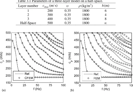
Table 3.1 Parameters of a three-layer model on a half-space. ... 55
Table 3.2 Parameters of a one-layer model on a half-space. ... 61
Table 3.3 Parameters of a four-layer composite plate. ... 65
Table 4.1 Physical parameters of the four-layer synthetic models. ... 83
Table 4.2 Computational cost comparison for synthetic examples. ... 86
Table 4.3 Inversion results for steel plates with the measured thicknesses h11251 mμ and 2 250 1 mμ h . ... 89
Table 4.4 Inversion results for glass plate with the measured thickness h2101 mμ . ... 89
Table 4.5 Computational cost comparison for real experiment 2. ... 91
Table 5.1 Parameters of the tri-laminate immersed plate in motor oil. Complex element lengths for a unit-thickness layer is given in Table 1 of [211]. These vales should be simply multiplied by the actual thickness of each layer. ... 104
Table 5.2 Material properties. ... 104
Table 5.3 Parameters of a tri-laminate immersed plate in motor oil. ... 106
Table 5.4 Parameters of a tri-laminate hard pipe filled with and immersed in motor oil. .... 110
Table 5.5 Parameters of a tri-laminate soft pipe filled with and immersed in motor oil. ... 111
Table 5.6 Parameters of a bi-laminate immersed rod in motor oil. ... 114
Table 5.7 Parameters of a bi-laminate immersed rod in motor oil. ... 116
Table 6.1 Scalability study with respect to mesh size for a fixed number of subdomains 16, 20 and 0 s N n . ... 141
Table 6.2 Strong subdomain scalability study with respect to subdomain numbers for a fixed mesh size h1/ 360,20 and n10 using interface (IW) and plane waves (PW). ... 142
Table 6.3 Strong subdomain scalability study with respect to subdomain numbers for a fixed mesh size h1/ 360,20 and nnoptimal. ... 143
Table 6.4 Weak subdomain scalability study of example 1 with respect to subdomain numbers for a fixed subdomain size H h/ 50,20 and nnoptimal. ... 144
Table 6.5 Scalability study with respect to frequency for a fixed number of subdomains 16, s N hconstant and nnoptimal. ... 145
LIST OF FIGURES
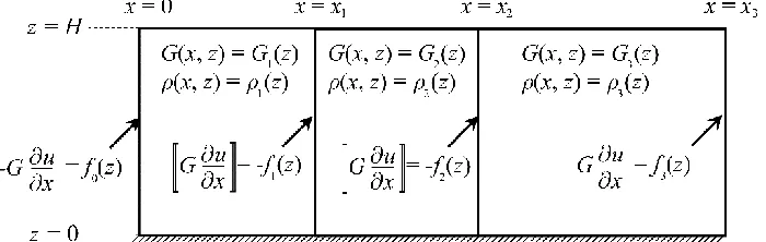
Figure 2.1 A schematic of the model problem. An elastic layer is deforming out of plane under external excitation f0,1,2,3 at the vertical interfaces. The segments bounded by these interfaces can be stratified in the vertical direction. The goal is to obtain the responses at the interfaces. ... 3 Figure 2.2 Finite element meshes for (a) odd number of elements and (b) even number of
elements. ... 16 Figure 2.3 Convergence for the two-point elliptic boundary value problem. The left most curve
corresponds to 10, while the right most curve corresponds to an extremely high decay parameter of 200. ... 24 Figure 2.4 Convergence for the Helmholtz boundary value problem for varying frequencies.
The left most curve in each figure corresponds to the lowest frequency of 4, while the right most curve corresponds to the highest frequency of 40. The meshes shown in Figure 2.2 are used for computation. Note that the error does not converge to a small value for high frequencies, which can be overcome by reordering of elements (cf. Figure 2.6). ... 25 Figure 2.5 Representative meshes after element reordering for (a) 5-element and 10-element
meshes and (b) 15-element and 20-element meshes. Note that the bounds of imaginary part of the nodal coordinates are reducing with refinement. This counters the numerical growth and helps achieve better convergence (compare these meshes with the meshes in Figure 2.2). ... 26 Figure 2.6 Convergence for the two-point Helmholtz boundary value problem after element
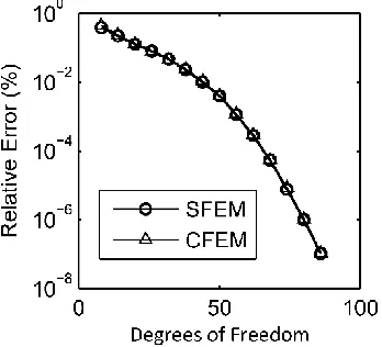
reordering shown in Figure 2.5. In comparison with Figure 2.4, the error is converging to a much smaller value, illustrating the effectiveness of element reordering. ... 27 Figure 2.7 Condition numbers of CFEM (normalized with respect to spectral FEM) for the
Helmholtz problem with 40, (a) without element reordering and (b) with element reordering. ... 28 Figure 2.8 Convergence curves for (a) the two-point elliptic boundary value problem and (b)
the two-point Helmholtz boundary value problem using CFEM and spectral FEM. ... 28 Figure 2.9 Convergence of CFEM for Laplace equation in 2D. Note the exponential
convergence in CFEM discretization as opposed to algebraic convergence of regular FEM (left plot is semi-log and the right plot is log-log). For 1% relative error, one would need 10 CFEM elements as opposed to 100 regular elements. 0.01% relative error requires just 14 CFEM elements, as opposed to 1000 regular finite elements. ... 30 Figure 2.10 Convergence of CFEM for Helmholtz equation in a two-dimensional setting. Note
Figure 2.11 Convergence for multiple-subdomain problem. Note the exponential convergence of CFEM. For 1% relative error, we would need 20 CFEM elements as opposed to 300 regular finite elements. 0.1% error tolerance requires 28 CFEM elements as opposed to more than 800 regular finite elements. ... 32 Figure 2.12 Convergence for multiple-subdomain elastodynamics problem. For 1% relative
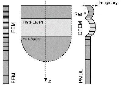
error, we would need 28 CFEM elements as opposed to 500 regular finite elements. 0.1% error tolerance requires 60 CFEM elements as opposed to more than 1000 regular finite elements... 33 Figure 3.1 Overview of the proposed methods: (a) CFEM discretization of finite layers with
complex conjugate depths. The resulting CFEM mesh is bent into complex plane (on the right), but requires considerably less elements in comparison with regular finite element mesh (on the left); (b) PMDL discretization of half-spaces. Typically, 2-4 PMDL elements with drastically graded mesh (on the right) is sufficient to capture the effect of the half-space, compared to much larger number of regular finite elements (on the left). Thus, CFEM and PMDL facilitate accurate simulation of layered waveguides and half-spaces. ... 37 Figure 3.2 Layered waveguide geometry of a composite plate. ... 38 Figure 3.3 (a) Geometry of an elastic layer in a stratified medium and (b) discretized layer with
mid-point integrated finite elements. ... 43 Figure 3.4 (a) Mid-point integrated layer [0, ]L plus the half-space [ , )L and (b) the entire
half-space [0, ) . Impedance preserving property ensures that the impedance of both half-spaces are identical at the top surface. ... 45 Figure 3.5 (a) Bottom homogeneous half-space, (b) complex coordinate stretching, (c)
discretization with mid-point integrated layers and (d) truncation with homogeneous Dirichlet boundary condition. ... 52 Figure 3.6 Phase velocity curves using (a) complex-length FEM and (b) regular FEM with 27
elements. ... 55 Figure 3.7 Relative error in the phase velocity using (a) complex-length FEM and (b) regular
FEM with 27 elements (note that the vertical scales are different). ... 56 Figure 3.8 (a) Phase velocity curves and (b) relative error in phase velocity using regular FEM
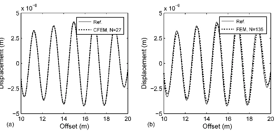
with 90 elements. ... 57 Figure 3.9 Convergence curves of phase velocity using regular and complex-length FEM. . 58 Figure 3.10 Convergence curves of phase velocity using the complex-length and spectral FEM. ... 58 Figure 3.11 Real part of the surface displacement response using (a) complex-length FEM with
27 elements (N 27) and (b) regular FEM with 135 elements (N135) at 100 Hz
f ... 60 Figure 3.12 Imaginary part of the surface displacement response using (a) complex-length
FEM with 27 elements (N 27) and (b) regular FEM with 135 elements (N 135) at f 100 Hz. ... 60 Figure 3.13 Convergence curves of the surface displacement using the complex-length and
Figure 3.14 Phase velocity curves using (a) PMDL method and (b) regular FEM with the graded mesh parameters n4, L11.1 and3. ... 62 Figure 3.15 Relative error in phase velocity using (a) PMDL method and (b) regular FEM with
the graded mesh parameters n4, L11.1 and 3 (note that the vertical scales are different)... 63 Figure 3.16 (a) Relative error in phase velocity using (a) PMDL method with the graded mesh
parameters n6, L1 1,2 and (b) regular FEM with the graded mesh parameters (note that the vertical scales are different). ... 63 Figure 3.17 Phase velocity of Lamb waves using (a) complex-length FEM with 40 elements
and (b) regular FEM with 140 elements (note that the vertical scales are different). ... 64 Figure 4.1 Schematic of multi-station surface wave inversion: (a) experimental setup where
the surface waves are generated and recorded at the surface; (b) surface trace representing the measured response histories; (c) transformed signal in frequency-wavenumber (f-k) domain; (d) dispersion curves obtained by processing the f-k signal; and (e) layer properties estimated through inversion. ... 69 Figure 4.2 Theoretical and effective dispersion curves using (a) 240, (b) 36, and (c) 12 receivers
for the synthetic example (model 3 of Table 4.1). ... 71 Figure 4.3 (a) Layered half-space with a vertical surface load, (b) mathematical model of the
finite depth layers and the bottom infinite layer. ... 73 Figure 4.4 Proposed methods for forward modeling: (a) CFEM discretization of finite layers
with complex conjugate depths. The resulting CFEM mesh is mapped into the complex plane (on the right), but requires much fewer elements in comparison with regular finite element mesh (on the left); (b) PMDL discretization of half-spaces. Typically, 2-5 PMDL elements with drastically graded mesh (on the right) is sufficient to capture the effect of the half-space, compared to much larger number of regular finite elements (on the left). Thus, CFEM and PMDL facilitate accurate simulation of layered waveguides and half-spaces. ... 75 Figure 4.5 Misfit function (and its close-up) as a function of the shear velocity of the first layer. ... 79 Figure 4.6 Approximate analytical gradient for three different choices of P: vertical load at
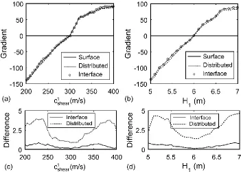
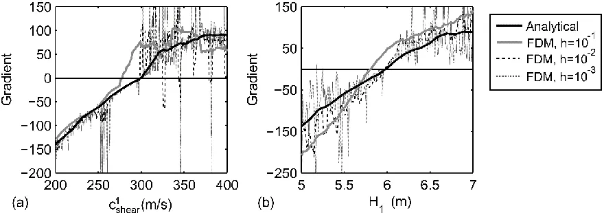
the surface, vertical load at the interface below the surface, and vertical loads distributed uniformly at all the nodes (along the depth). Figure (a) shows the gradient as a function of shear velocity of the top layer, and Figure (b) shows it as a function of thickness of the top layer (for the synthetic example, model 3 of Table 4.1). Figure (c) and (d) show the absolute difference of the gradient using the interface and distributed loads comparing to the gradient using the surface load. 81 Figure 4.7 Proposed and FDM gradients as a function of (a) shear velocity of the top layer, and
(b) thickness of the top layer (for the synthetic example, model 3 of Table 4.1). 82 Figure 4.8 Theoretical and effective dispersion curves for the synthetic example: (a) model 1,
Figure 4.9 (a) Relative norm of gradient and misfit value versus number of iterations; (b) inverted and reference effective dispersion curves; and (c) shear wave velocity profiles. ... 84 Figure 4.10 (a) Relative norm of gradient and misfit value versus number of iterations; (b)
inverted and reference effective dispersion curves; and (c) shear wave velocity profiles. ... 85 Figure 4.11 (a) Relative norm of gradient and misfit value versus number of iterations; (b)
inverted and reference effective dispersion curves; and (c) shear wave velocity profiles. ... 85 Figure 4.12 Inverted and reference shear wave velocity profiles using FDM for computing
partial derivatives for (a) model 1; (b) model 2; and (c) model 3... 86 Figure 4.13 Relative error in the phase velocity using (a) complex-length FEM with 27
elements for top three layers and 5 PMDLs for infinite layer (with relative error less than 0.1%); (b) regular FEM with 108 elements for top three layers and 20 regular FEM for infinite layer (with relative error less than 1%). ... 87 Figure 4.14 Experimental (from [127]) and inverted dispersion curves for (a) 125 μm stainless
steel plate; (b) 250 μm stainless steel plate; and (c) 210μm borosilicate glass plate. ... 88 Figure 4.15 Experimental (from [128]) and inverted dispersion curves by inverting the (a)
effective dispersion curve using the proposed derivatives and (b) effective dispersion curve using FDM derivatives. ... 90 Figure 4.16 Inverted and borehole (from [128]) shear wave velocity profiles by inverting the
(a) effective dispersion curve using the proposed derivatives and (b) effective dispersion curve using FDM derivatives. ... 91 Figure 5.1 Overview of the studied systems: (a) immersed plates; (b) immersed rods/fluid-filled pipes; and (c) immersed waveguides with arbitrary cross-section. ... 95 Figure 5.2 (a) Geometry of the immersed plate; and (b) CFEM discretization of the composite
plate. ... 96
Figure 5.3 (a) Phase velocity and (b) attenuation curves obtained by the exact solution [207] and the proposed approach (CFEM+PMDL) for the tri-laminate hard plate (Table 5.1). ... 105 Figure 5.4 (a) Phase velocity and (b) group velocity curves obtained by the exact solution [207]
and the proposed approach (CFEM+PMDL) for the tri-laminate hard plate (Table 5.3). ... 106 Figure 5.5 (a) Geometry of the immersed pipe; and (b) 1D discretization of solid and inner
fluid with high-order finite elements and linear PMDL elements for the exterior infinite fluid. ... 107 Figure 5.6 (a) Phase velocity and (b) attenuation curves obtained by the reference solution and
proposed approach (PMDL) for the tri-laminate fluid-filled and immersed hard pipe (Table 5.4). ... 110 Figure 5.7 (a) Phase velocity and (b) group velocity curves using the reference solution and
Figure 5.8 (a) Geometry of the immersed waveguide with arbitrary cross-section; (b) modeling infinite fluid with PMDL layers; and (c) integration scheme for edge and corner PMDL layers. ... 113 Figure 5.9 (a) Geometry of the bi-laminate immersed rod; (b) 2D discretization of solid cross-section (with Q8), fluid buffer region (with Q8) and infinite fluid (with PMDL 6-noded edge and 4-6-noded corner elements). Note that PMDL element lengths perpendicular to the square sides are imaginary and the illustration is schematic. ... 115 Figure 5.10 (a) Phase velocity and (b) attenuation curves obtained by the reference solution
and proposed approach (PMDL) for the bi-laminate immersed hard rod (Table 5.6). ... 115 Figure 5.11 (a) Geometry of the immersed composite rod; (b) 2D discretization of cross-section
with 4-noded complex-length elements (only real part is shown) and infinite fluid with 4-noded edge and corner PMDL elements. Note that PMDL element lengths perpendicular to the rod sides are not scaled to the rod dimensions thus the illustration is schematic... 116 Figure 5.12 (a) Phase velocity and (b) attenuation curves obtained by the reference solution
and proposed approach (PMDL) for the bi-laminate immersed soft rod (Table 5.7). ... 117 Figure 5.13 Phase velocity curves for immersed plates, (a) 210 µm thick borosilicate glass
plate and (b) 50 µm thick Plexiglass® plate, compared with the experimental results from [127] and [227], respectively. ... 118 Figure 5.14 Phase velocity curves for (a) 300 µm and (b) 150 µm immersed stainless steel
pipes compared with experimental results from [230]. ... 119 Figure 5.15 (a) phase velocity and (b) attenuation curves for 3.175×12.700 mm immersed
aluminum rod with experimental results from [231]. ... 120 Figure 6.1 Approximating the half-space by finite number of complex-length mid-point
integrated layers, truncated with a Dirichlet boundary at the end. ... 132 Figure 6.2 Approximation of the exterior stiffness by using (a) PMDL layers and (b) OSM
interface integral. ... 136 Figure 6.3 (a) Real part of a plane wave with j / 6 and (b) sine component of an interface
wave with n16. ... 138 Figure 6.4 The geometry of (a) waveguide and (b) full space problems. ... 139 Figure 6.5 Real and imaginary parts of the reference solution in the (a) waveguide and (b) full
space problems for 10 . ... 140 Figure 6.6 Number of iterations required for the convergence of PMDL and OSM methods
using the interface waves with different number of bases for: (a) waveguide and (b) full space problems. ... 143 Figure 6.7 (a) Geometry of the subsurface problem and (b) partitioning of the truncated domain
Chapter 1
Introduction
Wave propagation is the fundamental phenomenon with a broad range of applications such as geophysical exploration, structural health monitoring and biomedical imaging. The purpose of this dissertation is to devise computational strategies for forward and inverse modeling of these applications. Specifically, we develop efficient algorithms for dispersion analysis of waveguides and domain decomposition methods for parallel solution of large scale wave propagation problems.
Discussion of the presented methods and their applications are presented in Chapters 2-6 (Chapters 2-4,6 have been published and Chapter 5 will be submitted as a journal paper). Following is a summary of the contributions in each chapter.
1.1
Exponentially convergent linear finite elements
as illustration of its effectiveness for a variety of problems involving Laplace, Helmholtz and elastodynamics equations.
1.2
Dispersion analysis of embedded waveguides
Motivated by the need to compute dispersion curves for layered media in the contexts of geophysical inversion and nondestructive testing, a novel discretization approach, termed complex-length finite element method (CFEM), is developed and shown to be more efficient than the existing finite element approaches. The new approach is exponentially convergent based on two key features: unconventional stretching of the mesh into complex space and midpoint integration for evaluating the contribution matrices. For modeling the layered half-spaces of infinite depth, we couple CFEM with the method of perfectly matched discrete layers (PMDL) to minimize the errors due to mesh truncation. A number of numerical examples are used to investigate the efficiency of the proposed methods. It is shown that the suggested combination of CFEM and PMDL drastically reduces the number of elements, while requiring minor modifications to the existing finite element codes. It is concluded that the methods’ exponential convergence and sparse computation associated with linear finite elements, result in significant reduction in the overall computational cost. The reader is referred to Chapter 1 for details on the suggested methods for forward modeling of waveguides.
1.3
Near-surface imaging
method (CFEM) to model the finite depth layers, with perfectly matched discrete layers (PMDL) to model the unbounded half-space. Second, based on analytical derivatives for theoretical dispersion curves, an approximate derivative is derived for so-called effective dispersion curve for realistic geophysical surface response data. The new derivative computation has a smoothing effect on the computation of derivatives, in comparison with traditional finite difference (FD) approach, and results in faster convergence. In addition, while the computational cost of FD differentiation is proportional to the number of model parameters, the new differentiation formula has a computational cost that is almost independent of the number of model parameters. At the end, as confirmed by synthetic and real-life imaging examples, the combination of CFEM+PMDL for dispersion calculation and the new differentiation formula results in more accurate estimates of the subsurface characteristics than the traditional methods, at a small fraction of computational effort. A detailed discussion on the improved inversion algorithm is included in Chapter 4.
1.4
Dispersion analysis of immersed waveguides
parameters. Multiple numerical examples are presented to illustrate the method’s efficiency. Finally, the theoretical predications from the method are validated using experimental observations for several structural members. The reader is referred to Chapter 5 for the proposed algorithms, verification and validation.
1.5
Domain decomposition for Helmholtz problem
Chapter 2
Exponential Convergence through Linear Finite
Element Discretization of Stratified Subdomains
†
2.1
Introduction
Conventional domain-based methods such as finite element and finite difference techniques obtain the solution over the entire domain. While such approaches are appropriate for many problems, there are several situations where the response is needed only in a few small regions of interest. Some examples include: (a) reservoir modeling where the response at injection and production wells are of utmost importance, (b) forward modeling in the context of nondestructive testing and system identification, where the goal is to match the response of the system at sparse discrete points in the domain and (c) structural acoustics, where the acoustic signature is not needed at all the points, but at distinct locations in the far field. Most of these problems involve significant computational expense and it would be desirable to reduce the computational cost, if it can come at the expense of not computing the response in the rest of the domain. With this motivation, this work presents an unconventional finite element method that provides high accuracy at prescribed points in the domain. In this work, we treat the special but important class of problems involving large regular (e.g. layered) subdomains, where the actual solution inside these subdomains may not be of interest, but it is
important to capture the effect of these subdomains on the solution in the remainder of domain. Specifically, we show that a special mesh with midpoint-integrated linear finite elements results in exponential convergence of the solution on the edges of layered subdomains.
Exponential convergence is typically achieved with the help of spectral methods where the field variable is discretized with Fourier basis [1, 2], but these methods typically render the computation global. On the other hand, regular finite element and finite difference methods involve more efficient sparse computation, but the convergence is only algebraic. It was discovered that exponential convergence can be obtained with sparse computation, provided that the solution is needed only at specific points in the domain [3, 4]. By linking finite-difference approximation to rational approximation of the Dirichlet-to-Neumann (DtN) map, exponential convergence is achieved at the edges of sub-domains discretized with specially devised finite difference grids. The basic idea is to obtain optimal rational approximation of the one-sided DtN map (with Dirichlet or Neumann condition applied on the other edge), and translate the approximation to an equivalent finite difference grid. Since the grids result from exponentially convergent optimal approximations of the DtN map, they are called optimal finite difference grids and result in exponential convergence at the edges of the sub-domains. The main limitation of this method is that two distinct finite difference grids are needed, one when Dirichlet condition is applied on the other edge, and another for Neumann condition, indicating that the grids cannot be used directly for two-sided problems, which would be the building block for multi-domain problems. Optimal grids can be used for two-sided problems indirectly, through splitting the solution into odd and even parts, devising two separate grids for each part, and using them in a completely overlapping fashion. This idea is extended to multiple dimensions, but the computation becomes rather cumbersome, requiring increasing number of overlapping grids (four for two-dimensional problems and eight for three-dimensions) [4-6].
[7-9]; given the equivalence between impedance and half-space DtN map, we call this property the impedance-preserving property. We show that this property eliminates the need for multiple overlapping grids and provides exponential convergence of the DtN map for the two-sided problem with a single grid. This makes the implementation attractive and the computation can be performed by a simple modification of existing finite element codes. The only complication is that the finite element mesh needs to be bent out of the real space, making the element lengths complex-valued. This feature necessitates complex arithmetic and could contribute to an increase in the computational cost. However, this increase is not an issue as the proposed method needs a very coarse grid, with number of elements typically less by an order of magnitude than that for regular finite element discretization. Moreover, in many cases including time-harmonic wave propagation, the original computation involves complex arithmetic and the mapping of the mesh into complex space does not add any further complications.
Figure 2.1 A schematic of the model problem. An elastic layer is deforming out of plane under external excitation f0,1,2,3 at the vertical interfaces. The segments bounded by these interfaces can be stratified in the vertical direction. The goal is to obtain the responses at the
interfaces.
Section 2.3.1, as Crank-Nicolson discretization of an equivalent first-order system (Section 2.3.2). Exponential convergence is achieved by choosing the parameters by linking the Crank-Nicolson discretization with Padé approximants (Section 2.3.3). The result is a finite element mesh with complex element lengths, as discussed in Section 2.3.3. In Section 2.4 we show the applicability of the present method to general vector (elastic) equations. Section 2.5 contains numerical examples illustrating the exponential convergence and practical use of the proposed method.
2.2
Preliminaries
2.2.1 Problem statement
For the sake of focused discussion, consider the model problem in Figure 2.1, where an elastic layer with three segments, each individually stratified in the vertical direction. Excitation is applied only at the vertical edges and interfaces, and the goal is to obtain the response at these locations. We consider the anti-plane shear deformation governed by the Helmholtz equation (Laplace equation being a special case when frequency 0):
2, w , w , 0
G x z G x z x z w
z z x x
, (2.1)
0,0, 2
0
Obtain the relationship DtN: , with satisfying:
0 ,
0, for
0 , 0, 0. x L x L z z H dw w w dx x L w w
G z G z z w
z H
z z x x
w w z
Problem 1 : (2.2)
2.2.2 Dimensional reduction
Our ultimate goal is to obtain a finite element mesh that can yield accurate results at the vertical interfaces. Assuming that accuracy is needed along the entire length of every interface, we perform z discretization in a conventional manner and independent of x coordinate. It is also natural to make x discretization independent of z, resulting in a two-dimensional tensor-product mesh. For the purposes of analyzing the method, the tensor tensor-product discretization can be viewed as discretization in z followed by discretization in x. In this subsection, we focus on the discretization in z and the resulting dimensionally reduced differential equation in x. Dimensional reduction is performed by (a) multiplying the governing equation (2.2) by virtual displacement by w, (b) performing integration by parts in z , and (c) applying the boundary conditions at z0, H , resulting in:
2 2
2 0
0 for all , 0
z L
z
w w w
G z wG z w z w dz w x L
z z x
. (2.3)We apply Bubnov-Galerkin method, i.e. use the following approximations, ( ) ( ) and ( ) ( )
z z
wN z W x wN z W x , (2.4)
where Nz is the matrix of interpolation functions (shape function matrix), and W and W
2
2
2 , for 0 ,
d
x L dx
W
RW H MW 0 (2.5)
where,
0 0 0
, , .
T
z H z H z H
T T
z z
z z z z
z z z
G dz G dz dz
z z
N N
R H N N M N N (2.6)
Equation (2.5) can be decoupled into a set of differential equations through eigen-decomposition:
2
min max
2 0 for 0 ,
l
l l l
u
u x L
x
, (2.7)
where l are the eigenvalues of H with respect to R2M. ul are the weights of the corresponding eigenvectors (modal participation factors). Note that l are real and bounded
because all the matrices are symmetric and A is positive definite.
With the above decoupling, the original problem of obtaining the two-dimensional DtN map simplifies to finding the DtN maps for a set of one-dimensional boundary value problems:
0,
0, 2
min max 2
Obtain the relationship DtN: , with satisfying:
0 for 0 , .
x L x L du u u dx u
u x L
x
Problem 2 : (2.8)
Note that the subscript l is not shown this point forward for simplicity in presentation. For the special case of homogeneous media, the shape functions Nz can be chosen according to Fourier expansion, directly resulting in decoupled system of equations in (2.7). Nevertheless, we use general discretization in the z direction, to ensure applicability to stratified media. Note that eigen-decomposition leading to (2.7) is performed only for the purposes of analyzing the method; it is never performed in the actual computation.
2.2.3 A closer look at the DtN map
00 0 0 0 0 L L LL L L K K v u K K v u K
, (2.9)
where v u x and the subscripts represent the locations at which the quantities are evaluated. The negative sign for v0 is because the outside normal at x0 is in the negative x direction. Considering the geometric symmetry of the domain as well as the symmetry of the operator, the DtN map takes the form,
diag off off diag K K K K
K . (2.10)
For a fixed, the exact DtN map can be easily obtained by solving the two-point boundary value problem in (2.8), and is given by,
diag off exact
off diag
cosh 1
sinh 1 cosh
L
K K
K K L L
K . (2.11)
Note that the exact DtN map satisfies the impedance-preserving property, defined as follows: when Kexact is augmented with the exact DtN map of a half-space
Khalfspace
and the interior node is eliminated, exact half-space stiffness (and thus impedance) is preserved at the exterior node (this follows from the simple physical argument that when a layer is added to a half-space with same material properties, we obtain the same half-space). In other words, impedance preserving property states that, when a layer
x x0, 1
is augmented with a half-space
x1,
, the Neumann data required at x0 to generate a Dirichlet data of u0 is Khalfspaceu0 , i.e.,diag off 0 halfspace 0 off diag halfspace 1 0
K K u K u
K K K u
. (2.12)
It is easy to show that the above definition is equivalent to,
2 off halfspace diag diag halfspace K K K K K Noting that Khalfspace , it is easy to see that impedance-preserving property takes the simple form,
2 2
diag off
K K . (2.14)
discretization of the real domain
0,L
, but a mesh mapped into the complex space (the element lengths are complex-valued). We thus term this the Complex-length Finite Element Method (CFEM); the remainder of the chapter contains the formulation of CFEM and the illustration of its effectiveness.2.3
Complex-length finite element method (CFEM)
2.3.1 Linear finite elements with midpoint integration
Consider the domain
0,L
discretized into non-overlapping finite elements of lengths , 1, ,j
L j n,
Lj L, with nodes located at x0, x1,..., xn. Restricting the discussion to the jth element, the weak form becomes,1
1 1
j
j x
j j j j
x
u u
u u dx u v u v x x
, (2.15)where u is the variation of u. Utilizing Bubnov-Galerkin method with linear interpolation within the element and after performing the transformation x x xj1, we obtain,
1 1 1 1
0
1 1 1 1
1 1
j
T L T T T
j j j j j j j j
j j j j j j j j
u L L x L x L u u v
dx
u L L x L x L u u v
. (2.16)The next step is to evaluate the integral using the midpoint rule. Performing such integration and eliminating the virtual displacements, we obtain the DtN map (stiffness relation) for a single element: 1 1 1 1 4 4 1 1 4 4 j j j j j j
j j j j
j j
L L
L L
v u
v L L u
L L
. (2.17)
In the above DtN map, 2 2 diag off
(see (2.14)). Since all the finite elements in the mesh satisfy this property, the two-point DtN map of the entire mesh would also satisfy the impedance-preserving property. An important consequence is that, a mesh that results in exponential convergence of the diagonal element of the DtN map, also results in exponential convergence of the off-diagonal element (this is
because, 2 2 2 2
diag, approx off, approx diag, exact off, exact
K K K K ), and thus exponential convergence of the entire two-sided DtN map.
To obtain the DtN map of the discretized domain, we could assemble the 2 2 DtN maps of the individual elements and eliminate the interior degrees of freedom by taking Schur complement. This process renders the computation global, making it cumbersome to analyze. To facilitate easier analysis, we turn to an equivalent propagator matrix approach, by converting the boundary value problem into an initial value problem.
2.3.2 An alternative view: first-order form
We can verify that the DtN relation in (2.17) is equivalent to, 1 1 1 1 0 2 0 2 j j j j j
j j j j
j
u u u u
L
v v v v
L
, (2.18)
where v v . It can be immediately seen that the above equation is the Crank-Nicolson discretization of first order form of differential equation (2.7), i.e.,
min max 0
for 0 ,
0 u u x L v v x
. (2.19)
Equation (2.18) can also be written in the form, 1 1 j j j j j u u v v
P , (2.20)
the propagator matrix of the complete interval
0,L
, P, is obtained by simply multiplying the propagator matrices of individual finite elements:1 2 0
1 1 2 1
1 2 0
n n
L
n n n n n
n n
L
u u u
u
v v v
v
P P P P P P P
P
. (2.21)
The matrix P can also be written in the form of DtN relation in (2.9), implying that successful approximation of the propagator matrix would automatically result in successful approximation of the DtN map. Thus, the problem reduces to, finding the mesh parametersLj that would result in exponential convergence of the propagator matrix P for various values of
on the real line.
The problem of approximating the propagator matrix can be further simplified by decoupling the system of equations in (2.19). Through eigen-decomposition, we have,
1 1
min max
2 2
0
for 0 ,
0 x L x
, (2.22)
where the diagonal matrix contains the eigenvalues of the operator in (2.19), and 1, 2 are the weights associated with the corresponding eigenvectors. Thus the DtN approximation problem reduces to:
max max
min min
Find the mesh parameters that would result in exponentially convergent propagator matrix for the interval (0, ) for the equation:
for all , , .
j L L i i x
Problem 3 :
(2.23) In the above, and min is implicitly assumed to be negative, indicating that could be imaginary. It is instructive to note the physical meaning of the eigenvectors associated with the decoupled form in (2.22). The eigenvector associated with 1 is
u v
1 1 , or equivalently, v u, which corresponds to an exponentially growing solution, 1 xue . The other eigenvector is
u v
1 1
, which corresponds to a decaying solution, 2 x. These are the solutions of the original second order differential equation (2.7). This point of view is important as our method is based on approximation of the exponential functions (see Section 2.3.3).
The impedance-preserving property of the midpoint-integrated linear finite elements can be proven more elegantly as follows. The impedance relation for the half-space (0, ) is:
0 0
x
u x u
, or v0 u0 (this corresponds to the decaying solution). The impedance-preserving property can be stated as: exact impedance relation v u at x0 implies v u at any x. The impedance-preserving property of the exact propagator can be illustrated as follows: Equation (2.19) is invariant to the swapping of u with v ; therefore, if the initial condition at x0 is swap-invariant (v u), the “final” condition at any x must also be swap-invariant (v u). Fortunately, the swap-invariance of (2.19) is preserved through the discretization in (2.18), implying that the Crank-Nicolson propagator, and thus the midpoint-integrated finite element, satisfy the impedance-preserving property.
2.3.3 Selection of the mesh parameters
Considering that the exact solution to (2.23) is of the form Aex, the propagator associated with the interval
0,L
is simply,0
L L exact
P e
. (2.24)
The approximate propagator for the jth interval is given by the Crank-Nicolson method,
1 1
1
1 2
2 1 2
j
j j j j j
j j j j L L L P
. (2.25)
The propagator for the entire interval
0,L
is the product of all the propagators, i.e.,1 1 1 2 1 2 n n j approx j
j j j
L P P L
. (2.26)the form Q( ) Q(), where Q is a polynomial of degree n with roots 2 Lj. Relative approximants are well-studied subject of rational approximation theory [13], and there is a variety of approximants convergent on the real axis at least exponentially with respect to n. Obviously, Q( ) Q() must not have poles and residues on the real axis in order to be a good approximant of the exponent there; this is the reason why Lj must be complex, implying that the mesh has to be mapped into the complex space. Hence the current method is called the Complex-length Finite Element Method (CFEM).
In this work, we consider the relative (diagonal) Padé approximant matching the first 2n terms of Taylor expansion at 0. In other words, the 0 to 2nth derivatives of the approximant must match with that of the exact solution at 0, i.e.,
0 0
, 0, , 2
j L
j pade
j j
d e d P
j n
d d
. (2.27)
The reason for the choice of Padé approximant is its simplicity. There are a number of approximants of the form ( )Q Q() with better convergence properties for larger ; we plan to consider such approximations in future research.
For the Padé approximant considered in (2.27), the roots 2 Lj and thus the element lengths Ljcan be computed with a standard algorithms (see e.g. [14]). The resulting mesh has the following properties:
1. Lj are independent of (or ), indicating that the same mesh can be used for the range of complex given in (2.8), implying that the mesh is applicable to the original 2D problem in (2.2).
2. Lj come in complex conjugate pairs. It follows from the fact that the Padé approximant is real for any real .
analysis domain.
4. A peculiar property of midpoint-integrated finite element grid is that the DtN map is invariant of the ordering of the elements. This implies that the mesh is not unique; we order the mesh so that it is symmetric and smooth (as smooth as possible) in the complex plane. Such a mesh is obtained by ordering the elements with increasing or decreasing phase angle of their lengths (see Section 2.5.2).
5. The mesh scales with the length of the domain and we can tabulate the element sizes relative to the domain size, i.e. Lj L, for any given number of elements; this is done in Table 2.1 Element lengths for varying number of elements ( )n . The domain size is unity. For other cases, the element lengths simply scale with domain size. up to 16 elements. In general one can obtain Lj L2 /xj where xj are the roots of the
th
n -degree polynomial (see e.g. [14]):
0
(2 )!
( ) 0.
! ( )!
n
j j
n j x j n j
(2.28)Following the order suggested in item 4 above, the meshes are shown Figure 2.2. Meshes with odd and even number of elements are shown in separate figures for clarity in presentation. With refinement, the mesh appears to converge to a specific curve in the complex space. We suspect that there is an analytical form for the converged mesh, linked to the asymptotic behavior of the poles of Padé approximants, similar to the one known for optimal approximants on [0, ) [15].
Table 2.1 Element lengths for varying number of elements ( )n . The domain size is unity. For other cases, the element lengths simply scale with domain size.
1
n 1.00000000000000 n2 0.50000000000000 0.28867513459481 i
3
n 0.28468557688388 0.27159985141630 0.43062884623222
i
4
n 0.18313248053143 0.23132522602625 0.31686751946856 0.09488202514221 i i 5 n
0.12803667831541 0.19668213834621
0.23485450871940 0.12209940763707 0.27421762593037
i i
n6
0.09489061789607 0.16944514819433
0.17914640739749 0.12594324946340 0.22596297470643 0.04614135671779 i i i 7 n
0.07338559568636 0.14811940741461
0.14065739395847 0.12154781833235
0.18538954553266 0.06776497788782
0.20113492964499 i i i
n8
0.05861791492234 0.13119236974564
0.11325833004971 0.11445496413908
0.15337794771885 0.07709430353886
0.17474580730908 0.02713226173787 i i i i 9 n
0.04802049907890 0.11752570488080
0.09316287173966 0.10679717990370
0.12840441052931 0.08014721079992 0.15100957026047 0.04281546509628
0.158805296783284 i i i i 10 n
0.04014472910062 0.10630697796687
0.07802273616547 0.09940003581225
0.10881874816902 0.07996015060428 0.13078256453612 0.05163001172938
0.14223122202876 0.01782841382104 i i i i i 11 n
0.03412261657800 0.09695789626293 0.06634486381072 0.09256005182226
0.09329088025857 0.07811366645707
0.11386072467713 0.05628616844255 0.12678425930221 0.02942684799389
0.1311933107466 i i i i i 99 12 n
0.02940803944815 0.08906181395662 0.05715192456673 0.08635352530097
0.08082582076929 0.07545289071966
0.09976290741316 0.05839885662872 0.11301395814524 0.03687019624343
0.1198373496574 i i i i i
1 0.01259866487095 i
13 n
0.02564318775369 0.08231355321087 0.04978573946440 0.08076582096948
0.07069390925651 0.07243833050796
0.08799247146698 0.05894563008011 0.10097469339377 0.04152986688324
0.1090297769962 i i i i i
7 0.02144314210934
0.11176044333671
i
14 n
0.02258550311646 0.07648569373967 0.04379127631258 0.07574740948845
0.06236027779351 0.06932300610809
0.07811546938314 0.05852853926583 0.09053178744825 0.04431195125450
0.0991146446092 i i i i i
7 0.02760255210502
0.10350104133675 0.00937153174338 i i
15 n
0.02006570730347 0.07140591920396 0.03884638966705 0.07123849065223
0.05542991160544 0.06624511011050
0.06977487505357 0.05752432367232 0.08149231310591 0.04581962272804
0.0901849036901 i i i i i
5 0.03183750267162
0.09553514496841 0.01630985840134 0.09734150921194 i i 16 n
0.01796266496341 0.06694162366630 0.03471809507502 0.06717964470869
0.04960794930403 0.06327803486714
0.06268398209122 0.05617188543383 0.07365957371625 0.04645858465651
0.0822166735093 i i i i i
8 0.03468717833984
0.08808374597041 0.02141958057287 0.09106731537025 0.00724175169196 i i i
Figure 2.2 Finite element meshes for (a) odd number of elements and (b) even number of elements.
2.3.4 Summary: CFEM discretization procedure and additional properties
We suggest the following approach for CFEM discretization of the model problem in Figure 2.1:
3. Combine all the sub-domain grids and perform finite element analysis on the entire domain. Utilize midpoint integration to evaluate the contribution matrices.
4. Extract the results from the sub-domain interfaces. Note that the displacements in the interior of the sub-domains have no immediate physical meaning.
It is also worth mentioning that CFEM also satisfies the following important properties: 1. CFEM is a standard finite element method, but with complex coordinate stretching.
Thus, it shares similarities with perfectly matched layers (PML) used in unbounded domain modeling, which can also be viewed in terms of complex coordinate stretching [17]. The difference is that PML stretching leaves invariant one boundary point, whereas both boundary points are invariant in our method. PML finite elements lengths do not come in conjugate pairs and the one-sided DtN map is not Hermitian, consistent with PML’s need to absorb energy. On the other hand, our method propagates all the information from one end of the domain to the other end without any loss of energy. This is because, although our stiffness matrix is complex symmetric, the two-sided DtN map for the entire mesh is real symmetric (Hermitian) due to complex conjugate pairs of element lengths, as shown in Appendix A.
considered in [11]. Reference [11] also shows the equivalence of Padé finite-difference scheme and the spectral Galerkin method with polynomial basis functions, again in terms of the DtN maps.
3. The stiffness matrix from discretization of elliptic equations, i.e. Equation (2.8) with 2
0
, while not Hermitian, is semi-positive stable, i.e., the real part of the eigenvalues of the stiffness matrix is equal or greater than zero. Appendix C contains the proof of this property.
While the discussion is limited to Laplace and Helmholtz equations, the mesh should also work for hyperbolic problems such as the wave equation. Since for CFEM, the generalized eigenvalues of the stiffness matrix with respect to the mass matrix are non-negative and real, traditional time-stepping methods would be stable. The only drawback of CFEM for hyperbolic problems is that the mass matrix is not diagonal (due to midpoint integration). However, it could be block diagonal, as the degrees of freedom are coupled only in the x direction; mass lumping can be performed in the z direction. Fortunately, exponential convergence of the proposed method facilitates drastic reduction in the number of elements in the x direction, which translates into small block size and efficient computation.
There may be concern associated with the increased cost due to complex arithmetic. We note that this cost increase is negligible compared to the savings from significant reduction in the number of degrees of freedom facilitated by exponential convergence. Moreover, many problems involving wave propagation require complex arithmetic and complex element lengths do not increase the computational cost for these problems.
The method in the presented form is applicable to problems where the solution is needed on the edges of the subdomains. If the solutions are needed only at the corner points, if the domain geometry allows, the CFEM discretization can also be used in the transverse direction (if the material properties are pricewise constant in that direction), resulting in further reduction in the computational cost.
electromagnetism and elasticity (similar to the development for finite difference schemes in [5, 6, 12]). We illustrate the applicability of the proposed approach for the special case of elastodynamics in the next section. In addition, successful application of CFEM for solving the eigenvalue problems associated with elastic layered (stratified) media can be found in [19, 20].
2.4
CFEM for vector equations (elastodynamics)
We generalize CFEM for solving linear elastodynamics problems. In particular, we prove the impedance-preserving property for elastodynamics equation, and derive associated propagation factors. By observing that these propagation factors are identical to those in scalar analysis, we conclude that CFEM is applicable to vector wave equations.
2.4.1 Model Problem
Consider a two-dimensional elastic layered medium with in-plane deformation as shown in Figure 2.1. Each layer is assumed to be homogeneous, but the material properties may vary between different layers. The equation representing in-plane wave propagation for the harmonic waves of the form u x( , )t u x( , ) ei t u k( , ) eik x i t with no external body forces and damping, can be written as,
2
, T
s
σ u 0 (2.29)
where T [ / 0 / ; 0 / / ]
s x z z x

![Figure 3.4 (a) Mid-point integrated layer [0, ]L plus the half-space [ ,L and (b) the entire )](https://thumb-us.123doks.com/thumbv2/123dok_us/1619068.1201127/65.612.95.541.450.656/figure-mid-point-integrated-layer-plus-space-entire.webp)