ABSTRACT
BOBINYEC, KAREN S. Observer Construction for Systems of Differential Algebraic Equations using Completions. (Under the direction of Dr. Stephen L. Campbell.)
This dissertation presents the results from researching observer construction for systems of differential algebraic equations using completions. Physical systems of interest in control theory are sometimes described by ordinary differential equations (ODEs) and algebraic equations, forming a system of differential algebraic equations (DAEs). Challenges from solving a system of DAEs come from the first derivative of its state vector having a singular coefficient matrix and from possibly implicit algebraic constraints defining its solution manifold. These challenges exist for observing a system of DAEs as well, leading to processes that require the system to meet certain assumptions.
© Copyright 2013 by Karen S. Bobinyec
Observer Construction for Systems of Differential Algebraic Equations using Completions
by
Karen S. Bobinyec
A dissertation submitted to the Graduate Faculty of North Carolina State University
in partial fulfillment of the requirements for the Degree of
Doctor of Philosophy
Applied Mathematics
Raleigh, North Carolina 2013
APPROVED BY:
Dr. Robert H. Martin Dr. Ralph C. Smith
Dr. Hien T. Tran Dr. Stephen L. Campbell
DEDICATION
BIOGRAPHY
ACKNOWLEDGEMENTS
I would like to acknowledge
Dr. Stephen Campbell, who was willing to be my advisor;
Dr. Robert Martin, for without his classes, I might not have remained in graduate school;
Dr. Kimberly Drake for the internship at NAVSEA in Philadelphia, PA;
my committee members and grad. school representative for being flexible with scheduling;
my Meredith College professors in mathematics, history and politics, and the Honors Program for inspiring me to continue learning and for their dedication to their students;
my parents John and Susan Bobinyec, my grandmother Berniece Stoops, and my friends Jennifer Rowland, Amanda Beasley, Sejal Patel, Martene Fair Stanberry, and Ellen Pe-terson Swanson for their support;
friends, officemates Kim Spayd and Chuck Wessell for picking me to be their third wheel;
TABLE OF CONTENTS
LIST OF TABLES . . . vii
LIST OF FIGURES . . . .viii
Chapter 1 Introduction . . . 1
Chapter 2 Completions . . . 6
2.1 Least Squares Completion . . . 7
2.2 Stabilized Least Squares Completion . . . 8
2.3 Alternative Stabilized Completion . . . 9
2.3.1 Linear Time-Invariant Case . . . 10
2.3.2 Linear Time-Varying Case . . . 14
2.4 Completion Stability . . . 15
Chapter 3 Observers . . . 17
3.1 Observable and Detectable . . . 17
3.2 The Full-Order Observer . . . 19
3.2.1 Linear Time-Invariant Case . . . 20
3.2.2 Linear Time-Varying Case . . . 22
3.3 The Reduced-Order Observer . . . 25
3.3.1 Linear Time-Invariant Case . . . 25
3.3.2 Linear Time-Varying Case . . . 28
3.4 The Maximally Reduced Observer . . . 34
3.5 DAE Manifold Observer . . . 36
3.6 Completion Stability Revisited . . . 38
Chapter 4 Theory. . . 39
4.1 Completions and Observability . . . 39
4.2 Full-order and Reduced-order Observers . . . 44
4.3 Comments on Linear Time-Varying Theory . . . 49
Chapter 5 Linear Time-Invariant Example . . . 52
5.1 Mechanics Example Introduction . . . 52
5.2 Observer Implementation . . . 54
5.3 Observer Construction Code . . . 83
Chapter 6 Linear Time-Varying Example . . . 85
6.1 Circuit Example Introduction . . . 85
6.2 Observer Implementation . . . 91
6.2.1 Example with Positive Resistors . . . 92
6.2.2 Example with Negative Resistors . . . 143
Chapter 7 Conclusions, Contributions, and Future Research Topics . . . .184
7.1 Conclusions . . . 184
7.2 Contributions . . . 186
7.3 Future Research Topics . . . 187
REFERENCES . . . .189
APPENDICES . . . .201
Appendix A Smooth Decomposition . . . 202
A.1 Smooth Decomposition . . . 202
A.2 First Derivatives . . . 206
A.3 Alternatives to the Smooth Decomposition . . . 211
Appendix B MATLAB Code . . . 212
B.1 Chapter 5 Code . . . 212
B.2 Chapter 6 Code . . . 252
LIST OF TABLES
Table 6.1 For each ΛSL, the number of Ae(t)’s eigenvalues with a negative real part. . 98
Table 6.2 For each ΛSL, the ranks of Wo(t) and their time intervals for two output
matrices. . . 98 Table 6.3 For each ΛSL, the ranks ofWo(t) and their time intervals for output matrix
Cc. . . 99 Table 6.4 For each ΛA, the number ofAe(t)’s eigenvalues with a negative real part. . 102
Table 6.5 For each ΛA, the ranks of Wo(t) and their time intervals for two output
matrices. . . 103 Table 6.6 For each ΛA, the ranks ofWo(t) and their time intervals for output matrix
Cc. . . 103 Table 6.7 For each ΛSL, the number of Ae(t)’s eigenvalues with a negative real part. . 147
Table 6.8 For each ΛSL, the ranks of Wo(t) and their time intervals for two output matrices. . . 148 Table 6.9 For each ΛSL, the ranks ofWo(t) and their time intervals for output matrix
Cf. . . 148 Table 6.10 For each ΛA, the number ofAe(t)’s eigenvalues with a negative real part. . 151
Table 6.11 For each ΛA, the ranks of Wo(t) and their time intervals for two output
matrices. . . 152 Table 6.12 For each ΛA, the ranks ofWo(t) and their time intervals for output matrix
LIST OF FIGURES
Figure 5.1 x(t), solution of system (5.4). . . 57 Figure 5.2 xe(t), completion solutions of system (5.4). . . 58 Figure 5.3 x(t)−xe(t), comparing exact solution with completion solutions. . . 58 Figure 5.4 SLSC/FO, ASC/FO observers plotted with solution x(t). (Ca, λ = 2,
ρ=−1) . . . 63 Figure 5.5 x(t)−xb(t) comparison. (Ca,λ= 2, ρ=−1) . . . 64 Figure 5.6 LSC/MR observer’s x(t)−xb(t); the MR observer differences are SLSC –
ASC and SLSC – LSC. Neither the completion nor λ influences the MR observer. (Ca,λ= 0,λ= 2,ρ=−1) . . . 64 Figure 5.7 x(t)−xb(t) progression as ρ is varied, 2nd component ofx1(t). (Ca,λ= 2) 66 Figure 5.8 x(t)−xb(t) progression as ρ is varied, 1st component ofx2(t). (Ca λ= 2) . 66 Figure 5.9 x(t)−xb(t) progression as ρ is varied,x3(t). (Ca,λ= 2) . . . 67 Figure 5.10 x(t)−xb(t) progression asλis varied, 2nd component ofx1(t). (Ca,ρ=−1) 67 Figure 5.11 x(t)−bx(t) progression as λis varied, 1st component of x2(t). (Ca,ρ=−1) 68 Figure 5.12 x(t)−xb(t) progression as λis varied,x3(t). (Ca,ρ=−1) . . . 69 Figure 5.13 q(t) (solid) and qb(t) (dashed) for two extended output matrices. (Ca,
ρ=−1) . . . 70 Figure 5.14 MR observers’q(t)−qb(t) for two extended output matrices. (Ca,ρ=−1) 70 Figure 5.15 x(t) (solid) andxb(t) (dashed) for two extended output matrices; the MR
observer difference is (CΞ, Ca)−(CΞ,GF). The results in terms of x(t),
b
x(t) are the same. (Ca,ρ=−1) . . . 70 Figure 5.16 x(t)−xb(t) comparison. (Cc,λ= 2, ρ=−1) . . . 73 Figure 5.17 x(t)−xb(t) progression as ρ is varied, 1st component ofx1(t). (Cc,λ= 2) 75 Figure 5.18 x(t)−xb(t) progression as ρ is varied, 2nd component ofx2(t). (Cc,λ= 2) 75 Figure 5.19 x(t)−xb(t) progression as ρ is varied,x3(t). (Cc,λ= 2) . . . 76 Figure 5.20 x(t)−xb(t) progression asλis varied, 1st component ofx1(t). (Cc,ρ=−1) 76 Figure 5.21 x(t)−xb(t) progression asλis varied, 2nd component ofx2(t). (Cc,ρ=−1) 78 Figure 5.22 x(t)−xb(t) progression as λis varied,x3(t). (Cc,ρ=−1) . . . 78 Figure 5.23 Solution p(t) and DAE/M observer pb(t) plotted together; DAE/M
ob-server’s p(t)−pb(t). (Ca,ρ=−1) . . . 80 Figure 5.24 Solutionx(t) and DAE/M observer’s bx(t) plotted together; DAE/M
ob-server’s x(t)−bx(t). This observer’s e(t) is comparable to the e(t) for the ASC/FO observer with Cc,λ= 2, ρ=−1. (Ca,ρ=−1) . . . 81 Figure 5.25 x(t)−xb(t) progression as ρ is varied, DAE/M observer. (Ca) . . . 81 Figure 5.26 Solutionx(t) and DAE/M observer’s bx(t) plotted together; the DAE/M
observer difference is Ca −Cc. The DAE/M observers are the same for Cases 1 and 3. . . 81 Figure 5.27 Solutionx(t) and DAE/M observer’s bx(t) plotted together; DAE/M
Figure 6.3
Ae(t)
for five choices of ΛSL. Each Ae(t)
is bounded. . . 96
Figure 6.4
Be(t)
for five choices of ΛSL. Each Be(t)
is bounded. . . 97
Figure 6.5 kΦ(t,0)kon two intervals of time. kΦ(t,0)k −→0 for each choice of ΛA. . 100 Figure 6.6
Ae(t)
for five choices of ΛA. Each Ae(t)
is bounded. . . 101
Figure 6.7
Be(t)v(t)
for an SLSC and an ASC. Be(t)
cannot be computed for the
ASC, but comparing
Be(t)v(t)
for the stabilized completions suggests
the ASC
Be(t)
is bounded. . . 101
Figure 6.8 kΦ(t,0)kfails to converge to zero for the LSC (ΛL). . . 104 Figure 6.9
Ae(t)
and
Be(t)
are bounded for the LSC (ΛL). . . 104
Figure 6.10 SLSC solution (Λ4SL) on two intervals of time. Figure 6.10b suggests system (6.9)’s solution is periodic. . . 106 Figure 6.11 The ASC solution (Λ4A) is comparable to the SLSC solution in Figure
6.10. The solution difference is SLSC – ASC. . . 106 Figure 6.12 The LSC solution (ΛL) is comparable to the SLSC solution in Figure 6.10.
The solution difference is SLSC – LSC. . . 106 Figure 6.13 SLSC/FO observer’s xe(t)−xb(t) on two intervals of time. e(t) −→ 0 by
t= 135. (Ca, Λ4SL,δ = 0.1,η= 1, ξ= 0.1) . . . 108 Figure 6.14 SLSC/FO observer’s ex(t)−xb(t) on two intervals of time; SLSC solution
and FO observer plotted together. e(t) −→ 0 by tf = 45. (Ca, Λ4SL,
δ = 0.1,η= 100, ξ = 0.1) . . . 109 Figure 6.15 ASC/FO observer’sxe(t)−xb(t) on two intervals of time; ASC solution and
FO observer plotted together. e(t) −→ 0 bytf = 45. (Ca, Λ4A, δ = 0.1,
η = 100, ξ= 0.1) . . . 109 Figure 6.16 Observer comparison. SLSC/FO and ASC/FO observers plotted together;
the observer difference is SLSC/FO – ASC/FO. (Ca, Λ4SL, Λ4A,δ= 0.1,
η = 100, ξ= 0.1) . . . 109 Figure 6.17 xe(t)−xb(t) progression asη is varied, SLSC/FO observer. Shortened time
intervals provide closer views of initial differences. (Ca, Λ4SL, δ = 0.1,
ξ = 0.1) . . . 110 Figure 6.18 SLSC/FO observers’ ex(t)−xb(t) asδ and η are varied. These estimation
errors appear to be the same. (Ca, Λ4SL,ξ= 0.1) . . . 111 Figure 6.19 δ = 0.01 SLSC/FO and η = 10 SLSC/FO observers plotted together;
the SLSC/FO observer difference is (δ= 0.01)−(η= 10). Shortened time interval shows observers are not the same usingiv(t) estimates as example.
(Ca, Λ4SL,ξ = 0.1) . . . 111 Figure 6.20 SLSC/FO observer’s ex(t) − xb(t); the SLSC/FO observer difference is
(ξ= 0.01)−(ξ = 0.1). Decreasingξ does not visibly affect SLSC/FO ob-server convergence. (Ca, Λ4SL) . . . 113 Figure 6.21 SLSC/FO observer’sex(t)−xb(t) for Λ2SL; Λ2SL, Λ4SL SLSC/FO observers
plotted together. Effects from changing ΛSL are visible on t∈[0,2]. (Ca,
Figure 6.22 SLSC/FO observers’xe(t)−xb(t) as δ and ξ are varied. (Ca, Λ4SL,η= 100) 113 Figure 6.23 Solution comparison. The ASC solution difference is SDM – SYM. (Λ4A) . 114 Figure 6.24 Observer comparison. ASC/FO SDM observer’sxe(t)−xb(t); the ASC/FO
observer difference is SDM – SYM. (Ca, Λ4SL,δ= 0.1,η= 100, ξ = 0.1) . 115 Figure 6.25 LSC/FO observer’sex(t)−bx(t) on two intervals of time. e(t) fails to
con-verge to zero by t= 90. (Ca, ΛL,δ= 0.0001, η= 100, ξ = 0.1) . . . 116 Figure 6.26 LSC/FO observers’xe(t)−xb(t) asηis varied. Increasingη does not result
in e(t)−→0 by tf = 45. (Ca, ΛL,δ = 0.1,ξ= 0.0001) . . . 117 Figure 6.27 LSC/FO observer’s xe(t)−bx(t) on three intervals of time. e(t) fails to
converge to zero by t= 90. (Ca, ΛL,δ= 0.1, η= 1000,ξ= 0.0001) . . . . 117 Figure 6.28 SLSC/RO observer’sxe(t)−bx(t) on two intervals of time; SLSC/RO
ob-server’s q(t)−qb(t). Transformation matrix R is a permutation matrix. (Ca, Λ4SL,δ = 0.1,η= 1,ξ = 0.1) . . . 119 Figure 6.29 ASC/RO observer’s ex(t) −xb(t) on two intervals of time; ASC/RO
ob-server’sq(t)−qb(t). The order of the observer is reduced from 6 to 2. (Ca, Λ4A,δ = 0.1,η= 1, ξ= 0.1) . . . 119 Figure 6.30 ASC/RO observer’sex(t)−xb(t) on two intervals of time. Integration
tol-erance error occurs for SLSC/RO observer (Λ4SL) and same δ,η, and ξ. (Ca, Λ4A,δ= 1,η = 1,ξ = 1) . . . 121 Figure 6.31 kΦR(t,0)kis bounded; LSC/RO observer’sxe(t)−bx(t) on two intervals of
time. e(t) −→ 0 by tf = 45 for an LSC/RO observer. (Ca, ΛL,δ = 0.1,
η = 1000,ξ= 0.0001) . . . 121 Figure 6.32 xe(t)−x(t); equation (6.13) computesx(t) without observer. (Ca) . . . 121 Figure 6.33 SLSC/FO observers’ ex(t)−xb(t) forCb and Cc. (Λ4SL,δ = 0.1,η = 100,
ξ = 0.1) . . . 122 Figure 6.34 SLSC/FO observers’ xe(t)−xb(t) as η is varied. For output matrix Cc,
increasingηmay not improve observer convergence. (Λ4SL,δ= 0.1,ξ= 0.1)123 Figure 6.35 xe(t)−xb(t) progression as η is varied, SLSC/FO observer with output
matrix Cc. Effects on state variable estimates are not uniform when in-creasing η. (Λ4SL,δ= 0.1,ξ = 0.1) . . . 123 Figure 6.36 SLSC/FO observers’ ex(t) −xb(t) as η is varied. For output matrix Cb,
increasing η leads toe(t)−→0 monotonically. (Λ4SL,δ = 0.1,ξ= 0.1) . . 124 Figure 6.37 The SLSC/FO observer difference isCb−Ccasηis varied. The SLSC/FO
observer with output matrix Cb converges to xe(t) faster. (Λ4SL,δ = 0.1,
ξ = 0.1) . . . 124 Figure 6.38 SLSC/RO observers’ q(t)−bq(t) for Cb and Cc. (Λ4SL, δ = 0.1, η = 1,
ξ = 0.1) . . . 126 Figure 6.39 SLSC/RO observers’q(t)−qb(t) forCbandCc. Shortened time intervals for
results from Figure 6.38 show each reduced-order observer is estimating just the unmeasurable components of its transformed state vector. (Λ4SL,
δ = 0.1,η= 1, ξ= 0.1) . . . 126 Figure 6.40 SLSC/RO observers’ ex(t)−xb(t) for Cb and Cc. (Λ4SL, δ = 0.1, η = 1,
Figure 6.41 SLSC/RO observers’xe(t)−xb(t) asη is varied. For output matrixCc, in-creasingηexchanges an estimate’s accuracy for faster convergence. (Λ4SL,
δ = 0.1,ξ = 0.1) . . . 127 Figure 6.42 SLSC/RO observers’xe(t)−xb(t) as η is varied. For output matrix Cb, a
maximumη may exist for convergence to occur by a specific time. (Λ4SL,
δ = 0.1,η= 0.1) . . . 127 Figure 6.43 xe(t)−x(t), SLSC (Λ4SL) and Cx =Cb, vs ×10−6; equation (6.13)
com-putes x(t) without observer. . . 128 Figure 6.44 SLSC/MR observers’q(t)−qb(t) asη is varied. For output matrixCc, the
SLSC/MR observer estimates just one component of q(t). (Λ4SL,δ = 0.1,
ξ = 0.1) . . . 129 Figure 6.45 q6(t) plotted with qb6(t) estimated by the SLSC/MR observer when η =
1; shortened time interval shows how much varying η affects qb6(t). (Cc,
δ = 0.1,ξ = 0.1) . . . 129 Figure 6.46 SLSC/MR observers’ xe(t) −bx(t) as η is varied. Without plotting the
estimation errors together on a shortened interval, increasingη would not appear to affect convergence. (Cc, Λ4SL,δ= 0.1,ξ = 0.1) . . . 129 Figure 6.47 Solution comparison. The ASC solution difference is Λ4A−Λ3A. . . 131 Figure 6.48 ASC/FO observers’xe(t)−xb(t) for Λ4A and Λ3A; the ASC/FO observer
difference is Λ4A−Λ3A. (Cb,δ= 0.1, η= 100, ξ= 0.1) . . . 131 Figure 6.49 SLSC/FO and ASC/FO observers’xe(t)−xb(t) plotted separately and
to-gether. (Cd, Λ4SL, Λ4A,δ = 0.1,η= 100, ξ= 0.1) . . . 132 Figure 6.50 kΦ3(t,0)k −→0, so the stabilized completions are detectable. (Cd) . . . . 132 Figure 6.51 SLSC/RO and ASC/RO observers’ xe(t) −bx(t) plotted separately and
together. (Cd, Λ4SL, Λ4A,δ= 0.1, η= 100, ξ= 0.1) . . . 134 Figure 6.52 xe(t)−x(t); equation (6.13) computesx(t) without observer. (Cd) . . . 134 Figure 6.53 SLSC/FO observers’ ex(t)−xb(t) for Ce and Cf; the SLSC/FO observer
difference is Ce−Cf. (Λ4SL,δ = 0.1,η= 1000,ξ = 0.1) . . . 135 Figure 6.54 ASC/FO observers’ xe(t) −xb(t) for Ce and Cf; the ASC/FO observer
difference is Ce−Cf. (Λ4A,δ= 0.1,η = 1000,ξ= 0.1) . . . 135 Figure 6.55 LSC/FO observer’s xe(t)−xb(t) for η = 1000; xe(t)−xb(t) progression in
ir2(t) and iv(t) as η is varied. (Ce, ΛL,δ = 0.1,ξ= 0.0001) . . . 137
Figure 6.56 LSC/FO observer’s ex(t) −xb(t) for η = 1000 on two intervals of time;
e
x(t)−xb(t) progression in e1(t) as η is varied. (Cf, ΛL,δ = 0.1,ξ= 0.0001) 137 Figure 6.57 kΦ3(t,0)k −→0 for the stabilized completions but not for the LSC. For
output matrix Ce, the LSC is not detectable. . . 138 Figure 6.58 kΦ3(t,0)k −→0 for the stabilized completions but not for the LSC. For
output matrix Cf, the LSC is not detectable. . . 138 Figure 6.59 SLSC/RO observers’ ex(t)−xb(t) for Ce and Cf; the SLSC/RO observer
difference is Ce−Cf. (Λ4SL,δ = 0.1,η= 100, ξ= 0.1) . . . 140 Figure 6.60 ASC/RO observers’ xe(t)−xb(t) for Ce and Cf; the ASC/RO observer
difference is Ce−Cf. (Λ4A,δ= 0.1,η = 100, ξ= 0.1) . . . 140 Figure 6.61 LSC/RO observers’xe(t)−xb(t) forCeandCf.e(t) fails to converge to zero
Figure 6.62 SLSC/MR observers’xe(t)−xb(t) for Ce and Cf; the SLSC/MR observer difference is Ce−Cf. (Λ4SL,δ = 0.1,η= 1000,ξ = 0.1) . . . 141 Figure 6.63 ASC/MR observer’s ex(t)−bx(t); the observer difference is SLSC/MR –
ASC/MR. (Case 4, Λ4A, Λ4SL,δ = 0.1,η= 1000,ξ= 0.1) . . . 142 Figure 6.64 LSC/MR observer’s xe(t)−xb(t); the observer difference is SLSC/MR –
LSC/MR. (Case 4, Λ4L, Λ4SL,δ = 0.1,η= 1000,ξ = 0.1) . . . 142 Figure 6.65 xe(t)−bx(t) progression in il(t) asη is varied, MR observer. (Case 4, δ =
0.1,ξ = 0.1) . . . 142 Figure 6.66 kΦ(t,0)k, on two intervals of time, fails to converge to zero for the six ΛSL
options. . . 144 Figure 6.67 kΦ(t,0)k comparison. Shortened time intervals provide closer views of
norms’ initial behaviors with and without result for component Λ5SL. . . . 145 Figure 6.68
Ae(t)
for six choices of ΛSL. Each Ae(t)
is bounded. . . 145
Figure 6.69
Be(t)
for six choices of ΛSL. Each Be(t)
is bounded. . . 146
Figure 6.70 kΦ(t,0)k comparison. kΦ(t,0)k fails to converge to zero for the five ΛA options, and a shortened time interval provides a closer view of norms’ initial behaviors. . . 149 Figure 6.71
Ae(t)
for five choices of ΛA. Each Ae(t)
is bounded. . . 150
Figure 6.72
Be(t)v(t)
for an SLSC and an ASC. Be(t)
cannot be computed for the
ASC, but comparing
Be(t)v(t)
for the stabilized completions suggests
the ASC
Be(t)
is bounded. . . 150
Figure 6.73 kΦ(t,0)kfails to converge to zero for the LSC ΛL
. vs×104 . . . 153 Figure 6.74
Ae(t)
and
Be(t)
are bounded for the LSC ΛL
. . . 153 Figure 6.75 SLSC solution Λ3SL
on two intervals of time. The solution of the lin-ear time-varying example with negative resistors is neither periodic nor bounded. . . 155 Figure 6.76 The ASC solution Λ4A
and the SLSC solution Λ3SL
grow apart in some state variables. The solution difference is SLSC – ASC. . . 155 Figure 6.77 The LSC solution ΛL
and the SLSC solution Λ3SL
grow apart in some state variables. The solution difference is SLSC – LSC. . . 155 Figure 6.78 SLSC/FO observer’s xe(t)−xb(t) on two intervals of time. e(t) −→ 0 by
tf = 45. (Ca, Λ3SL,δ = 0.1,η= 100, ξ= 0.001) . . . 156 Figure 6.79 SLSC/FO observers’xe(t)−bx(t) asη is varied.e(t)−→0 bytf = 45 even
as η is decreased. (Ca, Λ3SL,δ = 0.1,ξ= 0.001) . . . 157 Figure 6.80 ASC/FO observers’xe(t)−xb(t) for Λ1A and Λ4A. These estimation errors
appear to be the same. (Ca,δ= 0.1,η = 1,ξ = 0.001) . . . 157 Figure 6.81 Solution and observer comparisons. The ASC solution and ASC/FO
ob-server differences are Λ1A−Λ4A. (Ca,δ= 0.1, η= 1,ξ = 0.001) . . . 157 Figure 6.82 SLSC/RO observer’s xe(t)−xb(t); e(t) −→ 0 by tf = 45 but kΦR(t,0)k
Figure 6.83 ASC/RO observer’sex(t)−xb(t) on two intervals of time;kΦR(t,0)k −→0 by t= 135. (Ca, Λ4A,δ= 0.1,η= 1, ξ= 0.001) . . . 160 Figure 6.84 xe(t)−x(t); equation (6.13) computesx(t) without observer. (Ca) . . . 160
Figure 6.85 SLSC reduced-order systems’ rank (Wo(t)) examination for Λ3SLand Λ2SL. (Cb) . . . 161 Figure 6.86 SLSC reduced-order systems’ kΦR(t,0)k for Λ3SL and Λ2SL. kΦR(t,0)k
fails to go to zero by t= 135 for both ΛSL options. (Cb) . . . 162 Figure 6.87 SLSC reduced-order systems’kΦR(t,0)kfor Λ3SLand Λ2SL. Ont∈[0,45],
kΦR(t,0)kdoes not grow as quickly for Λ2SL. (Cb) . . . 162
Figure 6.88 SLSC2/RO observers’ex(t)−xb(t) asδ,η, andξ are varied; the SLSC2/RO observer difference is (ξ = 0.001)−(δ= 0.001). Integration tolerance error occurs after t= 20. (Cb) . . . 163 Figure 6.89 SLSC2/RO observers’ xe(t)−xb(t) as δ, η, and ξ are varied. With the
modifications to the gain matrix parameters, the SLSC2/RO observers are no longer the same. (Cb) . . . 163 Figure 6.90 SLSC2/RO observers’ ex(t) −xb(t) as η is varied. Increasing η improves
observer convergence, but e(45) is not within −10−3,10−3
. (Cb, δ = 10−8,ξ= 0.1) . . . 165 Figure 6.91 SLSC2/RO observers’ex(t)−xb(t) without and with moving horizon.e(45)
is within desired interval for moving horizon observer. (Cb, δ = 10−8,
η = 100, ξ= 0.1) . . . 165 Figure 6.92 ASC reduced-order system’skΦR(t,0)kdoes not grow as quickly as results
in Figure 6.86; ASC/RO observer’sxe(t)−xb(t). This observer’s convergence properties and rate are preferable to those for the SLSC2/RO observer’s. (Cb, Λ4A,δ = 0.1,η= 1, ξ= 10−6) . . . 166 Figure 6.93 SLSC2/RO observers’xe(t)−xb(t) as RelTol is varied. The rank ofWo(t)
is affected by RelTol value. (Cb,δ = 0.001,η = 100,ξ = 0.1) . . . 166 Figure 6.94 Full-order observers’xe(t)−xb(t). (Cb,δ= 0.1,η = 100,ξ = 0.001) . . . . 167 Figure 6.95 Full-order observers’ ex(t)−xb(t) (results from Figure 6.94 on t ∈ [0,5]).
Shortened interval shows these completions’ full-order observers have bet-ter convergence properties and rates than their respective reduced-order observers. (Cb,δ= 0.1, η= 100, ξ= 0.001) . . . 167 Figure 6.96 xe(t)−x(t); equation (6.13) computesx(t) without observer.(Cb) . . . 168 Figure 6.97 Full-order observers’ xe(t)−bx(t). e(t) −→ 0 by tf = 45. (Cd, δ = 0.1,
η = 100, ξ= 0.001) . . . 169 Figure 6.98 Full-order observers’xe(t)−xb(t) (results from Figure 6.97 on t∈[0,10]).
Shortened interval provides closer view for estimation error comparison. (Cd,δ = 0.1,η= 100, ξ= 0.001) . . . 169 Figure 6.99 LSC/FO observer’sex(t)−bx(t).kΦ3(t,0)kfails to converge to zero for the
LSC. (Cd, ΛL,δ = 0.1,η= 100, ξ = 0.001) . . . 170 Figure 6.100kΦ3(t,0)k −→0, so the stabilized completions are detectable. (Cd) . . . . 170 Figure 6.101Solution and observer comparisons. The ASC solution and ASC/FO
Figure 6.102Reduced-order observers’ex(t)−xb(t). The observers’ estimates ofe2(t) are visibly different. (Cd,δ = 0.1,η= 1, ξ= 0.1) . . . 172 Figure 6.103Reduced-order observers’ xe(t)−xb(t). Observers with results in Figures
6.103b and 6.103c have similar convergence rates. (Cd,δ= 0.1,ξ = 0.1) . 172 Figure 6.104Reduced-order observers’xe(t)−xb(t). Results in Figures 6.103b and 6.103c
extended to t= 135. (Cd,δ = 0.1,ξ= 0.1) . . . 172 Figure 6.105kΦR(t,0)k is bounded ont∈[0,135] for the stabilized completions. (Cd) 173 Figure 6.106LSC/RO observers’xe(t)−xb(t) as η is varied. The reduced-order system
is unobservable. (Cd, ΛL,δ = 0.1,ξ= 0.1) . . . 173 Figure 6.107xe(t)−x(t); equation (6.13) computesx(t) without observer. (Cd) . . . 174 Figure 6.108kΦ3(t,0)k −→0 for the stabilized completions but not for the LSC. The
LSC is not detectable. (Cf) . . . 175 Figure 6.109SLSC/FO observers’xe(t)−xb(t) asη is varied. For these values ofη,e(45)
is not within −10−3,10−3
. (Cf, Λ3SL,δ= 0.1,ξ = 0.001) . . . 176 Figure 6.110SLSC/FO observers’ xe(t)−xb(t) as η is varied. When η = 50, e(45) ∈
−10−3,10−3
. (Cf, Λ3SL,δ = 0.1,ξ= 0.001) . . . 176 Figure 6.111ASC/FO observers’ xe(t)−bx(t) as η is varied plotted separately on t ∈
[0,45] and together on t∈[5,15]. (Cf, Λ4A,δ = 0.1,ξ= 0.001) . . . 176 Figure 6.112SLSC/RO observer’s xe(t)−xb(t) on two intervals of time; kΦR(t,0)k is
bounded. (Cf, Λ3SL,δ= 0.1, η= 100, ξ= 0.1) . . . 177 Figure 6.113SLSC/RO observers’ ex(t) −xb(t) as η is varied. When η = 100, e(t) ∈
−10−3,10−3
. (Cf, Λ3SL,δ = 0.1,ξ= 0.1) . . . 177 Figure 6.114ASC/RO observers’ xe(t)−xb(t) as η is varied. When η = 10, e(45) ∈
−10−3,10−3
. (Cf, Λ4A,δ= 0.1,ξ = 0.1) . . . 178 Figure 6.115ASC/RO observer’sex(t)−xb(t) on the extended time interval;kΦR(t,0)k
is bounded. (Cf, Λ4A,δ= 0.1, η= 10,ξ = 0.1) . . . 178 Figure 6.116ASC/RO observer’s ex(t)−bx(t) at two end times. The estimation error
may appear to grow numerically as time progresses due to oscillation. (Cf, Λ4A,δ = 0.1,η= 10, ξ= 0.1) . . . 179 Figure 6.117xe(t)−xb(t) for LSC/FO and LSC/RO observers. FO and RO observers
constructed using the LSC with output matrix Cf cannot be designed to estimate xe(t). (ΛL,δ = 0.1) . . . 179 Figure 6.118ΦR(t,0)
−→0.5 for each completion. (Cf) . . . 180
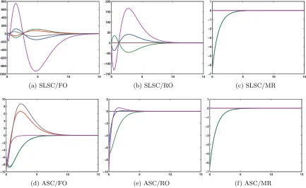
Figure 6.119xe(t)−xb(t) for SLSC/MR, ASC/MR, and LSC/MR observers. (Cf,δ = 0.1,
η = 1000,ξ= 0.1) . . . 181 Figure 6.120The observer differences, SLSC – ASC and SLSC – LSC, confirm the
construction of the MR observer distinguishes between neither completion nor Λ. ex(t)−xb(t) progression inil(t); varyingη affects the MR observer’s
convergence. (Cf, Λ3SL, Λ4A, ΛL,δ= 0.1,ξ = 0.1) . . . 181 Figure 6.121Completion solution and MR observer estimate inil(t) for two examples
Chapter 1
Introduction
The state of a physical system is not always available. Measurements may be hindered by cost or sensor inaccessibility, for example. But in some applications, knowing the state is impor-tant. In [122], Luenberger proposed a method for estimating the state so the estimate in lieu of a true value could be used in a feedback control law. This method designed an observer, which is a system of equations that utilizes the available measurements, or observations, on the inputs and outputs of the physical system to produce an asymptotic estimate of the state. The system of equations is constructed from a mathematical model of the physical system. Initial observer design focused on physical systems described by linear time-invariant systems of ordinary differential equations (ODEs). As research progressed, the systems became more general, incorporating time-varying coefficients and nonlinear structure. Research has also been extended to constructing observers for physical systems described by systems of differential algebraic equations (DAEs), the focus of this dissertation. Since the development of observers to estimate the state for use in a feedback control law, observers have been designed to estimate a system’s unknown parameters [80]; applied to fault estimation, detection, and isolation [103], [117], [171] and disturbance detection [119]; implemented for tracking [162]; and included in power systems [67] and circuit theory [124].
A system F( ˙x(t), x(t), u(t), t) = 0 with a singular ∂F/∂x˙(t) is a system of DAEs. These systems consist of both ODEs and algebraic equations so that ˙x(t) cannot be solved for explicitly. The algebraic equations are identified as explicit constraints but implicit or hidden constraints exist if the index of the system of DAEs is greater than 1 [59]. The index is an identifier of the system of DAEs and two definitions found in [28] are presented.
Definition 1.2. The indexkof a linear system of DAEs E(t) ˙x(t) +F(t)x(t) =B(t)u(t) is the minimum number of times the system is differentiated with respect to t so that the coefficient matricesE(t),F(t)from the derivative array equations E(t)w(t) +F(t)x(t) =B(t)v(t)meet the following conditions:
1. h E(t) F(t)
i
is full row rank for all t;
2. E(t) has constant rank; and
3. if x(t) isn dimensional, thenE(t)b(t) = 0 for some vector b(t) implies the first n entries of b(t) are zero for all t.
Definition 1.2, a specific version of general Definition 1.1, includes checks easily implemented in an index-determining algorithm for a time-invariant system. Note for Definition 1.2, the derivative array equations are revisited in Chapter 2 and conditions 1 and 3 are related to the concept of 1-fullness. These definitions describe what may be clarified in the literature as the differentiation index [47]. Other indices associated with systems of DAEs such as the perturbation index [47], the differential algebraic index [140], the Kronecker index [148], the tractability index [148], or the geometric index [148] are unnecessary for the research in this dissertation; thus, the adjective differentiation is assumed when discussing the index. A system of ODEs is an index 0 system of DAEs, so the higher the index, the greater the challenge is for solving a system of DAEs compared with solving a system of ODEs.
A linear system of DAEs E(t) ˙x(t) +F(t)x(t) = B(t)u(t) is solvable if, given B(t)u(t), the system’s solution is determined by a consistent initial condition [28]. These consistent initial conditions must satisfy all constraints, and if they do not, an incorrect system of DAEs is solved. Due to possibly hidden constraints, consistent initial conditions may not be obvious. Research on methods for finding consistent initial conditions includes [30], [57], [112], and [115], but the examples to which we apply our observer construction approach in Chapters 5 and 6 have consistent initial conditions that can be found by hand. We also assume the linear systems of DAEs are solvable, so methods such as those in [48] or [123] are not required for checking the solvability of a system. Note, if a linear system of DAEs is solvable, then matrix E(t) from the derivative array equations in Definition 1.2 has constant rank even though matrixE(t) may not [56].
Two additional terms in this dissertation that require clarification are smooth and solution manifold. We assume the coefficient matrices of the linear systems of DAEs are smooth, meaning at least as many derivatives exist as are needed. The solution manifold, or the manifold of consistent initial conditions in [35], is characterized by the constraints of the system of DAEs and is where the solutions of a system of DAEs live for a consistent initial condition [41].
Other phrases in the literature synonymous with DAEs are descriptor [78], general or gener-alized state space [76], implicit [5], semistate [131], and singular [116]. This variety in terminol-ogy exists because of separate initial investigations into these systems by different disciplines. Examples of applications involving systems of DAEs include chemistry [33], [164]; circuit the-ory [130], [146]; constrained mechanical systems [21], [81]; gas networks [141] (discrete time and observer consideration); power systems [93]; and robotic motion [131]. Article [36] also provides an example overview on higher index systems of DAEs.
This introduction to systems of DAEs includes the information that is necessary for under-standing the discussion in this dissertation. For those readers interested in learning more about systems of DAEs, suggested references include [6], [28], and [106] and for some earlier material consider [5], [44], [45], and [116].
Observers for linear time-invariant systems of DAEs are numerous. Article [129] designs full-order and reduced-full-order observers for systems in descriptor standard form, a form dependent on the matrix pencil. Another form in [163], [165] from which to construct a reduced-order observer is the generalized staircase form. The authors express concern, though, about the computational efficiency of the algorithms required to transform a linear time-invariant system of DAEs into this special form. The observers in [95] are derived from Luenberger observer theory but the systems to be observed should be in normal form. The construction of the full-order and reduced-order observers in [70] requires the computation of more matrices than the one gain matrix commonly found in the design of observers for linear time-invariant systems of ODEs. The observers in [76] and [78] incorporate singular value decompositions, while article [150] focuses on generalized inverses. Proportional integral observers [169] and functional observers [68] are also proposed.
An observer in [134] applies a reduction algorithm to a linear time-invariant system of DAEs in order to reveal a system that can be observed by a system of ODEs. Our observer construction approach for estimating the state of a linear system of DAEs also constructs an observer for a system of ODEs and utilizes a Luenberger observer (described in Chapter 3). Even though the eigenvalues of a linear time-varying system of ODEs do not provide any indication of the system’s stability [170], eigenvalue placement techniques are used to design the observers in [61], [114], and [120]. The author of [114] writes to improve rather than promote this construction technique since eigenvalue placement is implemented for linear time-varying engineering applications.
The observers for linear time-varying systems of ODEs in [133] are also designed with an eigenvalue placement technique. This article’s approach assumes the system to be observed is lexicographic, meaning the system is observable and has an observability matrix with the same rows linearly independent for all time. Article [132] extends the research in [133] to reduced-order observers, and a lexicographic assumption can also be found in [152]. In response to this restriction, the authors of [62] propose forming an augmented system that is lexicographic when the original one is not. Section 3.1 describes why computing, and thereby constructing an observer dependent on, the observability matrix is avoided for our time-varying observers. An observable assumption is also limiting, commented on by the authors of [94]. Other attempts at generalizing linear time-invariant observer designs for linear time-varying systems of ODEs incorporate canonical forms [149], [151].
Previous work in [18], [19], [56] constructs an observer for linear time-varying systems of DAEs similar to our approach, but our design takes advantage of recent developments in sta-bilized completions. Described in detail in Chapter 2, a completion of a system of DAEs is a system of ODEs and is one of many suggestions on how to solve these systems of differential and algebraic equations.
The research on solving systems of DAEs using iterative methods designed for systems of ODEs, commonly backward difference formulas, is expansive. A first attempt at solving linear time-invariant systems of DAEs iteratively implements a backward Euler method [84], [85], [86]. This method is reconsidered along with other numerical methods in [155]. Index 1 assumptions are required in [32] for an implicit Runge-Kutta method; in [102] to treat the system as a stiff ODE; and in [6], [142] for the computer program DASSL.
for a system that is not initially perturbed, the solution of the system being solved may drift away from the true solution if the constraints characterizing the solution manifold of the system of DAEs are not satisfied. The authors of [8] suggest combining forward Euler discretization with backward Euler stabilization to minimize drift. More recently, three general integrators identified as explicit integration, implicit coordinate partitioning, and index one integration are solved using a Gauss-Newton iteration designed to satisfy any system constraints [55], [58], [173]. Index one integration is modified to become the completion considered in Section 2.3. Other articles on solving systems of DAEs include [72], [91], [143], [144].
Common structural assumptions on a system’s index [37] (and references listed earlier) or on the system being in Hessenberg form (defined in Section 5.1) [39], [40], [66] may simplify the processes for solving linear systems of DAEs but do not lend themselves to developing a general observer. Our observer construction approach constructs observers for linear systems of DAEs using completions, which requires no assumptions on a system’s structure and addresses the constraints concern expressed for systems of DAEs.
Chapter 2
Completions
A completion of an index klinear system of DAEs
E(t) ˙x(t) +F(t)x(t) =B(t)u(t) (2.1)
is a linear system of ODEs
˙
e
x(t) =Ae(t)ex(t) +Be(t)
u(t) ˙
u(t) .. .
u(k)(t)
=Ae(t)xe(t) +Be(t)v(t) (2.2)
designed so the solutions of equation (2.2) contain those of equation (2.1). For ann-dimensional state vector x(t), a linear system of DAEs is defined on the less than n-dimensional solution manifold. Equation (2.2) is described as a completion of (2.1) since it is defined on a complete
n-dimensional space that has the solution manifold as a submanifold [46], [138]. Theory in [46] identifies a general form relating all possible completions of a linear system of DAEs.
The completion evolved from theith order,j-block method ((i, j)-method) presented in [42]. The (i, j)-method uses the expansions from an implicit backward Euler method to assemble a
using a singular Newton method. A noted benefit in [34] of working from the derivative array equations is the derivatives are of the original linear system of DAEs and not of numerically computed values.
Our research focuses on three completions of linear systems of DAEs: the least squares completion (LSC), the stabilized least squares completion (SLSC), and the alternative stabilized completion (ASC). An early article on the least squares completion is [46]. This completion uses a generalized inverse to find the unique minimum norm least squares solution of the derivative array equations. The least squares completion is unique since the solution manifold can be determined from the derivative array equations [46]. A concern of [50] revisited in [138], [139] is that consistent initial conditions may not be enough to keep the numerical solution of the least squares completion from drifting off the solution manifold. The desire is to affect the additional dynamics from completing the manifold so the completion’s solutions satisfy the constraints of the linear system of DAEs and converge to the solution manifold if perturbed. The processes proposed in [138] of finding the least squares completion and an alternative least squares completion are each modified in [139] with stabilized differentiation to produce the stabilized least squares completion and the alternative stabilized completion, respectively.
Section 2.1 details the least squares completion; Section 2.2 describes how the process in Section 2.1 is modified to produce the stabilized least squares completion; and Section 2.3 develops the alternative stabilized completion. Each section’s completion is constructed for a solvable index k linear system of DAEs with an n×1 state vector x(t), a square matrix E(t), and smooth coefficient matrices. This chapter concludes with a discussion in Section 2.4 on the stability of these three completions.
2.1
Least Squares Completion
Three steps are required for finding the least squares completion of the linear system of DAEs, equation (2.1). The first step is to construct the derivative array equations
E(t)w(t) +F(t)x(t) =B(t)v(t). (2.3)
For this completion, the structure of (2.3) consists of
E(t) =
E(t) 0 0 . . .
˙
E(t) +F(t) E(t) 0 . ..
¨
E(t) + 2 ˙F(t) 2 ˙E(t) +F(t) E(t) . .. ..
. ... ... . ..
, B(t) =
B(t) 0 0 . . .
˙
B(t) B(t) 0 . ..
¨
B(t) 2 ˙B(t) B(t) . .. ..
. ... ... . ..
F(t) =
F(t) ˙
F(t) .. .
F(k)(t)
, w(t) =
˙
x(t) ¨
x(t) .. .
x(k+1)(t)
, v(t) =
u(t) ˙
u(t) .. .
u(k)(t)
,
where E(t), B(t) are (k+ 1)×(k+ 1) block matrices and vectors v(t) in equations (2.2) and (2.3) are equal. The first block row of this system is the linear system of DAEs and the sub-sequent block rows are the 1st through kth derivatives of equation (2.1), which are found by differentiating with differential polynomial dtd. Having assumed matricesE(t), F(t), and B(t) from the linear system of DAEs are smooth, matrices E(t), F(t), and B(t) are smooth as well. Additionally, E(t) has constant rank from the solvable system assumption [56].
The second step is to solve for a vector w(t) in the least squares sense using E(t)†, the Moore-Penrose pseudoinverse of E(t):
w(t) =
"
˙
x(t) ∗
#
=−E(t)†F(t)x(t) +E(t)†B(t)v(t). (2.4)
Equation (2.4) is a least squares solution [128] of
E(t)w(t) =E(t)E(t)†(−F(t)x(t) +B(t)v(t)),
which is derived from the derivative array equations,
E(t)w(t) +F(t)x(t) =B(t)v(t)
=⇒ E(t)E(t)†E(t)w(t) =E(t)E(t)†(−F(t)x(t) +B(t)v(t)) =⇒ E(t)w(t) =E(t)E(t)†(−F(t)x(t) +B(t)v(t)).
The final step is to define the completion’s coefficient matricesAe(t) andBe(t) from equation
(2.4). By construction, the first n rows of w(t) equal ˙x(t) from the linear system of DAEs. Therefore, matrix Ae(t) is taken as the firstn rows of −E(t)†F(t) and matrix Be(t) is taken as
the firstnrows ofE(t)†B(t). Both matrices Ae(t) andBe(t) are smooth because they are defined
from smooth matrices; E(t)† is smooth since E(t) is smooth and is assumed to have constant rank [77].
2.2
Stabilized Least Squares Completion
completion, the k derivatives in the derivative array equations come from differentiating the linear system of DAEs using differential polynomial dtd +λ, resulting in
E(t) =
E(t) 0 0 . . .
˙
E(t) +F(t) +λE(t) E(t) 0 . ..
¨
E(t) + 2 ˙F(t) + 2λE˙(t) + 2λF(t) +λ2E(t) 2 ˙E(t) +F(t) + 2λE(t) E(t) . .. .. . ... ... . .. ,
B(t) =
B(t) 0 0 . . .
˙
B(t) +λB(t) B(t) 0 . ..
¨
B(t) + 2λB˙(t) +λ2B(t) 2 ˙B(t) + 2λB(t) B(t) . .. .. . ... ... . .. ,
F(t) =
F(t) ˙
F(t) +λF(t) ¨
F(t) + 2λF˙(t) +λ2F(t) .. .
, w(t) =
˙
x(t) ¨
x(t) .. .
x(k+1)(t)
, v(t) =
u(t) ˙
u(t) .. .
u(k)(t)
. d
dt+λrepresents stabilized differentiation and works to stabilize the additional dynamics of the
completion. Stabilization parameter λis discussed further in Section 2.4.
2.3
Alternative Stabilized Completion
The process for finding the alternative stabilized completion originated with a method from [105] that constructs a canonical form for a linear system of DAEs. Articles [107], [108], and [111] expand on [105], extracting an index 1 linear system of DAEs from a higher index one without altering the system’s solutions. This extraction is motivated by the availability of numerical methods for solving index 1 and not higher index linear systems of DAEs. Reference [106] provides a comprehensive overview of the material in [105], [107], [108], [111].
The first step for finding the alternative stabilized completion of an indexklinear system of DAEs is to construct equation (2.3), the derivative array equations using differential polynomial
d
dt. From this point on, the derivations differ for the linear time-invariant and time-varying cases,
so their developments are presented separately.
2.3.1 Linear Time-Invariant Case
For a linear time-invariant system of DAEs Ex˙(t) +F x(t) =Bu(t), the coefficient matrices of equation (2.3) simplify to
E =
E 0 0 . . .
F E 0 . ..
0 F E . ..
.. . ... ... . ..
, F =
F 0 0 .. .
, B=
B 0 0 . . .
0 B 0 . .. 0 0 B . ..
.. . ... ... . .. .
Following the construction of the derivative array equations, the firstk block rows of matrices E,F, and fv(t) =Bv(t) are denoted by ˜E, ˜F, and ˜fv(t), respectively.
The process continues with the calculation of three orthonormal bases to define matrices
Z2T, T2, and Z1T. Their developments are presented in terms of singular value decompositions to reflect how the bases are calculated in our numerical algorithm. Matrix Z2T is determined such that Z2TE˜ = 0. Since the columns of Z2 form an orthonormal basis for N
˜ ET, ZT
2 is taken as the transpose of the lastkn−r1 columns ofU1 from the singular value decomposition
˜ E =U1
"
(D1)r1×r1 0
0 0
#
V1T. In block column notationZ2T =
h
ZT
2,0 . . . Z2T,k−1
i
, where each
of the k blocks has n columns. Next matrix T2 is determined such that Z2TF˜T2 = 0. The last
n−r2columns ofV2 from the singular value decompositionZ2TF˜ =U2
"
(D2)r
2×r2 0
0 0
#
V2T are
an orthonormal basis forNZ2TF˜and are used to defineT2. Finally, matrixZ1 is defined such that its columns form an orthonormal basis forR(ET2). MatrixZ1T is taken as the transpose of the firstr3columns ofU3from the singular value decompositionET2=U3
"
(D3)r3×r3 0
0 0
#
V3T.
By construction, matrix
"
ZT
1E
Z2T,0F
#
is nonsingular.
Matrices Z2T and Z1T are used to build the (k+ 1)n×(k+ 1)nmatrix
Γ =
Z1T 0κ×kn
Z2T 0d×n
0d×n Z2T
where dis the rank of Z2T, κ=n−d, and Z3T is a kn×(k+ 1)nmatrix selected so that Γ is nonsingular. The block structure
Γ = "
Z1T Z2T,0
# "
0κ×n Z2T,1
#
. . .
"
0κ×n Z2T,k−1
# h 0n×n i " 0d×n Z3T,0(1 :κ)
# "
Z2T,0 Z3T,1(1 :κ)
#
. . .
"
Z2T,k−2 Z3T,k−1(1 :κ)
# "
Z2T,k−1 Z3T,k(1 :κ)
# ∗ ∗ . . . ∗ ∗ .. . ... . . . ... ...
is helpful in the following development, and ∗ is used to designate a term irrelevant to the calculation of the alternative stabilized completion. Multiplying Ew(t) +Fx(t) =fv(t) on the left by Γ produces ΓE =
"
Z1T Z2T,0
#
E+
"
0κ×n Z2T,1
#
F
"
0κ×n Z2T,1
#
E+
"
0κ×n Z2T,2
#
F . . .
"
0κ×n Z2T,k−1
# E+ h 0n×n i F h 0n×n i E " 0d×n ∗ # E+ "
Z2T,0
∗
#
F
"
Z2T,0
∗
#
E+
"
Z2T,1
∗
#
F . . .
"
Z2T,k−2
∗
#
E+
"
Z2T,k−1
∗
#
F
"
Z2T,k−1
∗ # E ∗ ∗ . . . ∗ ∗ .. . ... . . . ... ... ,
which simplifies to
ΓE =
Z1TE 0κ×n . . . 0κ×n 0κ×n
0d×n 0d×n . . . 0d×n 0d×n
Z2T,0F 0d×n . . . 0d×n 0d×n
∗ ∗ . . . ∗ ∗ ; ΓF = "
Z1T Z2T,0
# F " 0d×n ∗ # F ∗ .. . =
Z1TF Z2T,0F
and for f(t) =Bu(t), Γfv(t) = "
Z1T Z2T,0
#
f(t) +
"
0κ×n Z2T,1
#
˙
f(t) +. . .+
"
0κ×n Z2T,k−1
#
f(k−1)(t) +h0n×n
i
f(k)(t)
"
0d×n
∗
#
f(t) +
"
Z2T,0
∗
#
˙
f(t) +. . .+
"
Z2T,k−2
∗
#
f(k−1)(t) +
"
Z2T,k−1
∗
#
f(k)(t)
∗ .. . ,
which simplifies to
Γfv(t) =
ZT
1f(t)
Z2T,0f(t) +Z2T,1f˙(t) +. . .+Z2T,k−1f(k−1)(t)
Z2T,0f˙(t) +. . .+Z2T,k−2f(k−1)(t) +Z2T,k−1f(k)(t) ∗ =
Z1Tf(t)
Z2Tfv˜(t)
Z2T
˜
fv(t)
0 ∗ .
The augmented form of ΓEw(t) =−ΓFx(t) + Γfv(t) is
[ΓEk −ΓF |Γfv(t)] =
Z1TE 0 · · · 0 −Z1TF Z1Tf(t) 0 0 · · · 0 −Z2T,0F Z2Tf˜v(t)
ZT
2,0F 0 · · · 0 0 Z2T
˜
fv(t)
0 ∗ ∗ · · · ∗ ∗ ∗ . (2.5)
The third row in (2.5) equals the first derivative of the second row:
d dt
0 =−Z2T,0F x(t) +Z2Tfv˜(t)
=⇒ Z2T,0Fx˙(t) =Z2T
˜
fv(t)
0
.
If stabilized differentiation is applied to the second row of (2.5) instead,
d
dt +λ
0 =−Z2T,0F x(t) +Z2Tfv˜(t)
=⇒ Z2T,0Fx˙(t) =−λZ2T,0F x(t) +Z2T
˜
fv(t)
0
The augmented form then becomes
Z1TE 0 · · · 0 −Z1TF Z1Tf(t) 0 0 · · · 0 −Z2T,0F Z2Tfv˜(t)
Z2T,0F 0 · · · 0 −λZ2T,0F Z2T
˜
fv(t)
0
+λZ2Tfv˜(t)
∗ ∗ · · · ∗ ∗ ∗ . (2.6)
The first and third rows of (2.6) can be considered together to form the system
"
Z1TE Z2T,0F
#
˙
e
x(t) =−
"
Z1TF λZ2T,0F
# e
x(t) +
Z1Tf(t)
Z2T
˜
fv(t)
0
+λZ2Tfv˜(t)
, (2.7)
from which ˙ex(t) can be solved for explicitly,
˙
e
x(t) =−
"
Z1TE Z2T,0F
#−1"
Z1TF λZ2T,0F
# e
x(t) +
"
Z1TE Z2T,0F
#−1
Z1Tf(t)
Z2T f˜v(t)
0
+λZ2Tf˜v(t)
, (2.8)
since its coefficient matrix in equation (2.7) is nonsingular. Equation (2.8) is the alternative stabilized completion. IfAeis defined as
−
"
Z1TE Z2T,0F
#−1"
Z1TF λZ2T,0F
#
and if Be is defined as
"
Z1TE Z2T,0F
#−1"
Z1TB 0 . . . 0 0
λZ2T,0B Z2T,0+λZ2T,1B . . .
Z2T,k−2+λZ2T,k−1
B Z2T,k−1B
#
,
then equation (2.8) can be written as ˙ex(t) =Aexe(t) +Bve (t).
The derivation of the alternative stabilized completion includes more steps than are required in a numerical algorithm. As with the completions described in Sections 2.1 and 2.2, the process for finding the alternative stabilized completion can be grouped into three steps:
Step 1: Construct the derivative array equations with differential polynomial dtd and denote
the first kblock rows of E andF as ˜E and ˜F, respectively.
Step 2: Define matricesZ2T =
h
Z2T,0 . . . Z2T,k−1
i
(ncolumns per block),T2, andZ1T so the columns ofZ2are an orthonormal basis forN
˜
ET, the columns ofT
Step 3: Calculate the completion’s coefficient matrices AeandBe:
−
"
Z1TE Z2T,0F
#−1"
Z1TF λZ2T,0F
#
,
"
Z1TE Z2T,0F
#−1"
Z1TB 0 . . . 0 0
λZ2T,0B Z2T,0+λZ2T,1
B . . . Z2T,k−2+λZ2T,k−1B Z2T,k−1B
#
.
2.3.2 Linear Time-Varying Case
In Subsection 2.3.1, the alternative stabilized completion was derived from a subsystem of the derivative array equations that did not include the kth derivative of the linear system of DAEs. The information provided by an additional differentiation is superfluous in the linear time-invariant case but necessary in the linear time-varying case.
Following the construction of the derivative array equations, a matrixZ2(t)T is defined such that the columns of Z2(t) form an orthonormal basis forN E(t)T
. Multiplying equation (2.3) on the left byZ2(t)T and then moving all remaining terms to the right-hand side results in
0 =−Z2(t)TF(t)x(t) +Z2(t)TB(t)v(t). (2.9)
Applying stabilized differentiation once to equation (2.9) produces
0 =
d
dt +λ
−Z2(t)TF(t)x(t) +Z2(t)TB(t)v(t)
0 = −Z˙2(t)TF(t)x(t)−Z2(t)TF˙(t)x(t)−Z2(t)TF(t) ˙x(t)−λZ2(t)TF(t)x(t) + Z2(t)TB(t)v(t)0+λZ2(t)TB(t)v(t)
from which
Z2(t)TF(t) ˙x(t) = −
Z2(t)TF(t)
0
+λZ2(t)TF(t)
x(t)
+
Z2(t)TB(t)v(t)0+λZ2(t)TB(t)v(t)
. (2.10)
Next matricesT2(t) andZ1,0(t)T are determined so the columns ofT2(t) are an orthonormal
basis forN Z2(t)TF(t)
and the columns ofZ1,0(t) form an orthonormal basis forR(E(t)T2(t)).
By construction, matrix
"
Z1,0(t)TE(t) Z2(t)TF(t)
#
is nonsingular. Therefore,
considered together with equation (2.10) produces system
"
Z1,0(t)TE(t) Z2(t)TF(t)
#
˙
e
x(t) = −
"
Z1,0(t)TF(t)
Z2(t)TF(t)0+λZ2(t)TF(t)
# e
x(t)
+
"
Z1,0(t)TB(t)u(t)
Z2(t)TB(t)v(t)0+λZ2(t)TB(t)v(t)
#
whence ˙xe(t) can be solved for explicitly. The alternative stabilized completion is
˙
e
x(t) = −
"
Z1,0(t)TE(t)
Z2(t)TF(t)
#−1"
Z1,0(t)TF(t)
Z2(t)TF(t)0+λZ2(t)TF(t)
# e
x(t)
+
"
Z1,0(t)TE(t)
Z2(t)TF(t)
#−1"
Z1,0(t)TB(t)u(t)
Z2(t)TB(t)v(t)
0
+λZ2(t)TB(t)v(t)
#
. (2.11)
The structure of equation (2.11) is reminiscent of ˙xe(t) = Ae(t)xe(t) +Be(t)v(t), but the first
derivative of vectorv(t) keeps a matrix Be(t) from being defined independent of the input u(t)
and its k+ 1 derivatives.
The process of finding the alternative stabilized completion requires the computation of three orthonormal bases to define matrices Z2(t)T, T2(t), and Z1,0(t)T. In a numerical algorithm, a singular value decomposition could be executed at each time t if the bases did not need to be smooth. However, the first derivative of Z2(t)T is required to calculate the alternative stabilized completion. A method presented in [109] and [147] finds a smooth decomposition of a linear time-varying matrix by performing an orthogonal transformation on a non-smooth decomposition. Article [109] also describes a process for determining the first derivatives of the smooth decomposition factors. For convenience, Appendix A includes steps detailing the smooth decomposition and the first derivative definitions.
2.4
Completion Stability
The motivation behind stabilizing the least squares completion and developing the alternative stabilized completion was to improve the stability of the additional dynamics so a completion’s numerical solution would converge to the solution manifold if a perturbation caused drift. The implementation in [139] of stabilized differentiation with differential polynomial dtd +λ
By design, the matrix pencil eigenvalues of a linear time-invariant system of DAEs are also eigenvalues of matrix Ae. A completion’s other eigenvalues come from its additional dynamics
and are referred to as the additional dynamics eigenvalues in this dissertation. If drift occurs but the additional dynamics eigenvalues have a negative real part, the completion’s numerical solution will converge to the solution manifold due to the asymptotically stable additional dynamics. For a constant scalar λ, the additional dynamics eigenvalues equal −λ. Therefore, the desired negative real part results whenλ >0. [137], [139]
If λ = 0, the stabilized least squares completion reduces to the least squares completion and its additional dynamics eigenvalues equal 0. The Jordan canonical form ofAefrom the least
squares completion reveals the 0 eigenvalues are contained in ak×kJordan block. For an index 1 linear time-invariant system of DAEs, the additional dynamics of its least squares completion are stable. Thus, a perturbation’s drift will not grow but the completion’s numerical solution will remain off the solution manifold. For a higher index system, if a perturbation occurs, the resulting drift will grow as linear combinations formed with terms tj, 0 ≤j ≤k−1, from the additional dynamics affect the completion’s numerical solution. Matrix Aefrom the alternative
least squares completion (the alternative stabilized completion when λ = 0) has a different Jordan canonical form. Instead of ak×kJordan block, there is a 1×1 Jordan block for each 0 eigenvalue. No matter the index, the additional dynamics are stable since the only polynomial terms that appear in the linear combinations are constants. Whenλ >0, the linear combinations formed with terms tje−λt for the stabilized least squares completion and with terms e−λt for
the alternative stabilized completion are asymptotically stable. [137], [138], [139]
A completion’s additional dynamics are not well-understood in the time-varying case. Thus, the linear time-invariant system theory acts as guidelines when selecting a large enough constant scalarλ >0 to find a stabilized completion of a linear time-varying system of DAEs [137], [139]. Theory is discussed in [137] for linear time-varying stabilization parameters and remains to be formalized for stabilizing with a matrix instead of a scalar [23].
Chapter 3
Observers
Completions allow us to construct observers for systems of DAEs using design techniques as-sociated with systems of ODEs. The development of the observers being considered assumes a completion of a system of DAEs with output equation has already been found:
˙
e
x(t) = Ae(t)ex(t) +Be(t)v(t) (3.1a)
e
y(t) = C(t)xe(t). (3.1b)
This assumption is necessary in the linear time-varying case to reduce the number of times matrices we construct are differentiated. Additionally, Ae(t),Be(t), and C(t) should be smooth
matrix functions and are assumed bounded. Unless otherwise noted,ex(t) isn×1,ye(t) ism×1,
and C(t) is full row rank.
Section 3.1 describes observability checks for linear systems of ODEs. Sections 3.2 and 3.3 review derivations of a full-order observer and a reduced-order observer, respectively; Section 3.4 presents our observer, the maximally reduced observer; and Section 3.5 introduces the DAE manifold observer for linear time-invariant systems of DAEs. Section 3.6 concludes this chapter by reconsidering completion stability with observability in mind.
3.1
Observable and Detectable
Not every system of ordinary differential equations can be observed. In order for the system to be observable, the information provided through the output needs to make the state distinguishable from the zero solution.
For the linear time-invariant system ˙xe(t) =Aexe(t)+Bve (t) with output equationey(t) =Cxe(t),
O=
C
CAe
.. .
CAen−1
.
The entries of O are the coefficient matrices of ex(t) from ey(t) and its firstn−1 derivatives. If matrixOis full column rank, then the system, as well as the pairA, Ce
, is observable and an observer can be designed to asymptotically estimate the state.
If the rank of O is no < n, the possibility of observing the linear time-invariant
sys-tem becomes dependent on the eigenvalues of Ae. The similarity transformation matrix Q = h
Qno v1 . . . vn−no
i
is assembled from the basis vectors of N(O) ({v1, . . . , vn−no}) and
from no vectors chosen to make Q nonsingular (Qno). Matrices Au =Q
−1
e
AQ =
"
A1 0
A2 A3
#
and Cu =CQ =h C1 0
i
reveal the standard form for the unobservable system. The eigen-values of blockA1are observable, while the eigenvalues of blockA3 are unobservable. Although the unobservable eigenvalues cannot be affected to make the observer converge to the true state, if all eigenvalues of block A3 have a negative real part, then the observer can still be designed to asymptotically estimate the state. These systems for which (A1, C1) is the observable pair and the unobservable eigenvalues are stable (negative real part) are referred to as detectable. IfC1 is not full row rank, it should be redefined with only its linearly independent rows. [4]
It is possible to check the observability of a linear time-varying system of ODEs using the observability matrix [154]. However, for system (3.1) the n−1 derivatives of ye(t) needed to
constructO(t) require knowing the first n−2 derivatives ofAe(t) and the firstn−1 derivatives
of C(t). Unless matrix Ae(t) can be defined symbolically in terms of quantities with known
derivatives, differentiating a computed matrix may introduce numerical error into the observ-ability matrix and possibly produce an incorrect rank. Derivatives of Ae(t) can be computed
using larger derivative arrays, but that approach is not presently considered.
One alternative method for checking the observability of a linear time-varying system of ODEs solves a Lyapunov differential equation
∂Wo(t)
∂t =−Ae(t)
TW
o(t)−Wo(t)Ae(t)−C(t)TC(t) (3.2)
by integrating backwards in time withWo(tf, tf) = 0 [60]. The observability GramianWo(t0, tf) is defined
Wo(t0, tf) =
Z tf
t0
where Φ (t, t0) is the state transition matrix ( ˙Φ (t, t0) =Ae(t)Φ (t, t0) and Φ (t0, t0) = Φ (t0) =I).
The method implemented for the linear time-varying example in Chapter 6 integrates forward in time with Wo(t0, t0) and solves the system
d
dtWo(t) = Φ(t)
TCT(t)C(t)Φ(t) (3.4a) d
dtΦ(t) = Ae(t)Φ(t). (3.4b)
If there exists a time tf such that rank (Wo(t0, tf)) = n for t0 < tf < ∞, then system (3.1)
is observable and
e
A(t), C(t)
is its observable pair [4]. If system (3.1) is not observable, a similarity transformation can also be applied in the linear time-varying case to identify the standard form for the unobservable system. The transformation matrix should be smooth and bounded and have a bounded inverse [160]. As long as these conditions are met, the structure ofQ(t) can remain the same asQwithout having found the observability matrix sinceN(O) =
N(Wo(t0, tf)) [4]. From [159], [160], if the unobservable system ˙x3(t) =A3(t)x3(t) is uniformly asymptotically stable, then system (3.1) is detectable. For our numerical algorithm, a system is detectable if the norm of its unobservable system’s state transition matrix goes to zero as time goes to infinity. An alternative definition for detectable is given in Subsection 3.2.2.
3.2
The Full-Order Observer
The full-order observer ˙
b
x(t) = Ae(t)bx(t) +Be(t)v(t) +L(t) (ye(t)−by(t)) (3.5a)
b
y(t) = C(t)xb(t) (3.5b)
is an example of a Luenberger observer because of its use of known inputs and outputs from the physical system to be observed and because of its assignment of observable eigenvalues to the left half-plane in the linear time-invariant case [121], [122]. Observer (3.5) uses a correction term to compare the plant outputye(t) with the observer outputby(t) (the output resulting from
the observer calculated state). If data exists for the plant output, then these results from the physical system can be substituted into (3.5a) forye(t).
A measure of the observer’s state estimate is e(t) =xe(t)−xb(t), the difference between the solution of the completion and its estimated value. The first derivative of estimation errore(t),
˙
e(t) = xe˙(t)−xb˙(t)
= Ae(t)xe(t) +Be(t)v(t)−
e
A(t)bx(t) +Be(t)v(t) +L(t) (ye(t)−by(t))
= Ae(t) (xe(t)−xb(t))−L(t)C(t) (ex(t)−bx(t))
= Ae(t)−L(t)C(t)