Multi-dimensional Non-linear Response of Steel Frame Structures under Multi-dimensional Ground Motions

Multi-dimensional Non-linear Response of Steel Frame Structures under Multi-

dimensional Ground Motions

Yousuke Murakami ~), Naohiko Tsunashima ~), Noboru Maeda 2), Manabu Endo 3) and Hitoshi Maeno 3)

1) Kansai Electric Power Co., Inc., Japan

2) Newjec.Inc., Japan

3) Obayashi Corporation, Japan

A B S T R A C T

This paper discusses multi-dimensional non-linear responses of steel frame structures where multi-dimensional ground motions are applied. A steel frame structure with large span truss-type beams is modeled, and artificial ground accelerations with numerically clear characteristics are applied.

Multi-dimensional non-linear response analyses are used for this study, where a combined stress condition of the structure is available. As the first step of multi-dimensional study, both model and applied ground motions are restricted to be two-dimensional (2-D), where one horizontal direction and a vertical direction are considered.

Purposes of this study are the followings. Firstly, clarify the non-linear behavior of the steel frame structure under multi-dimensional ground motions. And secondly, study relations between the phase angle of the input motion and non- linear responses of structures.

I N T R O D U C T I O N

For better understanding on seismic responses of structures, a consideration of multi-dimensional components of ground motions is essential. Many studies have been done which were focused on multi-dimensional ground motions and structural responses, and in terms of designing structures within a standard level, combination methods of multi-dimensional components are established such as the square root of sum of square (SRSS) method. Most of these studies were focused on linear or close to linear regions of structures.

On the other hand, recent large earthquakes show that structures may heavily damaged under large multi-dimensional ground motions, and in such cases, structures may behave in non-linear regions. Although some studies have been done, multi-dimensional non-linear responses of structures were still not well known yet.

In this paper, a steel frame structure with large span truss-type beams is modeled, and responses of the structure under multi-dimensional design level and larger input ground motions are studied. A non-linear dynamic analysis method where a combined stress condition of the structure is available may be used for this study. Used ground motions are artificial ground accelerations.

ANALYSIS M O D E L A N D INPUT GROUND M O T I O N S

Analysis Model

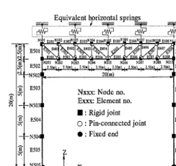
The target structure is a steel frame with large span truss-type beams as a typical example of power station in Japan. Figure 1 shows a schematic view of the steel frame structure.

Equivalent horizontal sprin~s

::Tiiiiiii:i£ iiiiiii:i£ iiii:iii:ii Tiiiii:ii: T:J

--~-N502| ~ 20(m)

--1 E5°3 Nxxx: Node no. F_513 --~-N5031 I Exxx: Element no. N513

I " Rigid joint

_~,[ E504 0 ' Pin-connected joint ~14 ---I-N504 1 O ' Fixed end IN514

__~] E505 ~ E515

• N515

~ ~ x ~ ~

Fig.1 Schematic view of steel frame structures Fig.2 Analysis model

SMiRT 16, Washington DC, August 2001 Paper # 1419

In this study, a single 2D-frame part of the structure, which is shown as bold lines in the Figure 1, is selected and is modeled for a dynamic non-linear analysis. Figure 2 shows the analysis model. This frame model consists of two columns, a truss beam and equivalent horizontal springs. The equivalent horizontal springs are prepared in order to synchronize the horizontal natural period of the model with that of target structure, because without these springs, the 2D-frame model may show much longer natural period in horizontal direction as the result of lack of modeling from the full 3D-frame characteristics. The feet of the model are fixed, where the input ground motions are applied.

As a typical example, horizontal and vertical natural periods are set to be 0.5 second and 0.2 second respectively. The analysis model is tuned to perform these natural periods, also considering that the model adopts typical steel frame members and loading weights. Table 1 shows adopted major parameters in the analysis model.

Tab.1

Member

_{(turn 2)}

Effective area for shear

(mm 2)

Major parameters in the analysis model

Moment of Young's Shear modulus

second order modulus _{(kN/mm 2)}

( m m 4 ) (kN/mm 2)

Column 51,420 216,000 7.04 x 109

Chord 17,190

7,730 5,549 Brace

4,200 3.98 x 108

1,708 6.04 X 107

Strut

205 79

Yield stress (N/mm 2)

325

235

Non-linear characteristics considered in the model follow "Recommendations for the Plastic Design of Steel Structures" established by AIJ (Architectural Institute of Japan). For the members that have pin-connected joints such as struts and braces, a buckling model presented by Wakabayashi [1,2] is used, and for members that have rigid joints such as columns and chords, a plastic-hinge model is used. Table 2, Figure 3 and Figure 4 show the restoring force characteristics of these models. Table 3 shows the characteristics of Wakabayashi model, and Figure 5 shows the moment-axis force interaction curve.

Member

Column Upper chord Lower chord

Tab.2 Bending moment and axial force corresponding to yielding

Bending moment (kNm) Axial force (kN)

Tension Compression Tension Compression

4.56 x 103 4.56 X 103 1.66 X 104 1.09 X 104

5.99 x 102 5.99 x 102 4.09 X 103 4.09 X 103

5.02 x 102 5.02 x 102 4.09 X 103 3.44 X 103

Member

Brace Strut

Tab.3 Characteristics of Wakabayashi model of brace and strut

Moment of second order Buckling

Yield stress (kN) about buckling axis (mm 4) length (mm)

1.81 x 103 5.72 X 106 3536

1.30 x 103 9.84 X 106 2500

M(Bending moment) E:Young's modulus l

I :Moment of inertia / . ~..---~",~, a -- 0.01 MTy[ .. . . ~...,....-..,~,~....

of inertia /

Ko ~ El

i ~ = 0 (End rotation)

O

... Mcr

N(Axiil force)

NTy ' ~ bcr 0 ~ K ° "-E] &

~ ' ] N c r

E:Young's modulus 1 :Length A:Area

ct = 0.01

(Deformation)

(a)

N(Axia~ Force)

pNI{

K1 • Stiffness L

5 (deformation)

N(Axial Force) , , 2

[U_U ° ~2 Mu l Mu + tN-N°~ =1, Mu >0

Mz.

N M

{ / "(Bending

moment)

-N 3

Fig.4 Restoring force characteristics curve of brace and strut

Fig.5 M-N interaction curve

Input Ground Motions

The input ground motions are artificial ground accelerations with numerically clear characteristics. All ground motions have identical Fourier spectrum amplitudes, but have different Fourier spectrum phase angles (the probability density function (PDF) of differences of adjacent phase angles (DAP) is set to be Gaussian). As Watanabe [3] stated, the distribution characteristics of DAP has close correlation to the envelope of the wave. Therefore, the waveform may be statistically controlled by the DAP parameters. Thus, the mean and standard deviation of the Gaussian PDF are selected to be parameters. The waveform ~(t) takes the following forms"

where, A(m i) = 200Ti,

n

~(t) = ~ A(t.oi) cos(t.oit + 0 i ) i=1

T i = 2 a : / m i, (Ti<0.5), A(m i) = 100, (T i > 0.5)

(1)

i 1 ( - ~

0 i = ~AOj, p(A0) = e

j=l 2 ~ 0

(ao-~) 2

202

₍₂₎

Here, m is an angular frequency, A(m) is an amplitude of the sinusoidal wave, 0 is a phase angle, A0 is DAP, p(A0) is PDF of DAP, and ~t and o are mean and standard deviation of the PDF respectively. Fig.6 shows a diagram of input wave generation process. Four different type waveforms are prepared named A, B, C, and D, details of them are shown in Table 4.

00.5 Period

p(AO) ~AO~

~= 0 ... ....,. .... ..:.:

= A0~ ~ ~tlf ~ . = 2 ° :'.<- ~:S"' ~.; .g.

~-, Period T

Phase difference

Gussian distribution of phase difference

0 =Z A0 7g . . ° . ' . . . , %~.. " . . o . ° ° °

¢~ • ° ° . ~ , & . l ~ , ° "

Period T

verse

/

FFT ~ ~ hA ,{~} ,AAAA^^^^^.a.~

Input wave in time domain

Tab.4 Parameters of input waves (Level 2) Group name

A

Parameters controlling the Mean IX

0.5z~

0.5z~

1.0~

1.0~

phase angle of input waves Standard deviation o

0.10~

0.20~

0.30z~

0.40:t

Wave name BH102 BV102 BH103 BV103 BH202 BV202 BH203

Input direction Horizontal

Vertical Horizontal

Vertical Horizontal

Vertical Horizontal

Max. amplitude (cm/s 2) -1008.23

-604.94 -950.69 -570.42 -794.52 -476.71 675.68 BV203

BH302 BV302 BH303 BV303 BH402 BV402 BH403 BV403

Vertical Horizontal

Vertical Horizontal

Vertical Horizontal

Vertical Horizontal

Vertical

405.41 635.60 381.38 803.61 482.15 -655.97 -393.59 -601.27 -360.76

As o increases, the envelope of the wave becomes flat. Typically, flat envelope is considered to be that of ground motions when hypocentral distance is far.

In each group, two waves with different random phase angles but both follow the PDF in Eq.(1) are prepared. These two waves are used for study on correlation of combined two components (horizontal and vertical) in input motions. Namely, using same waves (except in amplitude) for the two components makes correlation coefficient = 1, and using two waves (prepared in each group) makes correlation coefficient =- 0.

The amplitudes of the input motions are set as follows. Firstly, grasp the maximum amplitude of the combined wave that let response level of the frame within linear range and call it Level 1. Then, set the standard input motion amplitude 1.5 times larger than Level 1, and call it Level 2. In these levels, the ratio of the vertical component is set to be 0.6 of that of the horizontal component. Fig.7 shows generated input waveforms.

. o . . . . . .

0 5 10 15 21 25 30 35 ,1) 45

(a) Type A (BH102)

~ 6 m

0 5 10 15 21 25 30 35 40

T m ( ~

(c) Type C (BH302)

~830

0 5 10 15 21 25 30 35

~ ( ~ (b) Type B (BH202)

... r]l'l

I'""

< - ~ D ! i i t ~ t i i i i r r i ~ i I i i i i r i i r

0 5 10 15 2) 25 30 35 40

Tm~(sxnn) (d) Type D (BH402)

ANALYSIS RESULTS

Modal Analysis of the Model

Figure 8 shows natural frequencies and exciting functions in principal modes of the model. The exciting coefficient [~ is set based on a modal shape with maximum amplitude is 1.0.

i

a) 1st mode (f=2.0Hz, [3=1.02) b) 2nd mode (f=4.5Hz, [3=1.26)

Fig.8 Exciting functions and principal modes of the analysis model

Non Linear Response Analysis

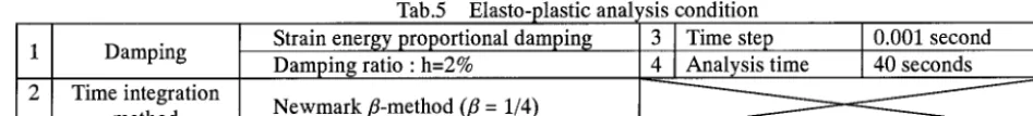
Table 5 shows the conditions of the elasto-plastic analyses. The time increment is set so that the non-linear analyses perform well. Figure 9 shows maximum response forces of the frame compared with that of linear analyses in Type A (case ID = BH102BV102 and BH102BV103), and Type D (case ID = BH402BV402 and BH402BV403). In this figure, a symbol "O" indicates the yielding struts. Figure 10 shows response force orbits in moment-axial force planes at representative columns and chords, and force-deformation relations at representative struts.

1 Damping

2 Time integration

method

Tab.5 Elasto-plastic anal,,sis condition

Strain energy proportional damping 3 Time step 0.001 second

Damping ratio • h=2% 4 Analysis time 40 seconds

Newmark fl-method (/3 = 1/4)

STUDY ON THE ANALYSIS RESULTS

Non-linear Behavior of the Steel Frame Structure under Multi-dimensional Ground Motions

At the level 2 input motion cases, maximum response forces (moment, axial and shear forces) do not differ much by the difference of applied ground motions as shown in Figure 9. The non-linear behavior of the member occurred in only struts at corner regions and it is a buckling (right side of Figure 9).

Due to the developed unbalanced force at the struts, bending moments at some chords nearby are increased as shown in Figure 10-b-2. However, the chords have enough strength and are still in elastic region, and such re-distribution of the response force is observed mostly in local area, not in the whole structure. This trend is universal at any combinations of ground motions within this study.

Relations between the Phase Angle of the Input Motion and Non-linear Responses of Structures

Four different groups of the input motion (A to D, with different DAP) are applied to the model. As stated before, distribution characteristics of DAP has close correlation to the envelope of the wave. As shown in Figure 9 (though in this figure, only A and D are compared, this trend was observed through all groups), different groups may show little difference in the maximum response characteristics. The only differences were numbers and portions of struts which developed a buckling that affects little to whole structures behavior.

Abs. max. value

Member Bending Lo- Axial ., ,

moment(kNm) cation force(kN) memoer

Column 3036 C1 -1892 C2

Uppt~ -229 Ol -1764 02

L~oW~r -341 L1 1855 L2

Brace ~ ~ 1254 B2

~ ~ -1013 , $2

'.1 \ /

/ ~ ~ a l n g m o m

U2 A symbol "(3" indicates the yielding strut.

U2

y

(a) Type A wave (Horizontal:BH102, Vertica "I:BV102, identical phase)

J J1 U2 U ~

L1 L2 '

Abs. max. value Abs. max. value I /

Member _{moment(kNm) cation force(kN)} Bending Lo- Axial

M e m b e r Member Bending Lo- Axial I .. . . I /

. . . m . . . (k~/m) c a t i o n force(~)l ~ m ~ I /

Column 3022 C1 -1287 C2 - - - - Column 2941 C1 -1122 I C2 [---f

Upper chord -229 U1 -1900 U2 U~Ptd 492 U1 -1769 U2

I/

Lower _chord -351 L1 1879 L2 _{L ~ w ~ r - 3 1 1 L 1 1712 L2} [ /

I /

Brace ~ _-.,. ~ 1306 B2 _{Brace ~ ~ 1082 [ B2 t ~}

109 s

s rut

7 7 ; I

/ /

C2

(b) Type A wave (Horizonta "I:BH102, Vertical:BV103, different phase)

U2

x dN J/VVV

Abs. max. value

M e m b e r Bending Lo- Axial moment(kNm) cation force(kN) Member

Column -3411 C1 -1057

Upper

chord -182 U1 -1697

Lower 322 L1 1530

chord

Brace ~ ~ 1048

,Strut ~ -812

C2 U2 L2 B2 $ 2 /

J

/ C1

U2

Abs. max. value

Member Bending Lo- Axial

_ _ Column -3444 C1 -1034

Member moment(kNm) cation force(kN)

C2 Upper

chord -213 U1 -1726 U2

Lower 318 L1 1534 L2

chord

Brace ~ ' ~ , , , , 1030 B2

~ ~ -775 S2,,/

(c) Type D wave (Horizontal:BH402, Vertica "l:BV402, identical phase)

C2

U2

i value

[Member Bending Lo- Axial

moment(kNm) cation force(kN)

Column -3368 C1 -1642

-199 U1 -1641

-332 L1 1625

• _ _ ~ ~ -888

""--\

/

Membez C2 U2 L2 B2 $2

J

/

U2

) M er

~ , Strut ~ ~ -775 $2

(d) Type D wave (Horizontal:BH402 ,Vertical:BV403, different phase)

20 _ 5 ~ 5 4 / ~ 4

~. / \ . . 3 \ . - 3 z - .

~ 1 0 - / " " 2 / ~ 2 ( / \ X~

.~ -5 N / / -2 -1

- \

\ .

. /

",..

/

-10 _ " ~ , / -3

-15 -' ... -5 . . . -4 . . . - 5 - 4 - 3 - 2 - 1 0 1 2 3 4 5

Bending moment M(MNm)

(a-l) Column (E501)

20 15 ~ 10 / ~

o 0 _ \

? - ~ i \

-10 _

/..,,,,,

~f

\

/

-15 ... - 5 - 4 - 3 - 2 - 1 0 1 2 3 4 5

Bending moment M(MNm) (b-l) Column (E501)

400

200 /

0 -200 -400 -600

_

-800 . . . -0.8-0.6-0.4-0.2 o.o 0.2 0.4 0.6 0.8 -0.6 -0.4 -0.2 0 0.2 0.4 0.6 -10 -8 -6 -4 -2 0

Bending moment(MNm) Bending moment(MNm) Deformation (mm) (a-2) Upper chord (El01) (a-3) Lower chord (E201) (a-4) Strut (E401) (a) Type A wave (Horizontal:BH102, Vertical:BV102, identical phase)

5 IBef,)re )'iek ing 3f tte a(tjac

4 I strul(E4~. 3 / " \

'

\

x

0

-1 ~ ~'~ ~"~" ; _{" /} / -2 ~fte~riNel:tine oftae~:tia(ent -3 [s~:ut(li40"]~,.~ / "

-4 ~ , ,

- 5 ...

-0.8-0.6-0.4-0.2 0.0 0.2 0.4 0.6 0.8 Bending moment(MNm)

(b-2) Upper chord (El01)

(b) Ty pe A wave (Horizontal:BH102, Vertical:BV103, different phase)

/ \ ,-,

\

/

"-,, / ~ . , , /

20_ 5

4 15 _ / ' J ' ~

~, / ~ ,_,3 ~ 10 / ' x N 2

--'+9'° 0 " -1

"'~ / / -2

~, -5 \ \ /

-10 ~ , . . / -3

_ ~ f - - 4

-15 ... I -5 - 5 - 4 - 3 - 2 - 1 0 1 2 3 4 5

Bending moment M(MNm) (c-l) Column (E501)

-0.8-0.6-0.4-0.2 0.0 0.2 0.4 0.6 0.8 Bending moment(MNm) (c-2) Upper chord (El01)

i 5 4 lOO_ l

/ ~ o

3 j "

_-

_\

~ ~ ~ - 4 0 0 if" -2 Xx-,,, / -- -600

"-.../ -700 " ~

. . . 800 . . . . . . . . . . . . . . .

-0.6-0.4-0.2 0 0.2 0.4 0.6 -10 -8 -6 -4 -2 0 Bending moment(MNm) Deformation (mm)

(b-3) Lower chord (E201) (b-a) Strut (E401)

5

3

/

,\

2 /

\

1

,.

,,.,

/

3 " ~ / 7

. , 1 . i ... , i , , i , i , , , i i

-0.6-0.4-0.2 0 0.2 0.4 0.6 Bending moment(MNm) (c-3) Lower chord (E201) (c) Type D wave (Horizontal:BH402, Vertical:BV402, identical phase)

100 0

_ -100 ~ - 2 0 0

-300

/

-400

l

-700

-800 . . . -10 -8 -6 -4 -2 0

Deformation (mm) (c-4) Strut (E401)

20,_ 5 - 4 - ~.~ / ~ ~ 3 -

10_ / / " \ 2

" e s (

1

1

0 _ \ . . . / -1

/ -2

~ 5 ~

-10 ~ " - - , , ~ -4

-15 -' ... -5 - 5 - 4 - 3 - 2 - 1 0 1 2 3 4 5

Bending moment M(MNm) (d-l) Column (E501)

5 - 100 -

/ ~ 4 / - ~ o

, I ~ 1 "~ ~ - 3 0 0

-

/

o

400

k,, _1 ~ -500

~,,, / / -2 ~ / -600 / -3 " ~ / - -700

-4 . . . -800 . . . -0.8-0.6-0.4-0.2 0.0 0.2 0.4 0.6 0.8 -0.6 -0.4 -0.2 0 0.2 0.4 0.6 -10 -8 -6 -4 -2 0

Bending moment(MNm) Bending moment(MNm) Deformation (mm) (d-2) Upper chord (El01) (d-3) Lower chord (E201) (d-4) Strut (E401) (d) Type D wave (Horizontal:BH402, Vertical:BV403, different phase)

CONCLUSIONS

1) Within this study model, typical steel flame structure with large span truss-type beams may not collapse by the ground motion level 2 (1.5 times larger than linear limit level).

2) The structure is considered to have almost same maximum response levels when waves normalized to be equivalent linear velocity response are applied, regardless to the DAP characteristics of the wave.

3) Further studies may needed for understanding large deformations due to larger input ground motions, which may hopefully derive ultimate behavior of the structure. In addition, a three-dimensional analysis may be desired for performing the validity of the equivalent horizontal springs in the 2-D model used in this study.

REFERENCES

[1]

[21

[31

Shibata, M., Nakamura, T. and Wakabayashi, M., "Mathematical Expression of Hysteretic Behavior of Braces, Part 1 -

Derivation of hysteresis functions", J. Struct. Constr. Eng., AIJ, No.316, 1982, pp.18-24. ( in Japanese )

Shibata, M. and Wakabayashi, M., "Mathematical Expression of Hysteretic Behavior of Braces, Part 2 -Application to

dynamic response analysis", J. Struct. Constr. Eng., AH, No.320, 1982, pp.29-35. ( in Japanese )

Watanabe, T., Ohsaki, Y., Kanda, J., Iwasaki, R., Masao, T., Kitada, Y. and Sakata, K., "A Study on Generation of Simulated Earthquake Motion, Part IX - Phase Difference Distributions in Narrow Frequency Bands and Envelopes of

Recorded Earthquake Ground Motions", Summaries of Technical Papers of Annual Meeting, AIJ, 1983, pp.685-686.