Activity Recognition from Wireless Sensor
Data
Prashant Dalal 1, Yogesh Kumar 2
M.Tech 4th Semester Student, Department of C.S.E, University Institute of Engineering and Technology,
MDU ROHTAK, Haryana, India1
Assistant Professor, University Institute of Engineering and Technology, MDU ROHTAK, Haryana, India2
ABSTRACT: In this paper, I study the problem of human activity recognition from wireless sensor data. Recent advances in wireless sensor technologies makes this area interesting. I experiment with Naïve Bayes, Markov models and hidden semi-Markov models on three real world datasets [6][4]. The experiments compare different feature representations and different settings of model parameters. Secondly, I focus on the problem of learning from partially annotated training data and need for a querying mechanism to selectively query ’more informative’ training points. I introduce three different active learning schemes based on entropy, mutual information and least margin. I compare these schemes against the random sampling active learning baseline to demonstrate significant gains, specifically for mutual information.
KEYWORDS:Feature representation, Activity learning, Activity recognition, Mutual information, Data labelling.
I. INTRODUCTION
Activity Recognition has become an important technology because of its vast application in real life to human centric problem like healthcare, smart homes play school etc. For example, in mental care hospital, activities of daily living can be used to access the improvement in health of mental patient. Research has been successful in recognizing simple human activities (HA) but recognizing complex HA is an active area of research. Different nature of activities performed and their labelling are some of the challenge.
I experimented with three different models for activity recognition as proposed in [6]. To begin with, I explore the simplistic Naive Bayes model, which does not model any temporal relations between subsequent activities. Naive Bayes model makes the additional assumption that different sensors are independent of each other given the activity. This is followed by the Markov model where each activity represents a state and the sensors are the observations in the standard Markov model framework. However, this model does not model the duration of the activity. Thus, I discuss hidden semi-Markov models, which account for the model duration explicitly.
Datasets
All the experiments in this report have been done on 3 real world datasets. Datasets A and B were introduced in [6] and the third dataset,C is a dataset available on the UCI Machine Learning repository[4]. These datasets involve activities performed by three different people in a house with 3, 2 and 5 rooms respectively. The duration of the datasets is 22 days, 12 days and 21 days respectively, while the number of sensors used is 14,23 and 12 respectively. The annotations were done by the participants using a handwritten diary or a bluetooth headset and the annotations contain a total of 12 activities.
Notation: For each dataset, we are given binary sensor outputs O = {{o11 , o21 ,o31… oN1 },{o12 , o22 ,o32…
of D days. T is dependent on the discretization of time ∆t. The datasets are fully labelled and the activity at time instant t is denoted by yt ∈ {y1 ,y2 ,....yL }.
Feature Representations:∈Three different feature representations were used for our experiments: raw, change-point and last-fired. The observations were first discretized in time and the sensor values were then converted to the feature representations. These feature representations have beenwidely used in past research on the topic.
Raw The raw feature representation lists sets oit to 1 if the sensor i is ON at time instantt. This feature
representation uses all the information that is available, but is noisy in the sense that a sensor might be ON even when it is not being used and thus, can lead to noise in the observations. For instance, the kitchen light may be ON even when the person is not cooking.
Change-point The change-point representation sets oit to 1 if the sensor i switches its state at time instant t.
This feature representation is sparse as compared to raw feature representation. This feature representation is bound to lead to loss of information for models that do not model temporal relations. This is confirmed by the experiments with Naive Bayes approach.
Last Fired The Last Fired representation set the last fired sensor to 1 at each time instant. This representation manages to get rid of raw representation’s noise, while avoiding the constraint of change-point representation.
While all the three feature representations have been used for the experiments in this section, the experiments on active learning have all been done using the Last Fired representation.
II. RELATEDWORK Naive Bayes
The Naive Bayes model does not model any temporal relations. At each time instant t, the vector of sensor values ot is dependent only on the state yt. Further, the Naive Bayes model assumes that the sensors are mutually independent given the activity label, i.e. P(oi, oj|y) = P(oi |y)P(oj y). Learning a Naive Bayes model is straightforward. We just need
to know P(oi |y) for all the sensor, activity pairs. The maximum likelihood solution for this approach is
P(oi |y) =
,
( , )
The model is easy to train and to perform inference, but doesn’t model the underlying distribution well.
Markov Model
The Markov model used for this report is fairly simplistic. Each state represents an activity and the observations correspond to the sensor observations. Staying consistent with the notation described above, each state can take one of the L values and the observation at time step t is the sensor vector ot. We still assume the mutual independence between sensor observations. Given fully labeled data, the transition probabilities aij = P(y(t + 1) = yj |yt = yi) and the emission
probabilities bi(oj) = p(ot = oj |yt = yi) can be learnt in closed form. The closed form solutions is given as:
aij =
, ,
( )
; bi (oj) =
∑ ,
During the inference procedure, we need to find the most probable sequence of states that explains a given set of observations. This can be done by standard dynamic programming methods like the Viterbi algorithm. The fact that the current state is independent of the other states given its previous states makes the inference procedure conducive to a dynamic programming approach.
Hidden Semi-Markov Models
While Markov models described above model the temporal relations in the data, it does not model the duration of a state explicitly. Hidden semi-markov models have been previously proposed in [3] and [6]. This model introduces another variable dt to model the duration of the state at time step t. Learning and inference in semi-markov models is similar to markov models, except that the duration dt is decreased by 1 at every time step and the actual transition in states takes place when dt comes down to zero.
Method
All the experiments were performed on window 7 running machine. Coding was done in Matlab. Three approaches were used leave one out, cross validation and leave two out. Data was collected for three houses A, B and C using sensor introduced in [6]. Sensors used are contact switches to measure open-close states of doors and cupboards; pressure mats to measure sitting on a couch or lying in bed; mercury contacts for movement of objects such as drawers; passive infrared sensors to detect motion in a specific area and float sensors to measure the toilet being flushed[6].
III.EXPERIMENTS
Exemplar based Experiments were conducted with all the three approaches, using different feature representations mentioned above. Accuracy of prediction is listed in tables 1 2 and 3. Different discretizations,_tof the given data were tried. For each run of experiment 1 and 2, one day was left out of the training set to be used as a test set. The reported accuracy results are obtained by averaging over all runs. Two days were left out for 3. Important trends noted in the results was that the standard deviation in accuracy was quite high.
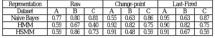
Representation Raw Change-point Last-Fired
Dataset A B C A B C A B C
Naive Bayes 0.77 0.80 0.81 0.55 0.63 0.86 0.95 0.63 0.87 HMM 0.59 0.67 0.40 0.92 0.82 0.75 0.90 0.82 0.75 HSMM 0.59 0.86 0.73 0.91 0.48 0.59 0.91 0.67 0.59
Table 1: Accuracy with ∆t=60 s, Leave one out
Table 1 shows Last fired approach of data representation gives better accuracy then other two with all the models used for activity recognition.
Representation Raw Change-point Last-Fired
Dataset A B C A B C A B C
Naive Bayes 0.81 0.81 0.82 0.77 0.77 0.83 0.85 0.79 0.83 HMM 0.77 0.77 0.49 0.86 0.85 0.65 0.82 0.85 0.66 HSMM 0.79 0.85 0.63 0.86 0.82 0.54 0.82 0.82 0.55
Table 2: Accuracy with t=600 s, Leave one out
Thus, any trend predicted from the data needs to be verified by using larger datasets. Secondly, as described before, Naive Bayes doesn’t perform well using the Change-Point representation as the change point representation is sparse and inherently assumed that the model used for learning takes into account the temporal relations in the data. However, this is not the case when the discretization value used is large. This is because, the change-point representation ceases to be sparse in this case. Thirdly, no clear trend between HMM and HSMM is seen. Fourth, increasing time step size from 60 s to 600 s leads to worse performance in general. This is because the feature representation sometimes throws away important information. To reiterate the most important point, these results highlight the need for larger datasets, which instead calls for reduction in cost of annotating data, which is what we explore in the subsequent section.
IV.ACTIVELEARNING
A key problem in activity recognition is the cost associated in labeling the activities once the data from wireless sensors is received. The above datasets are fairly small and do not generalize well to a different person. Thus, it becomes important to make the participants label data selectively. One possible option is to make the participants label randomly sampled data. Here, we discuss three alternative criteria to the random sampling approach: Entropy, Least Margin and Mutual Information. These active learning criteria have been widely used in past research. However, adapting them to the activity recognition problem is not trivial. First of all, we need a method to train our Markov models from partially labelled data.
Partially Hidden Markov Models
Partially hidden markov models have been discussed previously in research. For this project, I implemented the version described in [5]. For sake of brevity, I would point to the paper for details and give an overview of their approach here. In their framework, some of the states in the HMM (corresponding to activities in our task) have some information revealed about them (which restricts the possible states). To be precise, corresponding to each time step t, the corresponding state yt has a vector σt associated with it, where σt ⊆ {y1 , y2 ,y3……… yL} is the set of values that it can take.
For our case, we restrict ourselves to queries in active learning which reveal the state and hence the σt is either a singleton element, or the entire set Y. A modified form of the Bell-Waunch algorithm (which is an expectation maximisation algorithm) is used for learning the model and Viterbi algorithm is used for inference. In our active learning strategy, we randomly sample an initial set of 4 points on each day, except the test day and train our initial sample on it. We use a discretization of 600 seconds and the Last Fired feature representation for our experiments with different active learning techniques. After the initial set, we use the following active learning strategies to pick one point to be labelled and train on the partially labelled data. This process is continued till 15 percent of the training points is labelled. We report the accuracy averaged over 10 runs with randomly chosen test days.
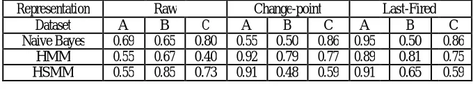
Representation Raw Change-point Last-Fired
Dataset A B C A B C A B C
Naive Bayes 0.69 0.65 0.80 0.55 0.50 0.86 0.95 0.50 0.86 HMM 0.55 0.67 0.40 0.92 0.79 0.77 0.89 0.81 0.75 HSMM 0.55 0.85 0.73 0.91 0.48 0.59 0.91 0.65 0.59
Table 3: Accuracy with t=60 s, Leave two out
From above table, it can be concluded that Last Fired data representation has better accuracy of activity recognition for each probalistic model approach used.
Strategy Random Margin Entropy MI
Dataset A B C A B C A B C A B C
5% 0.63 0.42 0.16 0.62 0.30 0.36 0.57 0.59 0.28 0.75 0.49 0.12 10% 0.73 0.53 0.16 0.74 0.39 0.36 0.59 0.75 0.31 0.89 0.59 0.35 15% 0.74 0.58 0.25 0.77 0.41 0.31 0.61 0.75 0.36 0.89 0.67 0.36 100% 0.82 0.85 0.66 0.82 0.85 0.66 0.82 0.85 0.66 0.82 0.85 0.66
Table 4: Comparison of different active learning methods
From above table it can be concluded that Mutual Information method of activity learning has much better accuracy than all other methods of activity learning prposed. We have achieved better results with lesser amount of data (say) Results achieved with 5% or 10% of data are better or at par with the results achieved with 100% of data. However results for house C are not that good as the person in house C was much inconsistent in his activities.
Least Margin
Least margin,proposed in [1], is simple, but effective active learning technique. It picks the point, about which the existing model is the least confident about, by minimising the margin, defined as Margin(Ot) = P (yt = yi) - P (yt = yj),
where yi and yj are the first and the second most probable labels for the observation at time step t, based on the current
model.
Entropy
Entropy is,intuitively, a measure of randomness or the lack of information about a random variable. Entropy is denoted by H and is defined as H(X) = -∑x p(X = x)log(p(X = x)). In this method, we reveal the state label of the observation
that has the highest entropy, i.e. we reveal the label of the state s = arg maxt(H(yt)).
Mutual Information
Mutual information measures the reduction in entropy over the unlabeled states and is defined as MI(A, B) = H(A)-H(A|B), where H is the entropy. It has been used previously in [2]. For our case, let us denote the unlabeled states by T . We pick the point at time t ∈ T to be labeled, if it is arg maxt∈ T (H(yT \t) H(yT \t|yt))
V. CONCLUSION
We conducted experiments using the setup described above and report accuracies in table 4. It is interesting to note that the experiments give a clear indication that mutual information is a better criterion for active learning point selection. Intuitively, this happens because mutual information takes into account the entropy over the remaining unlabeled samples into account. Secondly, it is clear that the dataset C is harder for these active learning approaches. Third, random sampling baseline is competitive with margin based and entropy based schemes. Another observation worth noting is that the results indicate that significant reduction in training labels is possible.
To conclude, I explored activity recognition for wireless sensors in this report. I experimented with different models for activity recognition on three real world datasets. I also discussed different active learning approaches with an aim towards the reduction of the need of labelled training data.
REFERENCES
[1] B. Anderson and A. Moore. Active learning for hidden markov models: objective functions and algorithms. In ICML, 2005.
[2] A. Krause and C. Guestrin. Nonmyopic active learning of gaussian processes: an exploration-exploitation approach. In ICML, 2007.
[3] K. Murphy. Hidden semi-markov models (hsmms). Technical report, University of British Columbia, 2002.
binary sensors. Sensors, 2013.
[5] T. Scheffer and S. Wrobel. Active learning of partially hidden markov models. In In Proceedings of the ECML/PKDD Workshop on Instance Selection, 2001.