DOI: 10.1534/genetics.105.044099
Conditional Coalescent Trees With Two Mutation Rates and Their
Application to Genomic Instability
Mathieu Emily and Olivier Franc
x
ois
1TIMC–TIMB Department, Faculty of Medicine, Institut de l’Inge´nierie de l’Information de Sante´, 38706 La Tronche, France
Manuscript received April 6, 2005 Accepted for publication December 13, 2005
ABSTRACT
Humans have invested several genes in DNA repair and fidelity replication. To account for the disparity between the rarity of mutations in normal cells and the large number of mutations present in cancer, an hypothesis is that cancer cells must exhibit a mutator phenotype (genomic instability) during tumor progression, with the initiation of abnormal mutation rates caused by the loss of mismatch repair. In this study we introduce a stochastic model of mutation in tumor cells with the aim of estimating the amount of genomic instability due to the alteration of DNA repair genes. Our approach took into account the difficulties generated by sampling within tumoral clones and the fact that these clones must be difficult to isolate. We provide corrections to two classical statistics to obtain unbiased estimators of the raised mutation rate, and we show that large statistical errors may be associated with such estimators. The power of these new statistics to reject genomic instability is assessed and proved to increase with the intensity of mutation rates. In addition, we show that genomic instability cannot be detected unless the raised mu-tation rates exceed the normal rates by a factor of at least 1000.
D
NA replication in normal human cells is an ex-tremely accurate process. During the cell division cycle, copy errors occur with probabilities,109–1010 per nucleotide. In contrast, the malignant cells that constitute cancer tissues are markedly heterogeneous and exhibit alterations in the nucleotide sequence of DNA (e.g., Bielasand Loeb2005). To account for thedisparity between the rarity of mutations in normal cells and the large numbers of mutations present in cancer, Loebet al.(1974) hypothesized that during tumor
pro-gression, cancer cells must exhibit a mutator phenotype
(see the review by Loebet al.2003). It is still a matter of
debate to know exactly which event initiates tumori-genesis. But one hypothesis for the initiation of ab-normal mutation rates in tumors is the loss of mismatch repair (MMR).
For instance, this phenomenon may follow from the inactivation of the genes hMSH2 and hMLH1 involved in hereditary nonpolyposis colorectal cancers (HNPCC) (Fishelet al.1993; Leachet al.1993; Lindblom et al.
1993). In normal conditions, the MMR repair system involves a complex interaction among the protein prod-ucts of hMSH2 and hMLH1 genes. The result is to elim-inate99.9% of the errors in DNA replication, reducing errors to a rate of1/1012bp in genes that regulate the apoptosis or the cell cycle duration. HNPCC is inherited in an autosomal dominant fashion. One copy of the
mutant allele is defective and is inherited in the germ-line. The loss of MMR may start when the second muta-tion occurs somatically as a consequence of the two-hits theory (Moolgavkarand Knudson1981).
Widespread genomic instability seems associated with MMR-defective genes. For example, microsatellite in-stability is associated with HNPCC (Ionov et al.1993;
Peltomakiet al. 1993; Thibodeauet al. 1993).
Detec-tion of DNA instability is therefore a crucial step in view of noninvasive diagnosis of such forms of cancer. Be-cause numerous mutations are required for the full development of cancer, inactivation of caretaker genes can greatly accelerate its development (Kinzler and
Vogelstein2002). For an account of the etiology and
genetic epidemiology of cancer with a statistical per-spective a major review is by Thomas(2004).
This study introduces a two-rates model of DNA mutation based on the infinitely many sites model
(Watterson1975). We consider a sample ofn
sequen-ces taken from a pretumoral tissue and assume that loss of DNA repair has occurred once (and only once) during the history of thensequences tracking back to their most recent common ancestor. We denote the mutational event by the formal symbolD. The eventDis assumed to occur at a very low rated.
The loss of MMR (occurrence of D) may lead to a 10- to 1000-fold increase in the normal mutation rate m0(Bhattacharyyaet al. 1994; Shibataet al.1994).
However, only the sequences that descend fromDare concerned with such an increase in the mutation rate. Because heterogeneity prevails in cancer tissues and 1Corresponding author:TIMC–TIMB Department, Faculty of Medicine,
Institut de l’Inge´nierie de l’Information de Sante´, 38706 La Tronche, France. E-mail: [email protected]
sampling from the tumor is difficult, we assume that an unknown random number of sequences among the sample descend from the mutationD.
The goal of this study is to provide statistical estima-tors for the raised mutation ratem1under the
assump-tion that the normal ratem0is known, but the number
of descendants ofDis unknown. Two classical statistics are studied (see Hartland Clark1997 for a review in
a population genetics context). The first one is the
nucleotide polymorphismcomputed as the average number of segregating sites in the DNA. The second one is the
nucleotide diversitycomputed as the number of pairwise nucleotide differences. Our main contribution is the calculation of corrections to the classical statistics that are needed because the increase in the mutation rate concerns only a random subgenealogy of the sample.
In our study, the clonal evolution of mitotic cell divisions is assumed to be selectively neutral. More precisely, the evolution of the tissue is approximated by a continuous branching process where one cell dies at random after each division (Moran1962). At least in
the early stages of progression toward tumor cells, this model may be consistent with instability theory. Nev-ertheless the assumption of selective neutrality is still a source of controversy. Opponents of Loeb’s theory support the hypothesis that the number of pretumoral cancer cells increases rapidly with time (see Tomlinson et al.1996, 2002; Tomlinsonand Bodmer1999; Sieber et al.2003). An alternative to the approach developed here would therefore include the rapid growth of tumor clones and the selective advantage of pretumoral cells. It is clear that such assumptions complicate the model and its analysis significantly. Although we believe that the recent contributions by Krone and Neuhauser
(1997), Stephensand Donnelly(2003), and Coopand
Griffiths(2004) may allow some progresses in this
re-spect, the selection perspective will not be presented here. Under the neutral assumption, we model the geneal-ogies of DNA sequences using conditional coalescent trees (Wiufand Donnelly1999; Griffithsand Tavare´
2003; Tavare´ 2004). This formalism has been
devel-oped for the primary purpose of estimating the age of an allele (Griffiths and Tavare´ 1998; Stephens
2000). So far, evolutionary models have been introduced for dating the loss of MMR (Tsaoet al.2000; Calabrese et al.2004). Tsaoet al. (2000) observed microsatellite
alleles in noncoding regions, assuming neutrality as well. However, the need for further mathematical studies has been emphasized in a recent review to better understand the influence of existing hypotheses in the evolution of cancer (Michoret al.2004).
In the next section, we define our notation and give an account of the existing results in the theory of con-ditional trees. In addition, we extend many results of the theory to encompass other times or ages useful in the context of genomic instability and describe an efficient way for simulating conditional trees. In nucleotide
polymorphismand nucleotide diversity, we
intro-duce unbiased estimators of the raised mutation rate m1 based on the number of segregating sites and the
number of pairwise differences within the sample. The statistical errors and the power of tests based on these estimators are then compared using Monte Carlo methods.
CONDITIONAL COALESCENT TREES
Model and notations: We consider a sample of n
copies of a gene at a particular DNA locus taken from a pretumoral tissue and assume that the loss of MMR (eventD) occurred once in the sample history. However, the date and place at which this event occurred in the sample genealogy are unknown. Mathematically, we con-sider taking the limit as the rate of occurrencedtends to zero conditional on Dhaving occurred. In further statements the symbol ¼therefore often replaces the limit symbol asdgoes to zero.
The sample is divided into two random complemen-tary subsamplesBandC. The cardinality ofBis a ran-dom variable denoted byB. Given the numberB¼bof sequences inB, the number of sequences inCis thenc¼ nb. As usual, in studies of conditional coalescent trees, the analysis requires two levels of conditioning. At the first level, the sample has the property that all sequences inBare descendants of the particular mutationDwhile none of those in C are. This property is called the
topological eventand is denoted byE. At the second level, we assume that the mutationDarose only once in the history of the sample. We denote this event byM. Con-ditioning onEimpacts the random topology of the tree, while conditioning onMaffects branch lengths. In the terminology of Tavare´ (2004), conditioning onE\M
amounts to considering a unique event polymorphism in the tree. The probability distribution ofBis called the
frequency spectrumand it can be described as
PðB¼bjE\MÞ ¼ 1 bHn1
; b¼1;. . .;n1;
where Hn1 ¼
Pn1
i¼1 1=i denotes the (n 1)th
har-monic number (see Griffithsand Tavare´1998, 2003;
Stephens2000).
Under the neutral hypothesis, we assume that line-ages coalesce at random, and time is rescaled so that the unit of time corresponds toN generations withN the total cell population size (Kingman1982). In this
set-ting, the normal mutation rate is usually rescaled so that u0/2¼2Nm0and the raised mutation rate isu1/2¼2Nm1.
Conditioning onB¼bleads to a model of genealogies that we refer to as theconditional coalescent tree(Wiufand
Donnelly1999; see Figure 1). All subsequent results are
established conditional on the eventE\M, but with the exception of the appendix we omit this condition to
Background results:To state results about conditional coalescence times, some additional results are needed. As much as possible, we use notations similar to those of Wiufand Donnelly(1999) and Tavare´(2004). Forr ¼
1;. . .;b1, we defineJrto be the total number of
an-cestors at the time the subsampleBfirst hasrancestors. This definition implies thatJrranges between (r11) and
(nb1r). In addition, we denote byJ0the number of
ancestors in the sample at the time theBlineages first coalesce with the rest of the sample. This means that we have
1#J0,J1, ,Jb1,Jb[n:
Similarly, we considerKrto be the total number of
an-cestors at the time the subsampleCfirst hasrancestors. We have
K1,K2, ,Kc1,Kc[n;
where the subset B is replaced by C in the previous definition, and theKr’s are complementary to theJr’s in
the set of labels [1,n]. Note that conditional onJ0¼j, we
haveKr¼r for allr, jandj1 1# Kj. To finish, we
denote byJDthe total number of ancestors in the sample at the time the mutationDoccurs. This implies thatJD takes its values between 2 andnb11. A picture of a tree with a summary of notation is displayed in Figure 2. The conditional joint distributions of theJr’s given the
eventsEorE\Mare described in Tavare´(2004, Chap.
8, pp. 106–109), which we refer to when necessary. For example, we easily deduce that
PðJr ¼jr;r ¼1;. . .;b1jJ0 ¼j;E\MÞ
¼ nj1
b1
1
ð1Þ
for allj,j1, ,jb1,n (see Wiufand Donnelly
1999). This result is useful in the nucleotide
di-versity section. Similar properties are stated without
proofs when they are direct consequences of Tavare´’s notations.
Another useful result concerns the number of ances-tors in the sample at the time when the mutation D occurs. Recall that we have
pDk [PðJD¼kjE \MÞ ¼
nk b1
n1
b
ð2Þ
for allk¼2;. . .;nb11.
The age of the mutation D has been studied by
Griffiths and Tavare´ (1998), Wiuf and Donnelly
(1999), and Stephens(2000). Conditional onB¼b, the
expected age is given by
tD¼2 X
nb11 k¼2
nk11
nðk1Þp
D
k: ð3Þ
Griffiths(2003) gave a nicer formula:
tD¼ 2b nb
Xn
j¼b11
1
j:
The distribution of intercoalescence times:In the stan-dard coalescent, the durations X‘that separate coales-cence events backward in time are independent random variables and have exponential distribution of ratel‘¼ ‘(‘1)/2, where‘is the number of ancestors just before the event. Here we recall how the conditioning onB¼b
and the existence of a unique event polymorphismE\M
further modify the shape of the genealogy by lengthen-ing the intercoalescence times.
The next result can be deduced from Griffithsand
Tavare´(1998) or Stephens(2000). Assume that the
mu-tationDhasB¼bdescendants. The joint probability dis-tribution ofðX2;. . .;XnÞconditional on the eventE\M
has density
Figure1.—Conditional coalescent tree withn¼8 leaves.
The mutationDhasB¼4 descendants.
Figure2.—Coalescence levels inBandCwith their
fðx2;. . .;xnÞ ¼
X
nb11 k¼2
pkDlkxk
Yn
‘¼2
f‘ðx‘Þ; ð4Þ
where f‘(x‘) is the probability density function of the exponential distribution of ratel‘.
As a consequence of Equation 4 we have the following result:
Corollary 1. Assume that the mutation D has B ¼ b
descendants. Let‘¼2;. . .;n.Then we have
E½X‘jE \M ¼ ð11p
D
‘Þ=l‘ if ‘#nb11
1=l‘ otherwise: ð5Þ
(
As a consequence of Equation 4, note that conditional on the eventE\MtheX‘’s are no longer independent random variables. However, Equation 4 has the nice interpretation that once we know that the number of ancestors is equal tokat the timeDoccurs, thenXkhas
gammaG(2,lk) distribution, the otherX‘have exponen-tialG(1,l‘) distribution, and the variables are mutually independent. This remark is useful for simulating con-ditional trees given thatB¼b. Our algorithm is as follows:
1. DrawJD ¼ kaccording to the distribution (pkD) for k¼2;. . .;nb11.
2. DrawJ0from the conditional distribution
PðJ0 ¼jjJD¼k;E\MÞ ¼ 2j
kðk1Þ; j ¼k1;. . .;1:
3. Draw an ordered sequence k#J1, ,Jb1,n
uniformly from the set of ordered integral sequences
Ibðk;nÞ ¼ fk#j1, ,jb1,ng.
4. Fill the holes left in [1,n] by theJr’s with theKr’s.
5. Sample Xk from the gamma G(2, lk) distribution;
otherwise, sampleX‘from the exponential distribu-tionG(1,l‘), for‘6¼k.
Testing for the absence ofD:Here we present a brief study of the power of a rather ‘‘abstract’’ test to reject the null hypothesis H0of absence of the mutationDagainst
the alternative hypothesis H1of its existence. The test is
abstract because it assumes the knowledge of the sample genealogy, and the data set consists of all the intercoa-lescence times (Xk). Under the null hypothesis we assume
that the propertyE holds for a specific subsample ofb
sequences. In the alternative hypothesis we assume that the mutationDhasB¼bdescendants as well. The test statistic consists of the ratio of likelihoods that is believed to behave optimally for reasonably large sample sizes. It can be described as
r ¼Lðx;H1Þ Lðx;H0Þ
¼ X
nb11 k¼2
lkpkDxk:
Under H0, we see that this ratio has the same
distribu-tion as a sum of independent exponential random variables of ratesnk¼1/pkD,
Y ¼ X
nb11 k¼2
EðnkÞ; ð6Þ
whereas under H1it is distributed as Yplus a sum of
independent exponential random variables of ratesnk2,
Z ¼Y1 X nb11
k¼2
Eðn2kÞ: ð7Þ
The criterion for rejection isrgreater than the 0.95th percentile from neutral data sets (see Equation 6). The power of the test was studied numerically from 10,000 replicates ofYandZ. We found that the power did not exceed a value close to 0.2 forn¼10, 20, 50, 100, and
bn. For smallerb’s, the lack in power was even more striking. For example, the power dropped to0.1 for
b/n0.5.
Because we assume the ideal knowledge of tree to-pologies and branch lengths, the interest in these power calculations is more theoretical than directed toward applications. However, these results put some limitations on testing for the occurrence of the mutationD. They are evidence that the occurrence ofDalone conveys too little information for being detected by any kind of statistical testing even if the full genealogy were observed. This could be explained that the shapes of such trees do not undergo significant changes under the occurrence ofD.
NUCLEOTIDE POLYMORPHISM
Corrected estimator: We now take account of the mutations that are superimposed on the conditional coalescent trees. Mutations on the tree branches are distributed according to Poisson processes of ratesu0/2
oru1/2, depending on whereDtakes place. Assuming
the infinitely many sites model of the DNA molecule, we introduce an unbiased estimator of u1 based on the
number of segregating sitesS. This variable equals the number of mutations that occurred during the sample history back to the most recent common ancestor of the sample. In the classical coalescent, S has Poisson distribution of parameter Lnu/2, whereu is the
muta-tion rate, and Ln is the length of the genealogy. The
nucleotide polymorphism or Watterson’s estimator is defined as ˆu¼S=Hn1 (Watterson1975). It is an
un-biased estimator ofuwith the property that
Var½ˆu ¼ 1 Hn21
Xn1 i¼1
u2 i21
u i
:
In analogy with the classical approach, we denote by
LnD the length of the genealogy of the full sample and
byLn1 the length of the subgenealogy ofB. Borrowing
the notation from Wiuf and Donnelly (1999), we
also denote byhnthe time separating the root of the
model, the number of segregating sites can be split into two independent terms
S¼S01S1;
whereS1has Poisson distribution of rate (L
n
11h
n)u1/2
andS0has Poisson distribution of rate (L
n
D
Ln1hn)u0/2.
Taking expectations, we obtain the expected number of segregating sites as
E½S ¼Anu01Bnu1;
where
Bn ¼12ðE½Ln11E½hnÞ;
and
An¼12E½LnD Bn:
Accordingly, an unbiased estimator ofu1can be defined
as follows:
u
^1 ¼SAnu0 Bn
:
Table 1 provides numerical values for An and Bn with
sample sizes in the range 5–50. Exact formulas are derived afterward. First, the expectationE[LnD] results
from Corollary 1 as follows:
1 2E½L
D
n ¼Hn11
1
Hn1
Xn1 b¼1
X
nb11 k¼2
pkD bðk1Þ:
Given that the mutationDhasbdescendants (B¼b), the conditional expectations involved in the computation ofAnandBncan be obtained from the results of Wiuf
and Donnelly (1999) and Griffiths and Tavare´
(2003). On the one hand, Griffiths and Tavare´
(2003) proved that
E½L1
njB¼b ¼
X
nb11 j¼2
pjD X n
k¼j11
2
kðk1Þcjk;
where
cjk ¼b ðb1Þ nk nj
ðnkÞ!ðnjb11Þ!
ðnjÞ!ðnkb11Þ!
for j ¼2;. . .;nb11 and k¼j11;. . .;n. On the other hand, Wiufand Donnelly(1999) showed that
E½hnjB¼b ¼2 X
nb11 k¼2
pDk
k; b¼1;. . .; n1:
The values of An and Bn can then be computed by
summing over allb’s.
Statistical errors and power of tests:In the first half of this section, we evaluate the standard deviation (SD) of the estimatoru^1. The exact computation of Var[u^1]
appears intricate enough so that we resort to Monte Carlo methods. In the second half, we evaluate the power of the statisticu^1to reject the hypothesis that the
muta-tion rate increases simultaneously with the occurrence of the mutationD. Simulations were performed using the R statistical programming language (R Development
CoreTeam2004).
Statistical errors: For evaluating statistical errors, the following experimental design was used. The parameter u0was set equal to the valueu0¼1. Roughly, this
cor-responded to a normal mutation rate per mitotic divi-sion of m0 1010, while the total number of cells N
in the tissue approximated 2.5 billion. We considered three different values for the raised mutation rateu1¼
10, 102, 103, and the sample sizes were taken in the rangen¼10–50. Simulations were performed using the method described in the previous section. Table 2 gives the bias and the standard deviation computed over 10,000 replicates. These results confirm that u^1 was
indeed unbiased. Nevertheless, the standard devia-tions were rather high. This could be explained as the
TABLE 1
Correction coefficients foru^1
n 5 10 15 20 25 30 35 40 45 50
An 2.171 2.693 3.024 3.265 3.455 3.612 3.747 3.864 3.967 4.061
Bn 0.595 0.68 0.713 0.732 0.746 0.756 0.764 0.771 0.776 0.781
Numerical values are shown for the correcting coefficientsAnandBnin the statisticu^1¼ ðSAnu0Þ=Bnfor
nin the range 5–50.
TABLE 2
Statistical errors foru^1
u1¼10 u1¼100 u1¼1000
n E SD E SD E SD
10 9.9 12.0 97.4 112.4 947.5 1109.7
20 10.3 12.5 99.7 122.4 991.9 1211.1
30 10.2 12.8 102.9 126.1 1060.3 1286.1
40 10.2 13.2 100.9 128.9 1018.2 1286.2
50 10.4 13.5 102.0 131.7 1045.7 1235.9
empirical distributions exhibited strong positive skew. In addition, most of the error was contributed by a term that seemed proportional tou12. Forn¼20, we adjusted a
regression model of the formanu11bnu12to the variance,
and an almost perfect fit was obtained as Var¼1.47u12
(R2¼0.999,P,1012). Forn¼40, we obtained Var¼ 1.68u12(R2¼0.997,P,1012). Apparently, SDs did not
exhibit a fast decrease as sample sizes increased. This might be due to a strong correlation of data within the subsampleBand to the fact that the most recent ancestor of this subsample is expected to be recent. Note that the shape of the correcting constantBnsuggested a
logarith-mic rate of decrease of errors toward zero.
Power:A fundamental assumption through this work is that the mutationDhas occurred once in the history of the sample. Assuming a normal mutation rateu0, we
report results regarding the power of the test based on u
^1 to reject the null hypothesis of absence ofDagainst the alternative of its existence together with an increase in mutation rateu1.u0. Results foru0¼1 andu1¼10–
103 are given in Table 3. Power values ranged from
0.06 to0.90. Reasonable powers were obtained for u1.103u
0. No significant improvements were observed
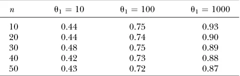
when the sample sizes varied fromn¼10 ton¼50. In a second step we reverted the role of the null and alternative hypotheses and used a test based onu^. The results are reported in Table 4. In this table, powers range from0.43 to0.90. Foru1,10, the test exhibited
per-formances similar to those presented in the previous section where the simultaneous rise in mutation rate was ignored. Significant gains in power were obtained for u1¼103u0. Increasing the sample sizes did not provide
additional benefit. Table 4 indicates that the eventDwas more easily detected when associated with large mutation rates and small sample sizes. However, the power to de-tectDremains small foru1,1000u0.
NUCLEOTIDE DIVERSITY
Corrected estimator:Here we introduce an unbiased estimator ofu1based on the nucleotide diversityP. In
the infinitely many sites model the nucleotide diversity is defined as the mean number of pairwise differences between nucleotides. LetP(i,j) be the number of sites at which the sequenceidiffers from the sequencej, for 1#i#nand 1#j#n. The nucleotide diversity is the average value ofP(i,j). It can be computed as follows:
P¼ 1
nðn1Þ
X
i6¼j
Pði;jÞ:
In the unconditional coalescent, we haveE[P(1, 2)]¼ uE[X2], andPis an unbiased estimator ofu. The
vari-ance ofPis equal to Var[P]¼(n11)u/3(n1)12(n21
n13)u2/9n(n1) (Tajima1983).
Now consider the occurrence ofDand the two rates of mutationu0andu1. Again, we assume that the
muta-tion D hasB ¼b descendants. Consider two arbitrary sequences labeled 1 and 2. In the classical coalescent,
E[X2] is the expected coalescence time of sequences 1
and 2. In analogy with this, the computation ofE[P(1, 2)] requires distinguishing three cases. In the first case, both sequences 1 and 2 belong toB, and we have
E½Pð1;2Þ ¼tBu1;
wheretBis the expected coalescence time withinB. This case occurs with probability (b/n)2. In the second case, one sequence is inBwhile the other belongs toC. This event occurs with probability 2b(nb)/n2, and we have
E½Pð1;2Þ ¼ ð2tB;CtDÞu01tDu1;
wheretB;Cis the expected coalescence time of sequence 1 and sequence 2, andtDis the age ofDgiven in Equa-tion 3. The third case occurs with probability (1b/n)2. It corresponds to the situation where both sequence 1 and sequence 2 are inC. Then we have
E½Pð1;2Þ ¼tCu0;
where tC is the corresponding expected coalescence time. Taking expectation with respect toB, we deduce that
TABLE 3
Powers foru^1
n u1¼10 u1¼100 u1¼1000
10 0.10 0.29 0.90
20 0.06 0.18 0.70
30 0.13 0.29 0.65
40 0.11 0.24 0.59
50 0.09 0.21 0.55
Power of the test based on the statisticu^1is shown, where the null hypothesis H0 is the existence of D and u1 . u0, whereas the alternative hypothesis H1 is the absence of D. The normal rate was set to the valueu0¼1 and the raised rates varied fromu1¼10 tou1¼1000.
TABLE 4
Powers foru^
n u1¼10 u1¼100 u1¼1000
10 0.44 0.75 0.93
20 0.44 0.74 0.90
30 0.48 0.75 0.89
40 0.42 0.73 0.88
50 0.43 0.72 0.87
E½Pð1;2Þ ¼Cnu01Dnu1;
where the constantsCnandDncan be computed from
the above defined coalescence times. Therefore, an un-biased estimatorP1ofu1is of the form
P1¼
PCnu0 Dn
:
Table 5 gives numerical values forCn and Dn forn in
the range 10–50. The next section explains the way the exact computations of all coalescence times can be achieved.
Coalescence times: Here we provide explicit ways of computing the coalescence timestB;tB;C, andtC. As a consequence, we are able to give formal expressions for the correcting constantsCnandDn. Because the formal
expressions are somewhat ugly, the following results should be considered more as recipes for computing expressions than as immediate closed mathematical formulas. The strategy for establishing these exact formulas is rather simple and replicable with slight variations in the three cases.
Case 1—coalescence within B: Let Tj11 ¼Xn1 1 Xj11denote the time at which the sample first hasj
an-cestors. A basic argument shows that if a node has J
ancestors, then its expected age isE[TJ11]. Therefore,
the coalescence time of two individuals in a subsample of sizebfor which the total number of ancestors at each node areJ1, ,Jb1 is given by
tB¼b 11
b1
Xb1 r¼1
2
ðr11Þðr12ÞE½TJr11;
which is made explicit in theappendix.
Case 2—coalescence betweenBandC:The expression of tB;Chas a simple interpretation in terms of the age ofD. The expression given in theappendixcan be reduced,
using a symbolic computing language such as Maple. Because the gamma distributionG(2,lk) is the sum of
two independent exponentials, we find that the co-alescence timetB;C ¼tD(age ofD) plus the coalescence time of two ancestors among the k present at the occurrence ofD. According to Equation 4, the second coalescence time has exponentialG(1, 1) distribution. Hence, we have
tB;C ¼11tD:
Case 3—coalescence withinC:The average coalescence time for two individuals withinCcan be obtained from conditioning onJ0¼jand from the observation that we
have Kr ¼rfor r ,j given thatJ0¼j. This leads to a
complicated formula that uses a series of probabilistic results stated in Lemmas 3 and 4 (see theappendix).
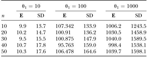
Statistical errors and power of tests:Here we report numerical estimates of the standard deviations of P1,
and we study the power of this statistic to reject the hypothesis that the mutation rate increased simulta-neously with the occurrence of the mutation D. The same experimental design was used as for the statisticu^1
defined in the previous section. The results are closely parallel to those obtained foru^1(see Tables 6–8 ). The
estimator appears to be unbiased. The standard devia-tions are of the same order as those computed for u^1
although they seem slightly higher. UsingP1instead of u
^
1to reject the existence ofDleads to a 12 or 13% loss in
power when u1 ¼100 or u1 ¼103. Reverting the two
hypotheses and using Pyield the same conclusions as for ˆu.
DISCUSSION
Genetic information must be tightly regulated, and its faithful replication and repair is the greatest imperative. To this end humans have invested.130 genes in DNA repair, and this number is even greater if genes dedi-cated to fidelity of replication are included (Anderson
2001; Wood 2001). In this article we introduced a
TABLE 5
Correction coefficients forP1
n 5 10 15 20 25 30 35 40 45 50
Cn 0.996 1.019 1.021 1.02 1.02 1.019 1.019 1.018 1.018 1.018
Dn 0.253 0.218 0.199 0.187 0.178 0.171 0.166 0.161 0.156 0.154
Numerical values are shown for the correcting coefficientsCnandDnin the statisticP1¼(PCnu0)/Dnfor
nin the range 5–50.
TABLE 6
Statistical errors forP1
u1¼10 u1¼100 u1¼1000
n E SD E SD E SD
10 9.9 13.7 107.342 133.9 1006.2 1243.5
20 10.2 14.7 100.91 136.2 1030.5 1458.9
30 9.5 15.5 100.875 147.9 1040.0 1589.5
40 10.7 17.8 95.763 159.0 998.4 1538.1
50 10.3 17.6 106.478 164.6 1039.7 1598.1
stochastic model of mutation in tumor cells with the aim of estimating the amount of genomic instability in cancer tissues due to the alteration of DNA repair genes. Our approach took into account the difficulties gener-ated by sampling within tumoral clones and the fact that these clones must be difficult to isolate (Andersonet al.
2001). We provided unbiased estimators of the normal-ized raised mutation rates. These quantities can be interpreted as the mean numbers of new mutations present in daughter cells after each mitotic generation (this corresponds to an evaluation ofu1/2¼2m1N). The
power of these statistics to reject genomic instability was assessed and proved to increase with the intensity of mutation. However, we showed that large statistical errors may be associated with such estimates. Condi-tional on the presence of loss of MMR within a sample of cells, no significant benefit would be expected from large sample sizes. In addition, we proved that geno-mic instability can hardly be detected unless the raised mutation rates exceed the normal rates by a factor.103. These results suggest monitoring several loci to increase power and reliability of tests and give theoretical support to foundations of current clinical guidelines (Bolandet al.1998).
Computations were conducted under the assump-tions of selective neutrality. Tumors of clonal origin have
long life spans with evolutionary history that may last over 10 or 20 years and exhibits multistep progression. At least in the early stages of tumor progression selective neutrality is still compatible with Loeb’s theory of carcinogenesis. Evidence is lacking that the initiating events are neither highly advantageous nor highly deleterious. A competing assumption explains that a cell must exhibit a selective advantage to be converted into a pretumoral cell. Then by a selective clonal expansion the cell becomes malignant (Cairns 1975;
Nowell 1976; Tomlinsonet al. 1996). The material
presented in this article may serve as a basis for testing such kinds of assumption. A classical way of doing so is by computing Tajima’sD-statistic (Tajima 1989). In
our framework this statistic can be defined as the differ-enceu^1P1. To apply the test,P-values can be obtained
from Monte Carlo replicates, using the new simulation procedure described inconditional coalescent trees.
Genomic instability particularly affects DNA repeat sequences. It has even been calculated to affect hundred of thousands of such sequences in each tumor cell but very few of these events are within coding sequences
(Perucho 1996). It is widely argued that stepwise
mutation models might be more appropriate for such DNA sequences than the infinitely many sites model used in this work. However, genomic instability is not restricted to repeat sequences and even not limited to the nucleus. Mitochondrial DNA may also be mutated in a process that involves clonal expansion (Polyaket al.
1998). Infinitely many sites models may thus be accept-able in several situations.
Anderson et al. (2001) reported several difficulties
with measuring the amount of instability in cancer cell genomes. The ideal measurement would be how many genomic events occur per cell generation because this number would allow evaluation of the rate of tumor progression. Regardless of the fact that it is as yet difficult to approach in clinical application, a rigorous way of calculating unbiased estimates of the amount of genomic instability in pretumoral tissues would never-theless require the correction coefficients described in this article.
The authors thank Robert C. Griffiths for useful discussions about the model and an anonymous referee for correcting some biblio-graphical mistakes. This work is partly supported by a grant from the Algorithmes et Populations Biologiques project, which is supported by the Institut d’Informatique et de Mathe´matiques Applique´es de Grenoble.
LITERATURE CITED
Anderson, G. R., 2001 Genomic instability in cancer. Curr. Sci.81:
501–507.
Anderson, G. R., D. L. Stolerand B. M. Brenner, 2001 Cancer:
the evolved consequence of a destabilized genome. BioEssays 23:1037–1046.
Bhattacharyya, N. P., A. Skandalis, A. Ganesh, J. Grodenand
M. Meuth, 1994 Mutator phenotypes in human colorectal
car-cinoma cell lines. Proc. Natl. Acad. Sci. USA91:6319–6323.
TABLE 7
Powers forP1
n u1¼10 u1¼100 u1¼1000
10 0.09 0.32 0.72
20 0.12 0.29 0.54
30 0.14 0.24 0.44
40 0.12 0.19 0.35
50 0.13 0.20 0.40
Power of the test based on the statisticP1is shown, where the null hypothesis H0 is the existence of D and u1 . u0, whereas the alternative hypothesis H1 is the absence of D. The normal rate was set to the valueu0¼1 and the raised rates varied fromu1¼10 tou1¼1000.
TABLE 8
Powers forP
n u1¼10 u1¼100 u1¼1000
10 0.44 0.73 0.91
20 0.44 0.69 0.84
30 0.39 0.64 0.80
40 0.34 0.64 0.79
50 0.34 0.62 0.76
Bielas, J. H., and L. A. Loeb, 2005 Mutator phenotype in cancer:
timing and perspectives. Environ. Mol. Mutagen.45:143–149. Boland, C. R., S. N. Thibodeau, S. R. Hamilton, D. Sidransky, J. R.
Eshlemanet al., 1998 A National Cancer Institute workshop on
microsatellite instability for cancer detection and familial predis-position: development of international criteria for the determi-nation of microsatellite instability in colorectal cancer. Cancer Res.58:5248–5257.
Cairns, J., 1975 Mutation selection and the natural history of
can-cer. Nature255:197–200.
Calabrese, P., J. P. Tsao, Y. Yatabe, R. Salovaara, J. P. Mecklinet al.,
2004 Colorectal pretumor progression before and after DNA mismatch repair. Am. J. Pathol.164:1447–1453.
Coop, G., and R. C. Griffiths, 2004 Ancestral inference on gene
trees under selection. Theor. Popul. Biol.66:219–232. Fishel, R., M. K. Lescoe, M. R. Rao, N. G. Copeland, N. A. Jenkins
et al., 1993 The human mutator gene homolog MSH2 and its association with hereditary nonpolyposis colorectal cancer. Cell 75:1027–1038 (erratum: Cell77:167).
Griffiths, R. C., 2003 The frequency spectrum of a mutation, and
its age, in a general diffusion model. Theor. Popul. Biol.64:241– 251.
Griffiths, R. C., and S. Tavare´, 1998 The age of a mutation in a
general coalescent tree. Stoch. Models14:273–295.
Griffiths, R. C., and S. Tavare´, 2003 The genealogy of a neutral
mutation, pp. 393–412 inHighly Structured Stochastic Systems, edi-ted by P. Green, N. Hjortand S. Richardson. Oxford
Univer-sity Press, Oxford.
Hartl, D., and A. Clark, 1997 Principles of Population Genetics, Ed. 3.
Sinauer Associates, Sunderland, MA.
Ionov, Y., M. A. Peinado, S. Malkhosyan, D. Shibata and M.
Perucho, 1993 Ubiquitous somatic mutations in simple
re-peated sequences reveal a new mechanism for colonic carcino-genesis. Nature363:558–561.
Kingman, J. F. C., 1982 The coalescent. Stoch. Proc. Appl.13:235–248.
Kinzler, K. W., and B. Vogelstein, 2002 Familial cancer
syn-dromes: the role of caretakers and gatekeepers, pp. 209–210 in
The Genetic Basis of Human Cancer, Ed. 2, edited by B. Vogelstein
and K. W. Kinzler. McGraw-Hill, New York.
Krone, S. M., and C. Neuhauser, 1997 Ancestral process with
selec-tion. Theor. Popul. Biol.51:210–237.
Leach, F. S., N. C. Nicolaides, N. Papdopulos, B. Liu, J. Jenet al.,
1993 Mutations of a mutS homolog in hereditary nonpolyposis colorectal cancer. Cell75:1215–1225.
Lindblom, A., P. Tannergard, B. Wereliusand M. Nordenskjold,
1993 Genetic mapping of a second locus predisposing to hered-itary non-polyposis colon cancer. Nat. Genet.5:279–282. Loeb, L. A., B. N. Springgateand N. Battula, 1974 Errors in DNA
replication as a basis of malignant changes. Cancer Res.34:2311– 2321.
Loeb, L. A., K. R. Loeband J. P. Anderson, 2003 Multiple mutations
and cancer. Proc. Natl. Acad. Sci. USA100:776–781.
Michor, F., Y. Iwasaand M. A. Nowak, 2004 Dynamics of cancer
progression. Nat. Rev. Cancer4:197–205.
Moolgavkar, S. H., and A. G. Knudson, Jr., 1981 Mutation and
cancer: a model for human carcinogenesis. J. Natl. Cancer Inst. 66:1037–1052.
Moran, P. A. P., 1962 The Statistical Process of Evolutionary Theory.
Clarendon Press, Oxford.
Nowell, P. C., 1976 The clonal evolution of tumor cell populations.
Science194:23–28.
Peltomaki, P., L. Aaltonen, P. Sistonen, L. Pylkkanen, J. P.
Mecklinet al., 1993 Genetic mapping of a locus predisposing
to human colorectal cancer. Science260:751–752.
Perucho, M., 1996 Cancer of the microsatellite mutator phenotype.
J. Biol. Chem.377:675–684.
Polyak, K., Y. Li, H. Zhu, C. Lengauer, J. K. Willson et al.,
1998 Somatic mutations of the mitochondrial genome in hu-man colorectal tumours. Nat. Genet.20:291–293.
R DevelopmentCoreTeam, 2004 R: A Language and Development for
Statistical Computing. R Foundation for Statistical Computing, Vienna, Austria. (http://www.R-project.org).
Sieber, O. M., K. Heinimanand I. P. M. Tomlinson, 2003 Genomic
instability—the engine of tumorigenesis? Nat. Rev. Cancer 3: 701–708.
Shibata, D., M. A. Peinado, Y. Ionov, S. Malkhosyan and M.
Perucho, 1994 Genomic instability in repeated sequences is
an early somatic event in colorectal tumorigenesis that persists after transformation. Nat. Genet.6:273–281.
Stephens, M., 2000 Times on tree, and the age of an allele. Theor.
Popul. Biol.57:109–119.
Stephens, M., and P. Donnelly, 2003 Ancestral inference in
pop-ulation genetics with selection. Aust. N. Z. J. Stat.45:395–430. Tajima, F., 1983 Evolutionary relationship of DNA sequences in
finite populations. Genetics105:437–460.
Tajima, F., 1989 Statistical method for testing the neutral mutation
hypothesis by DNA polymorphism. Genetics123:585–595. Tavare´, S., 2004 Ancestral inference in population genetics, pp. 1–
188 inLectures on Probability Theory and Statistics. Ecole d’Ete´ de Prob-abilite´ de St Flour XXXI–2001, edited by J. Picard. Springer Verlag,
New York.
Thibodeau, S. N., G. Brenand D. Schaid, 1993 Microsatellite
insta-bility in cancer of the proximal colon. Science260:816–819. Thomas, D. C., 2004 Statistical Methods in Genetic Epidemiology.
Oxford University Press, New York.
Tomlinson, I. P. M., and W. Bodmer, 1999 Selection, the mutation
rate and cancer: ensuring that the tail does not wag the dog. Nat. Med.5:11–12.
Tomlinson, I. P. M., M. Novelliand W. Bodmer, 1996 The
muta-tion rate and cancer. Proc. Natl. Acad. Sci. USA93:14800–14803. Tomlinson, I. P. M., P. Sasieniand W. Bodmer, 2002 How many
mutations in a cancer? Am. J. Pathol.160:755–758.
Tsao, J. L., Y. Yatabe, R. Salovaara, H. J. Ja¨ rvinen, J. P. Mecklin
et al., 2000 Genetic reconstruction of individual colorectal tu-mor histories. Proc. Natl. Acad. Sci. USA97:1236–1241. Watterson, G. A., 1975 On the number of segregating sites in
ge-netical models without recombination. Theor. Popul. Biol. 2: 256–276.
Wiuf, C., and P. Donnelly, 1999 Conditional genealogies and the
age of a neutral mutant. Theor. Popul. Biol.56:183–201. Wood, A., 2001 Racial differences in the response to drugs—
pointers to genetic differences. N. Engl. J. Med.344:1393–1395.
Communicating editor: M. Nordborg
APPENDIX
Proof of Corollary1. Letn$2. Assuming thatDhasbdescendants (1#b#n1) and using Equation 4 we obtain the marginal distribution of each intercoalescence time. For‘¼2;. . .;nwe have
fðx‘Þ ¼ X nb11 k¼2;k6¼‘
pkD1pD‘l‘x‘
!
f‘ðx‘Þ
if‘#nb11; otherwise, it is
wheref‘is the density of the exponentialG(1,l‘) distribution. Taking expectations it becomes
E½X‘jE\M ¼ ð11p
D
‘Þ=l‘ if ‘#nb11
1=l‘ otherwise:
Lemma1.Let n$2.We have
1 2E½L
D
n ¼Hn11
1
Hn1
X
n1 b¼1
X
nb11 k¼2
pkD bðk1Þ:
Proof.Letb ¼1;. . .;n1. From Corollary 1 we have
E½LD
njB¼b ¼
Xn
k¼2
kE½Xk ¼2Hn112
X
nb11 k¼2
pkD k1:
Then
E½LD
n ¼
Xn1 b¼1
1
bHn1 E½LD
njB¼b ¼2 Hn11
1
Hn1
Xn1 b¼1
X
nb11 k¼2
pkD bðk1Þ
!
:
Lemma2.Let n$2and assume thatDhas b descendants. Let r ¼1;. . .;b1 and k2[2,nb11].For j2[k1r1,n b1r],we have
PðJr¼jjJD¼k;E\MÞ ¼
jk r1
nj1
br1
nk b1
:
Proof.Letk2[2,nb11] andr2[1,b1]. For allj2[k1r1,nb1r] it is known that fork#j1, ,jr1,j
we have
PðJ1¼j1;. . .;Jr1¼jr1;Jr ¼jjJD¼k;E\MÞ ¼
nj1
br1
nk b1
1
(Tavare´2004). Note that the above formula is independent ofj1;. . .;jr1. We have
PðJr ¼jjJD¼k;E \MÞ ¼
X
k#j1,,jr1,j
PðJ1¼j1;. . .;Jr1¼jr1;Jr ¼jjJD¼k;E\MÞ
¼ jk r1
nj1
br1
nk
b1
1
:
Lemma3.Let n$2and assume thatDhas b descendants. Let J0be defined as inconditional coalescent trees. For j¼
1,. . .,nb,we have
PðJ0¼jjE\MÞ ¼2j
X
nb11 k¼j11
pkD kðk1Þ:
Proof.Due to a straightforward combinatorial argument, forj¼1,. . .,nbwe have
n
n
PðJ0¼jjJD¼k;E\MÞ ¼ 2j kðk1Þ:
Then intregrating overJD’s implies that
PðJ0 ¼jjE\MÞ ¼2j
X
nb11 k¼j11
pkD
kðk1Þ; k¼j11;. . .;nb11:
Lemma4.Let n$2,assume thatDhas b descendants,and denote c¼nb. Let r¼j;. . .;c1and Krbe defined as in
conditional coalescent trees. For k2[r11,r1b],we have
PðKr ¼kjJ0¼j;E\MÞ ¼
kj1
rj
nk1
cr 1
nj1
b
:
Proof.Note that the vectorðJ0;. . .;Jb1;K0;. . .;Kc1Þis obtained from a permutation of the labelsð1;2;. . .;n1Þ,
where Jr’s and Kr’s are defined as in conditional coalescent trees. Conditional on J0 ¼ j, the vector ðJ1;. . .;Jb1;Kj;. . .;Kc1Þis also a permutation of the labelsðj11;. . .;n1Þ. Then Equation 1 implies that for j,kj, ,kc1,n, we have
PðKr ¼kr; r¼1;. . .;c1jJ0¼j;E\MÞ ¼
nj1
b
1
:
Note that the above formula is independent ofk1;. . .;kc1. We have
PðKr ¼kjJ0¼j;E\MÞ ¼
X
j,kj,,kr1,r
X
r,kr11,,kc1,n
PðKr ¼kr;r ¼1;. . .;c1jJ0¼j;E\MÞ
¼
kj1
rj
nk1
cr1
nj1
b
:
An explicit formula fortBdefined innucleotide diversityis given by
tB¼ b 11
b1
Xb1 r¼1
2
ðr11Þðr12Þ
X
nb11 k¼2
Xc1r
j¼k1r1
PðJr ¼jjJD¼kÞE½Tj11jJD¼kpkD:
In this expression, we used Corollary 1,
E½Tj11jJD¼k ¼
2ðnjÞ
jn ; forj $k;
and the result stated in Lemma 2 (appendix).
The average coalescence time for two sequences, one within B and one within C, is straightforward from the conditioning onJD. We obtain that
tB;C¼2
X
nb11 k¼2
ðk11Þ
ðk1Þfðn;kÞp
D
k;
where
fðn;kÞ ¼X k
j¼2
E½TjjJD¼k=jðj11Þ; k¼2;. . .;nb11:
Becausej#kin the above summation, we obtain from Corollary 1 that
E½TjjJD¼k ¼
2ðnj11Þ ðj1Þn 1
2
kðk1Þ:
RegardingtC, we have
tC¼2 ðc11Þ ðc1Þ
Xc1 r¼1
E½TKr11
ðr11Þðr12Þ; r ¼1;. . .;c1:
Now we use the fact
E½TKr11 ¼
Xc
j¼1
E½TKr11jJ0 ¼jPðJ0 ¼jÞ:
Forj¼1;. . .;candr,j, we have
E½TKr11jJ0¼j ¼
2ðnrÞ rn 1ej;
with
ej ¼
X
nb11 ‘¼j11
2
‘ð‘1ÞPðJD¼‘jJ0¼jÞ:
Otherwise, we haver$jand
E½TKr11jJ0¼j ¼
Xb1r
k¼r11
PðKr ¼kjJ0 ¼jÞ
2ðnkÞ nk 1ejk
;
where
ejk ¼ X k
‘¼j11
2
‘ð‘1ÞPðJD¼‘jJ0¼jÞ; k¼r11;. . .; b1r: