Inference on Recombination and Block Structure Using Unphased Data
Carsten Wiuf
1Bioinformatics Research Center, University of Aarhus, 8000 Aarhus C, Denmark
Manuscript received December 16, 2002 Accepted for publication September 24, 2003
ABSTRACT
In this study compatibility with a tree for unphased genotype data is discussed. If the data are compatible with a tree, the data are consistent with an assumption of no recombination in its evolutionary history. Further, it is said that there is a solution to theperfect phylogeny problem;i.e., for each individual a pair of haplotypes can be defined and the set of all haplotypes can be explained without invoking recombination. A new algorithm to decide whether or not a sample is compatible with a tree is derived. The new algorithm relies on an equivalence relation between sites that mutually determine the phase of each other. (The previous algorithm was based on advanced graph theoretical tools.) The equivalence relation is used to derive the number of solutions to theperfect phylogeny problem. Further, a series of statistics,RjM,jⱖ2, are defined. These can be used to detect recombination events in the sample’s history and to divide the sample into regions that are compatible with a tree. The new statistics are applied to real data from human genes. The results from this application are discussed with reference to recent suggestions that recombination in the human genome is highly heterogeneous.
C
URRENT efforts, initiated by the National Human Genome Research Institute (http://www.genome.Individual 1: 2 2 Individual 2: 0 0 Individual 3: 1 1 gov), seek to accomplish a haplotype map of the human
genome. One idea underlying these efforts is that
re-Here 0 and 1 denote that an individual is homozygous combination in the human genome happens mainly
for the 0 and 1 allele, respectively, and 2 denotes that in localized regions, so-called hotspots, with little or
an individual is heterozygous. Depending on how the virtually no recombination going on between the
hot-phase of the double heterozygote, 2 2, is assigned, the spots (e.g.,Gabrielet al.2002, and references therein).
inferred haplotypes are indicative of recombination (or This suggests a block-structured genome, where markers
gene conversion) in the sample’s history or consistent within the same block preferentially are inherited
to-with an assumption of no recombination. The presence gether. In consequence, one should be able to infer the
of the four possible gametes in two sites is taken as evidence location of hotspots (or, equivalently the boundaries of
of recombination (cf.the four-gamete test;Hudsonand the nonrecombining blocks) from a detailed map of
Kaplan1985), which is a reliable indicator as long as markers,e.g., single-nucleotide polymorphisms (SNPs),
recurrent mutations are rare or absent. In the following spread throughout the genome. This has been
at-all mutation events are assumed to be unique. tempted by various groups; among these areDalyet al.
Recently,Gusfield(2002) showed that it can be de-(2001), Jeffreys et al. (2001), Johnson et al. (2001),
termined efficiently whether a sample of unphased ge-andGabrielet al.(2002). Unfortunately, when markers
notypes (e.g., the example given above) is consistent are spread with long distances between them, it is
experi-with the assumption of no recombination. If it is consis-mentally difficult and time-consuming to obtain
infor-tent, then the sample is said to be compatible with a mation about phase, i.e., whether a marker allele has
tree: A pair of haplotypes can be defined for each indi-paternal or maternal origin. One must then rely on
vidual and the genealogical history of all these haplo-unphased data. Unphased data, in contrast to phased
types can be illustrated with a tree. It is said that there data, contains less information about the evolutionary
is a solution to theperfect phylogeny haplotype(PPH) prob-history of a sample and increases the risk of inferring
lem (Gusfield 2002, and references therein). Poten-nonexisting hotspots or, oppositely, failing to infer
exist-tially pairs of haplotypes can be defined in various ways ing hotspots and actual recombination events. To be
resulting in multiple solutions to the PPH problem. concrete, consider the following sample with three
indi-Gusfield’s algorithm to determine whether or not the viduals genotyped for two markers,
PPH problem has a solution can be used to screen the data and divide markers into disjoint blocks that are all compatible with a tree. (This relies essentially on insight
1Address for correspondence:Bioinformatics Research Center,
Depart-in Wiuf 2002.) The blocks can be seen as estimating ment of Computer Science, University of Aarhus, Ny Munkegade,
Bldg. 540, 8000 Aarhus C, Denmark. E-mail: [email protected] the (supposed) block structure of the genome and/
or the number of regions with different evolutionary histories.
This work extends and adds to Gusfield’s work. He applied advanced graph theoretical tools to derive the algorithm. In this article a simpler and more intuitive algorithm is developed, on the basis of an equivalence relation between sites that mutually determine each oth-er’s phase. Using the equivalence relation, one can de-rive analytically the number of different solutions to the
Figure1.—Shown are four haplotypes with three sites from PPH problem and when a unique solution exists. This
two individuals. All four haplotypes are different, but the geno-has not been done in previous work.
types are identical. Assume that the genotypes are known, but There has been some work on the related problem not the haplotypes. A double heterozygote, a 2 2 in a row, of inferring recombination from phased data,i.e., from can be resolved in either of two ways, as illustrated. The phase of the first heterozygote in a row can be assigned arbitrarily, haplotype data. It is a considerably simpler problem
i.e., whether it is 0 on top of 1, denoted (0, 1), or 1 on top because compatibility with a tree can be characterized
of 0, denoted (1, 0), for reasons of symmetry. in terms of the four-gamete test (Estabrooket al.1975;
Gusfield 1991). Thus, whether a sample of phased genotypes is compatible with a tree can be decided by
sion: Inapplicationsthe new statistics are applied to comparing sites pairwise. For unphased data such a
sim-simulated data, and in thediscussionthey are applied ple characterization does not exist.
to haplotype data from two human genes, the APOE
One commonly applied statistic for inferring
recom-gene and the -globin gene. Last, in the discussion
bination from phased data is Hudson and Kaplan’s
the presented work is discussed and direction for future (1985)RM, a lower bound to the number of
recombina-research pointed out. All proofs are derived in the
ap-tion events in the evoluap-tionary history of the sample. It
pendix. is based on the four-gamete test.Wiuf(2002) showed
that the sample can be divided into RM ⫹ 1 disjoint blocks, such that each block is compatible with a tree,
SETTING AND DEFINITIONS and that this cannot be done with fewer thanRM ⫹1
blocks. Thus, RM can be seen as an estimator of the LetSbe a matrix ofmbiallelic unphased genotypes with alleles 0 and 1, sampled from n individuals, i.e., number of blocks between hotspots in the genome or
as an estimator of the number of regions with different S⫽(sij)i ,j,i⫽1, 2, . . . , n, andj⫽ 1, 2, . . . ,m. The columns are sites, and the rows are pairs of unphased evolutionary histories.MyersandGriffiths(2003)
ex-tendedHudson andKaplan’s (1985) work in various chromosomes, one pair for each ofn individuals. The matrixShas entries 0, 1, and 2. The entrysijis 0 if both ways; in particular they developed a general method or
framework for inferring recombination. In this frame- copies of the allele are 0, sij ⫽ 1 if both copies are 1, and sij ⫽ 2 if one copy is 0 and the other is 1. Thus, workRM is just one of many possible statistics for this
purpose. Their framework is not restricted to phased individualiis homozygous for sitej, ifsij⫽0 orsij⫽1, and heterozygous ifsij⫽2. Note that 0 and 1 are used data, but applies equally to unphased data. Here, it is
used to define an increasing series of statistics, R1
M, to denote two different things, sometimes denoting a single allele, sometimes a genotype. It will be clear from
R2
M, . . . ,RmM(mis the number of variable sites), on the
basis of the equivalence relation, which utilize an in- the context which of the two denotations is referred to. Column j is denotedsj ⫽ (s1j,s2j, . . . , snj). The nota-creasing amount of the information in the sample.
Rm
Mis similar toRMand it is shown that the (unphased) tion is illustrated in Figure 1.
The haplotypes determine the genotypes uniquely, sample can be divided into Rm
M ⫹ 1 disjoint blocks, all
compatible with a tree, and that this cannot be done with and the opposite statement is not true. Phase can be assigned to a double heterozygote in either of two ways fewer than Rm
M ⫹ 1 blocks. The statistics R2M,R3M, . . . ,
Rm⫺1
M are approximations of RmM. It turns out that in (see Figure 1). In some cases, one or both of them give rise to an incompatibility, in other cases none of them general R3
M is a very good approximation of RmM and much simpler to compute. R2
M is considerably poorer. do. Throughout, “to resolve a heterozygote, a double heterozygote, a site, a pair of sites, Setc.,” is used in The new statistics are applied to simulated and real data
and compared to the “ideal” statisticRM. the sense “to assign phase to the genotype(s) of a hetero-zygote, a double heterohetero-zygote, a site, a pair of sites, a The next section introduces the setting and the
fol-lowing section (examples)gives examples to motivate row,Setc.,” and “resolution” as the resolved (phased) genotypes (in thatClark1990 is followed). A compati-further theoretical development. In results general
analytical results about compatibility for unphased ge- ble resolution is a resolution for which the set of inferred haplotypes is compatible with a tree. Thus, a compatible notypes and the equivalence relation are presented. The
Two sites,iandj, can have identical columns,si⫽sj, or identical columns after interchanging 0’s and 1’s, leaving 2’s unchanged. This is denotedi⬇ j.
A number of definitions are required to carry on.
Definition1.Sis said to be compatible if there is a compatible resolution ofS. IfSis not compatible,Sis said to be incompatible.
Figure2.—Examples of weakly resolvable sites. The sites,
Definition2.Sis said to bek-compatible if all subsets
iandj, in the first two examples are weakly resolvable,iⵑwj, of sizekⱕmare compatible.Sis said to bek
-incompati-but not resolvable. In the first two examples there is a row of ble ifSis (k⫺ 1)-compatible, but notk-compatible.
three 2’s, 2 2 2; in the last example there is not, and it transpires thatiⵑr j, irrespective of whether some of the 0’s are replaced If S isk-compatible it is also k⬘-compatible, k⬘ ⬍ k. by 1’s.
However, S can be k-incompatible for at most one k. Furthermore, 2-incompatibility has a property that is
ikⵑ
r
j(i1, . . . ,ikneed not be different). Thus, if there not shared by k-incompatibility, k ⬎ 2. For S to be
is a resolution of (si sj), compatible with a resolution 2-incompatible there must be two sites from which
of the sitesi1, i2, . . . ,ik, then it can be found by re-all four gametes can be inferred, irrespective of how
peated application of ⵑr. The relations “resolvable” and double heterozygotes are resolved.
“weakly resolvable” are obviously symmetric, but in general not reflexive;e.g., if siteiis a single heterozygote,
Definition3.Let (i,j) be a pair of sites. Define het
si ⫽ (2) (n ⫽ m ⫽ 1), then the relations iⵑ
r i and (i,j) by het(i,j)⫽1, if there is a double heterozygote
iⵑw i fail. However, if a site j exists, such that iⵑw j
in (sisj), and het(i,j)⫽ 0, otherwise.
and het(i, j) ⫽ 1, then also iⵑw i by definition. (The same holds if i ⬇ j. Then iⵑr j and i ⵑw j might fail.) Obviously, if het(i,j)⫽0, thenS⫽(sisj) is
unambigu-Also transitivity might fail, because het(i,j)⫽ 1 does ously resolved. If het(i,j)⫽1, this is not the case.
not in general follow from iⵑr k and jⵑr k (and simi-larly forⵑw).
Definition4. Let (i,j) be a pair of sites. The pair is
In the next section a few examples that relate to the said to be resolvable, iⵑr j, if het(i, j) ⫽ 1 and there
definitions are given. exists a unique compatible resolution of (sisj).Sis said
to be resolvable, if for any pair of sites (i,j) either (1) het(i,j)⫽ 0 or (2)iⵑr j.
EXAMPLES
Gusfield (2002) studied the submatrix, S01, of col- Below is an example,S1, that is 2-compatible, but not umns with at least one instance of 1 and one instance 3-compatible. Hence S1 is 3-incompatible. This shows of 0. IfS01is compatible, thenS01is resolvable. However, that compatibility for genotypes cannot be character-Definition 4 does not require that 0 and 1 are present ized similarly to compatibility for haplotypes. The ma-in all sites. Also note that “resolvability” is defma-ined on trixS1hasn ⫽4 individuals andm⫽ 3 sites:
pairs of sites, rather than on double heterozygotes.
Definition5. Let (i,j) be a pair of sites. The pair is said to be weakly resolvable,iⵑw j, if het(i,j)⫽ 1 and
1 2 3
2 2 2
1 1 0
1 0 1
0 0 0
either (1)iⵑr jor (2) a sitekexists, such thatiⵑw kand
jⵑw k.
For a 3-incompatibility to occur there must be a row of Figure 2 illustrates Definition 5 through three
exam-three 2’s (cf.Theorem 1 in the next section). All pairs ples. To show thatiⵑw jpotentially involves sites other
of sites in this example are resolvable, but the order in thani and j. In contrast, to show iⵑr j involves only i
which they are resolved withⵑr affects the result,e.g., andj. Ifiⵑw j(oriⵑr j), thenⵑw (orⵑr) is said to impose
a resolution on (sisj). Ifⵑ
w
imposes resolutions on (sisk) and (sj sk), then ⵑ
w
also imposes a resolution on (si sj). The resolution might not be unique, however, as will become clear later. The implications of Definition 5 are
1ⵑr 2 1ⵑr 3 1ⵑr 2 2ⵑr 3
00 00 00 01
11 11 11 10
11 10 11 10
10 11 10 11
00 00 00 00
discussed further inexamplesand inresults. A key observation is the following: If iⵑw jthenii,i2, . . . , ik exist, such that iⵑ
r
i1,i1ⵑr i2, . . . ,ik⫺1ⵑ r
(the two rows above the lower line represent the re- unique. The simplest example of this kind is a double heterozygote (2 2) that can be resolved in either of two solved heterozygotes). In either case, an incompatibility
occurs, and the relation ⵑr cannot be applied consis- ways. It is important to note that there is no similar characterization of compatibility fork⬎2. In general, tently without creating an incompatibility.
Note that this is the smallest possible example of a 2-compatibility is a necessary condition for compatibility to hold, not a sufficient condition.
3-incompatibility, in terms of both the number of sites and the number of individuals. There are examples of
Theorem2. Assume thatSis resolvable. ThenSis compati-k-incompatibilities for allk.
As a second example considerS2given by ble if and only ifSis 3-compatible.As a consequence, ifSis compatible then any resolution ofSis unique.
Next, a number of results aboutⵑw are presented. To this end it is useful to develop ⵑw into an equivalence relation,ⵑe.
1 2 3 4 5 6
2 2 2 2 2 0
0 2 0 2 2 0
2 0 2 2 2 0
0 0 2 2 2 0
0 0 0 0 2 2
0 0 0 2 0 2
Definition6. Define the equivalence relation,ⵑe, on sites by the following requirements:iⵑe j, if (1)i⫽j, (2)
iⵑw j, or (3) a sitekexists, such thatiⵑe kandjⵑe k. Here the sites 1, 2, and 3 are mutually weakly
resolv-able and compatible, and so are 4, 5, and 6. No other In Definition 6 it is not required that het(i,j)⫽ 1, contrary to the definition ofⵑw. Further, it follows from pairs are weakly resolvable. If site 4 is resolved as (0, 1),
(0, 1), (0, 1), (0, 1), (0, 1), (0, 1), (listed top down), the definitions ofⵑr andⵑw thatiⵑe jimplies thati1,i2, . . . , ikexist, such thati ⵑ
r
i1, i1ⵑr i2, . . . , ikⵑ
r
j. Thus, where (x,y) denotes a phased genotype, then two
resolu-tions exist of site 1 compatible with site 4: (A) (0, 1), whether or not iⵑe j can be determined by repeated application of ⵑr.
(0, 0), (0, 1), (0, 0), (0, 0), (0, 0); and (B) (1, 0), (0, 0), (1, 0), (0, 0), (0, 0), (0, 0). After choosing either A
Lemma1.The relationⵑe is an equivalence relation.
or B, a compatible resolution ofS2is uniquely imposed byⵑw;e.g., if site 1 is resolved as A, then site 2 is resolved
Lemma2.If iⵑe j and het(i,j)⫽ 1, then i ⵑw j. as (1, 0), (1, 0), (0, 0), (0, 0), (0, 0), (0, 0), etc. The
second phased genotype cannot be flipped without
cre-The relationiⵑe j(oriⵑw j) does not imply that (si sj) ating an incompatibility. In consequence, there are two
compatible resolutions ofS2 or, equivalently, two solu- is 2-compatible. This is implied only byiⵑr j. Consider, tions to the PPH problem forS2.
However, if the sites 1, 2, and 3 are given by 1 2 3
2 2 2 0 2 2 1 2 0 2 0 2
1 2 3
2 2 0
0 2 2
2 0 2
0 0 0
0 0 0
0 0 0
Here, 1ⵑr 3 and 2ⵑr 3 , so 1ⵑe 2 (and 1ⵑw 2), but (s1s2) is obviously 2-incompatible. If S is 2-compatible and
iⵑe jfor alli andj, thenScan still be incompatible. DefineE0by
then the sites 1, 2, and 3 are still mutually weakly
resolv-E0⫽{i|het(i,j)⫽ 0 for allj⬆i}, able and compatible, but not compatible with the sites
4, 5, and 6. The sites 3 and 4 become incompatible. and consider the equivalence classes ofⵑe. The sites i
andjare in the same class if and only if iⵑe j. Alli 僆 E0 form classes with single elements, namelyi. Denote
RESULTS
the remaining equivalence classes byE1, . . . ,EM,Mⱖ 1 (ifi僆Ekandiⵑ
e
j, thenj僆Ek). ThenE0,E1, . . . ,EM First, a couple of special cases, where compatibility
can be characterized in simple ways, are presented. are disjoint and傼M
j⫽0Ej ⫽ {1, 2, . . . ,m}. Let F1 andF2 be two of theM⫹1 classes (orM, ifE0⫽ ⭋) andiand
Theorem 1.Assume that there are at most two2’s in a j two sites, such that i 僆 F1 and j 僆 F2. The relation
iⵑr jfails, because the sites are in different classes. IfS
row. ThenSis compatible if and only ifSis2-compatible.
is 2-compatible, then the possible genotype patterns (si andsj) ofiandjare limited. This is shown in Figure 3. If the condition in Theorem 1 is fulfilled and S is
If A and B give different resolutions, thenE␣cannot be
compatible. Thus, either all resolutions, A, B, . . . , of
E␣imposed byⵑw are compatible or none of them are.
In the former case, a resolution is necessarily unique. This proves the second part of the next lemma.
Lemma3.Assume thatSis2-compatible. Then there is a unique compatible resolution of E0. The class E␣, ␣ ⬎ 0, is compatible if and only if all resolutions imposed byⵑe on E␣
Figure3.—Possible genotype patterns if het(i,j)⫽1 and are compatible.If E␣is compatible, then any resolution of E␣ i僆F1,j僆F2(the order ofiandjcan be reversed). The two is unique.
patterns are symmetric; the first can be obtained from the second by interchanging 0’s and 1’s. At least 2 2 must be
Lemma4. Assume thatSis2-compatible and that E␣and
present, because het(i,j)⫽1; 0 2, 0 1, and 0 0 (similarly, 1
E both are compatible.If E␣ ⊥ E, then there is a unique
2, 1 0, and 1 1) are optional.
compatible resolution of E␣傼 E. If E␣⬍E, then E␣傼E is compatible if and only if all2’s in si, i僆E␣, can be resolved (0, 1),or be resolved(1, 0).
Definition 7. Assume that (si sj) is 2-compatible. If
The matrix S3 in examples illustrates the result of het(i, j) ⫽ 1 and iⵑr j fails, write i ⬍ j with si and sj
given as in Figure 3. If het(i,j)⫽0, write i⊥j. the lemma.
Ifiandjare distinct sites, buti⬇j, then it is possible Definition8. Letε債 {E1,E2, . . . ,EM} be such that thati⬍ jandj⬍i;e.g., if S⫽ (sisj)⫽(2 2), theni⬍
1. ifE␣,E 僆ε, thenE␣⊥E; jandj⬍i. Another example of this kind consists of the
2. ifE␣僆{E1, E2, . . . ,EM}, thenE僆εexists such that two columns labelediin Figure 3 (see also Corollary 1).
E␣⬍ E.
Theorem3. Assume thatSis 2-compatible and let F1and At setεfulfilling 1 and 2 is called a set of terminals, and the elements inεare terminals. Note that ifε1and
F2 be given. Then F 債 F1 ⫻ F2 exists, possibly empty, such
that i⬍ j for all (i,j)僆 F and i⊥j for all (i,j)僆 F1⫻ ε2 are two sets of terminals, then they have the same cardinality, #ε1⫽ #ε2⫽Tfor someT.
F2\F (or the same with F1 and F2 reversed). In consequence, either(1) the set of rows (individuals) with heterozygotes in
Theorem4.Assume thatSis2-compatible. EitherSis incom-F1and the set of rows with heterozygotes in F2 are disjoint or
(2)the set of rows with heterozygotes in F1 is a subset of the patible or there are2M⫺Tdifferent compatible resolutions ofS.In
the latter case there are2M⫺Tsolutions to the PPH problem.If a
rows with heterozygotes in F2, according to whether F⫽ ⭋or
F⬆⭋,respectively. solution is unique then M⫽T.
It is convenient to writeF1⊥F2, ifF⫽ ⭋in Theorem
APPLICATIONS 3, and otherwiseF1⬍ F2(orF2⬍F1).
Simulations:MyersandGriffiths(2003) developed a general framework for inferring recombination from
Corollary 1. Assume as in Theorem 3. If F1 ⬍ F2 and
F2⬍F1, then F1⫽{i}, F2⫽{j}, and i⬇j for some i⬆j. haplotype data. Their framework is readily applicable to genotype data as well. It consists of two steps. First,
Corollary2.Assume thatSis2-compatible.The classes anm⫻mmatrix,B⫽(bij)i,j⫽1, . . . ,mis filled out: The entry
bij is a lower bound to the number of recombination
E0, E1, . . . , EM form a hierarchy such that for all␣, ⫽0,
1,. . . , M, E␣⊥E, E␣⬍E, or E⬍E␣. Further, if E␣⬍ events between the sites i and j. Such a bound can be obtained in many ways. For example,Hudson and
E and E ⬍ E␥, then E␣ ⬍ E␥ (transitivity); and if E␣ ⬍
Eand E⊥E␥, then E␣⊥E␥. In particular, E0⊥E␣for all Kaplan(1985) definedbij⫽1, ifiandjare incompatible sites, and 0 otherwise.MyersandGriffiths(2003) sug-␣ ⬎0.
gested different improvements ofHudsonandKaplan’s (1985) bound. This is taken up in the discussion. Consider E␣, ␣ ⬎ 0. All double heterozygotes inE␣
can be resolved using ⵑr and the sites in E␣ only (cf. The second step is an algorithm for calculating a
com-bined boundBijthat respects all the boundsbi⬘j⬘,iⱕi⬘ ⬍ Lemma 2). However, the resolution might depend on
the order in whichⵑr is applied (as illustrated inexam- j⬘ ⱕj. Their algorithm is given by
ples). Leti,j僆E␣and assume that (sisj) can be resolved
Bij⫽max{bik⫹Bkj|k⫽i⫹1, . . . ,j⫺1}, (1) in two ways: (A) iⵑr i1, . . . ,ikⵑ
r
j and (B) iⵑr j1, . . . ,
jlⵑ
r
j, such that application ofⵑr to the sites in A (or B) with boundary conditionsBii ⫽ 0 and Bi,i⫹1 ⫽ bi,i⫹1. It
TABLE 1 Bij⫽ bi1i2⫹bi3i4⫹. . . ⫹bik⫺1ik, (2)
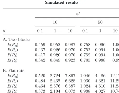
Simulated results
for some i⫽ i1 ⬍ i2 ⬍. . . ⬍ ik⫽ j. In particular, the
global boundB1mis of interest. LetRMdenote the global na bound for haplotypes obtained with Hudson and Kaplan’s
10 50
bij, as defined above.
In the context of unphased data, the boundsbijcould ␣ 0.1 1 10 0.1 1 10 be defined in various ways related to Hudson and
A. Two blocks Kaplan’s. Of interest is
E(RM) 0.459 0.952 0.987 0.758 0.996 1.000
E(Rm) 0.437 0.926 0.970 0.753 0.994 1.000
bk
ij⫽ 1, ifbkij⫺1⫽ 1, ori1,i2, . . . ,ik⫺2exists,
E(R3) 0.417 0.920 0.970 0.752 0.994 1.000
such that (sisi1. . .sik⫺2 sj) isk-incompatible E(R
2) 0.342 0.849 0.923 0.705 0.988 0.999
⫽ 0, otherwise. B. Flat rate
E(RM) 0.520 2.724 7.867 1.046 4.486 12.129
Theorems 1 and 2 provide conditions when b1
ij and b2ij
E(Rm) 0.484 2.435 6.628 1.030 4.321 11.252
are optimal. Forkⱖm, the definition reduces tobk
ij⫽1, E(R
3) 0.464 2.376 6.587 1.024 4.310 11.248
if (sisi⫹1. . .sj⫺1sj) is incompatible, andbijk⫽0 otherwise. E(R
2) 0.373 2.104 6.073 0.938 4.027 10.742
Denote the global bound based onbk ijbyRkM.
an, number of individuals; there are 2nhaplotypes.
Lemma5. For kⱖ 2,
RMⱖRkM⫹1ⱖ RkM, types from which genotype data were obtained by ran-domly pairing haplotypes. This approach makes it
possi-where the genotype bounds, Rk
M, are obtained by randomly
ble to calculateRMandRkMon the same data sets. In all
pairing haplotypes to create individuals.
simulations, the scaled mutation rate per gene (or geno-mic region),, is fixed, ⫽10, and the ratio␣ ⫽ / Let [x,y] denote the interval of integersz, such that
is varied. Here is the scaled recombination rate per
xⱕz ⱕy.
gene. Two models for the recombination process were used: (A) a model with one hotspot in the middle of
Theorem 5.DefineIk⫽(Ik1,Ik2, . . . , Ikik), i⫽ 1, . . . ,
the gene,i.e., two blocks of equal size, and (B) a model
m, recursively by
with flat rate; i.e., recombination happens uniformly along the gene. Table 1 gives a summary of the simula-1. I1⫽(I11), with I1
1⫽[1, 1]and i1⫽1, tions.
2. if sk⫹1is compatible with the sites in Ikik,then ik⫹1⫽ikand Always, R
j
Mⱕ RMⱕ 1 under A. As estimators of the number of blocks the statistics underperform. If the
Ik⫹1⫽(I1k⫹1, . . . ,Ikik⫹⫹11) recombination rate is high, blocks are more easily
in-⫽(Ik
1, . . . ,Ikik⫺1,I k
ik傼 [k⫹1,k⫹1]), ferred. The expected number of segregating sites is E(Sn)⫽ 兺i2⫽n⫺111/i(Watterson1975), which is 34.5 for
3. if sk⫹1is incompatible with the sites in Ikik, then ik⫹1⫽ ik⫹ n ⫽10 and 51.8 for n ⫽50. In consequence, E(S
n)/2 1and
is the average number of variable sites in one block;
e.g.,E(S50)/2⫽ 25.9, ifn⫽50. Ik⫹1⫽ (I1k⫹1, . . . ,Ikik⫹⫹11)
The situation is different for the flat rate model. If ⫽(Ik
1, . . . ,Ikik,I
k⫹1
ik⫹1), with I k⫹1
ik⫹1 ⫽[k⫹1,k⫹1]. is high, then a chromosome becomes distributed onto
many different ancestral genomes in the course of evolu-tionary time. The number of recombination events that
ThenIm⫽(Im1, . . . ,Imim)fulfills: The sites in I
m
j,j⫽1,. .
cause the tree topology to change isⵑ1.5 forn⫽ 10
. , im, are compatible and imis the smallest number of disjoint
and 3.1 forn⫽ 50 (HudsonandKaplan1985). For
intervals with this property. In particular, Rm
M⫽ im⫺1.
␣ ⫽ 0.1 (i.e., ⫽ 1), RM andRmM find only about one-third of all topology changes.
Gusfield’s (2002) algorithm to decide whether a
ma-It transpires that the gain by using R2
M instead of trixS of sites is compatible with a tree has a running
R3
M is in general much larger than the gain by using time of the order ofO(nm). This implies the algorithm
R3
Minstead ofRmMand also that there is a significant gain in Theorem 5 can be implemented with a running time
in knowing the haplotypes rather than just the unphased of the order ofO(nm2).
genotypes. The bounds R2
M, R3M, and RmM were compared to RM
Gene data:Data from two genes were chosen. They via simulations. The neutral coalescent with
recombina-were split into five data sets. The first data set is com-tion, constant population size, and infinite-site mutation
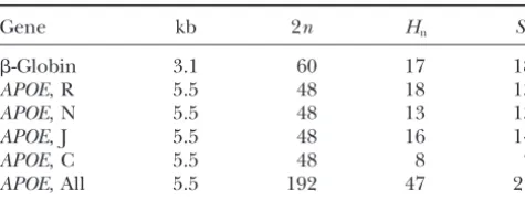
TABLE 3 TABLE 2
The six data sets Summary statistics forRj M
Rm Ma
Gene kb 2n Hn Sn
R3M:a R2
M:a
Gene RM Range Sameb Aveb Aveb Aveb
-Globin 3.1 60 17 18
APOE, R 5.5 48 18 13
-Globin 5 4–5 0.755 4.755 4.755 4.686
APOE, N 5.5 48 13 13
APOE, Rc 6 2–6 0.036 3.427 3.425 3.073
APOE, J 5.5 48 16 14
APOE, Nc 4 2–4 0.572 3.511 3.511 3.146
APOE, C 5.5 48 8 7
APOE, Jc 3 1–3 0.212 1.928 1.927 1.791
APOE, All 5.5 192 47 21
APOE, Cc 1 0–1 0.996 0.996 0.996 0.995
kb, length of gene in kilobases, 2n, number of chromosomes APOE, Allc 9 4–9 0.008 6.158 6.158 5.518
(n is the number of individuals); Hn, number of different
aSummary of 1000 samples generated by randomly pairing haplotypes;Sn, number of SNPs; R, Rochester, Minnesota
(Eu-haplotypes. ropean-American); N, North Karelia, Finland (European); J,
bSame, observed probability that Rj
Mequals RM; Ave, av-Jackson, Mississippi (African-American); C, Campeche,
Mex-erage. ico (Hispanic); and All, R, N, J, and C together.
cSee Table 2.
locus (Fullertonet al.1994). The other four data sets events affect the history of a small fraction of the sample consist of chromosomes sequenced at theAPOEgene only. As a consequence, the LD measure also is affected sampled at four different locations around the world, only marginally. At least naively, this does not seem to each composed of 48 chromosomes (Fullerton et al. be appropriate: Hotspot recombination increases the 2000). In addition, the fourAPOE samples were com- rate of recombination in the region around a hotspot, bined into one data set of 192 chromosomes. Table 2 but should not impose constraints on the time of
partic-provides a summary of the data. ular events.
To investigate the performance ofR2
M,R3M, andRmM, The statistics, RjM,j ⱖ2, discussed in this article do genotypes were generated 1000 times from the haplo- not discriminate between recent and old or sporadic types by randomly pairing haplotypes. The statistics and hotspot events. Some of the break points detected
R2
M, R3M, andRMm were calculated for each of the 1000 by RjM might be due to gene conversion, and others data sets and compared toRM, calculated on the true might be due to recent events affecting only a minority haplotypes. Table 3 shows summaries of the results. For of the haplotypes. Still others might be due to recurrent all data setsR3
MandRmM gave very similar results. How- mutation. Table 4 and the accompanying text showed ever,RMdiffers in some cases sharply fromRmM,e.g., for that when only common haplotypes are taken into
ac-APOE, European-American, andAPOE, All, whereas in count, the results leave the impression of a block-struc-other casesRm
M is in close agreement with RM,e.g., for tured genome. Thus, there is an obvious danger in
over--globin,APOE, European, andAPOE, Hispanic. Overall interpretation of results in favor of block structure. phase information is very useful. It is surprising that the Empirical results are somewhat ambivalent on this African-American sample showed less recombination point. For example, inGabrielet al.(2002) the same than the European-American and European samples. block structures did not show up in all populations, If RM is calculated on only the common haplotypes contrary to what one might expect if blocks are really different results are obtained (see Table 4). Less recom- hotspot delimited. However, due to different demo-bination break points are detected and some sort of
block structure emerges. The same was observed in
sim-TABLE 4
ulated data with a flat recombination rate (results not
shown). It seems that a supposed block structure can Common haplotypes only be an artifact of how the data are analyzed. This is taken
up further in thediscussion. Gene H
n Sn RM
-Globin 5 13 1
DISCUSSION APOE, Ra 4 7 0
APOE, Na 5 7 0
In Gabriel et al.(2002) blocks are defined on the APOE, Ja 4 4 0
basis of a linkage disequilibrium (LD) measure. Roughly APOE, Ca 7 6 1 speaking, two sites are in the same block if LD between APOE, Alla 8 4 3 them is high. A similar procedure is applied inDalyet
Only haplotypes that appear in frequency 5% or higher
al.(2001). Basically, such a procedure tends to cluster are shown.H
n, number of distinct haplotypes;Sn, number of
sites with histories that differ by recent recombination variable sites among common haplotypes. aSee Table 2.
haplotype level: implications for the origin and maintenance of graphic and genealogical histories of populations,
evi-major human polymorphism. Am. J. Hum. Genet.67:881–900. dence for hotspots might fail to show in some popula- Gabriel, S. B., S. F. Schaffner, H. Nguyen, J. M. Moore, J. Royet al., tions and sporadic recombination events might falsely 2002 The structure of haplotype blocks in the human genome.
Science296:2225–2229. be taken as evidence for (nonexisting) hotspots. In
con-Gusfield, D., 1991 Efficient algorithms for inferring evolutionary clusion, there seem to be obstacles to overcome and trees. Networks21:19–28.
more careful analyses to be done before the block-struc- Gusfield, D., 2002 Haplotyping as perfect phylogeny: conceptual framework and efficient solutions, pp. 165–175 inProceedings of tured genome can be claimed as a solid fact.
RECOMB 2002, edited byG. Myers, S. Hannenhalli, D. San-The statisticsRj
M, jⱖ 2, underestimate the number koff, S. Istrail, P. Peuzneret al.ACM Press, New York. of break points compared toRMcalculated on haplotype Hudson, R. R., 1983 Properties of the neutral allele model with
intergenic recombination. Theor. Popul. Biol.23:183–201. data. Another drawback of the statistics Rj
M, j ⱖ 2, is
Hudson, R. R., andN. Kaplan, 1985 Statistical properties of the that they are not able to take frequencies of haplotypes number of recombination events in the history of a sample of into account nor are they able to take the number of DNA sequences. Genetics111:147–165.
Jeffreys, A. J., L. KauppiandR. Neumann, 2001 Intensely punctate different haplotypes into account. (LD measures liker2
meiotic recombination in the class II region of the major histo-andD⬘take SNP frequencies into account.) One of the
compatibility complex. Nat. Genet.29:217–222.
haplotype measures proposed byMyersandGriffiths Johnson, G. C. L., L. Esposito, B. J. Baratt, A. N. Smith, J. Heward et al., 2001 Haplotype tagging for the identification of common (2003) makes use of the number of haplotypes.
How-disease genes. Nat. Genet.29:233–237. ever, it is computationally difficult to generalize their
Myers, S., andR. C. Griffiths, 2003 Bounds on the number of statistic to the case of unphased data. The statistic is recombination events in a sample history. Genetics163:375–394. Watterson, G. A., 1975 On the number of segregating sites in denoted HM and it is always true thatHM ⱖRM.
Essen-genetic models without recombination. Theor. Popul. Biol.7: tially, it compares the number of haplotypes defined by
256–276.
a subset,S, of sites to the number of sites inS. IfHMis Wiuf, C., 2002 On the minimum number of topologies explaining
a sample of DNA sequences. Theor. Popul. Biol.62:357–363. applied to the gene data in this section, it is found that
HM⫽ 7, 11, 5, 6, 2, and 32, for the data sets-globin, Communicating editor: S.Tavare´
APOE, R, N, J, C, and All, respectively. These values should be compared to those obtained by RM: 5, 6, 4, 3, 1, and 9, respectively. Thus, there is a clear benefit
in taking extra information into account. Regions where APPENDIX
HMis high are indicative of hotspots, or multiple
recom-Proof of Theorem1. The “if” part is trivial. The “only if” bination events, whereas regions with lowHM(but⬎0)
goes like this. Consider two sitesi andj. There can at are indicative of gene conversion and sporadic events.
most be two 2’s in a row. Thus, all double heterozygotes Unfortunately, an efficient algorithm for calculation of
insiandsjare in rows with no other 2’s and the
resolu-HM does not exist; therefore there also cannot be an
tion of these does not affect the resolution of other efficient algorithm for calculation of an “unphased”HM.
sites. Further, a compatible resolution of (s1 s2) exists However, approximations ofHMhave proven useful, for
because S is 2-compatible. In conclusion, all pairs of example, using a sliding-window approach or restricting
sites are haplotype compatible andSis compatible. 䊏 the number of sites that are considered at the same time
(see Myers and Griffiths 2003 for details). Similar
Proof of Theorem 2. The last part is trivial because ⵑr techniques might be useful in defining an unphased
resolves sites uniquely. Also, the “only if” is trivial. Now,
HM. An unphased version ofHMmight also be useful in
suppose Shas no 3-incompatibilities. The proof is by addressing questions regarding sporadic events.
induction. Ifk⫽1, 2, or 3 the theorem is trivially true; This article is for, my wife. L. Subrahmanyan is thanked for many
i.e.,Sis compatible and there is a unique compatible useful discussions and suggestions relating to the topic of this article,
resolution. For the induction step assume that the prop-for advice in matters regarding empirical data, and prop-for useful
computa-tional shortcuts. S. R. Kimura is thanked for computacomputa-tional advice. osition is true for k⬘ ⬍ k. The induction basis assures that the first k ⫺ 1 columns are compatible and the resolution is unique. Consider any 2 in thekth column.
LITERATURE CITED If this is the only 2 in that row it cannot create an
incompat-ibility and the phase can be assigned arbitrarily. If more Clark, A., 1990 Inference of haplotypes from PCR-amplified
sam-ples of diploid populations. Mol. Biol. Evol.7:111–122. than one 2 are in the row, choose a sitejand resolvek
Daly, M. J., J. D. Rioux, S. F. Schaffner, T. J. HudsonandE. S.
usingj. This can be done in only one way becausejⵑr k. Lander, 2001 High-resolution haplotype structure in the
hu-If another 2 is in the same row, say, in columni, then it man genome. Nat. Genet.29:229–232.
Estabrook, G., C. JohnsonandF. McMorris, 1975 An idealized cannot create an incompatibility without creating a concept of the true cladistic character. Math. Biosci.23:263–272.
3-incompatibility, becauseiⵑr jandjⵑr k. Thus, allksites Fullerton, S. M., R. M. Harding, A. J. BoyceandJ. B. Clegg, 1994
are compatible. 䊏
Molecular and population genetic analysis of allelic sequence diversity at human-globin locus. Proc. Natl. Acad. Sci. USA91: 1805–1809.
Proof of Lemma1. Reflexivity, symmetry, and transitivity Fullerton, S. M., A. G. Clark, K. M. Weiss, D. A. Nickerson, S. L.
Proof of Lemma 2. The proof is by induction on the cases it follows thatik1ⵑ
r
ik1⫺1cannot be true. In
conse-quence,A⬍⫽ ⭋and the theorem is proved. 䊏
length (kⱖ0) of the sequence introduced below Defi-nition 6: If iⵑe j, then i1, i2, . . . , ik exist, such that
Proof of Corollary1. AssumeF1⬍F2andF2⬍F1. Then
iⵑw i1,i1 ⵑw i2, . . . . , ik⫺1ⵑ w
ik,ikⵑ
w
j. Ifk⫽ 0, then the
result is trivially true. Assume now that it is true for i 僆 F1 andj 僆 F2 exist, such that het(i,j)⫽ 1, i ⬍ j, andj ⬍i. According to Figure 3 one must have i⬇ j.
k⬘ ⬍kand considerk⬘ ⫽k. Thus,i1,i2, . . . ,ikexist, such thatiⵑw i1, . . . ,ikⵑ
w
j. If het(x, y)⫽ 1 for some x, y僆 Leti⬘僆F1be such that,iⵑe i⬘,i⬘⬆ i. Then alsojⵑe i⬘, which contradicts thatF1andF2are disjoint. In conclu-{i,j,i1, . . . ,ik}, {x,y}⬆{i,j}, that are not already joined
byⵑr in the list above, then a smaller sequence can be sion,F1 ⫽{i},F2⫽{j}, andi⬇j. 䊏 extracted with the same property, iⵑw i1,i1ⵑw i2, . . . ,
ik1ⵑ
w
x,xⵑw y,yⵑw ik2, . . . ,ikⵑ
w
j, and in consequence Proof of Corollary 2. The corollary follows from
Theo-rem 3. 䊏
iⵑw j. This follows by application of the induction hy-pothesis twice. If het(x,y)⫽0 for allxandy, then the
Proof of Lemma 3. Only the first part needs a proof. sites in the sequence take the form
The second part is proved in the remark above the lemma. Sincei僆E0only if het(i,j)⫽0 for allj⬆i,j僆
{1, . . . ,m}, then there can at most be one 2 in each row ofS. The result now follows from Theorem 1. 䊏
i i1 i2 … ik–1 ik j
2 2 … z z z
z 2 2 … z z z z z 2 … 2 z z z z z … 2 2 z z z z … z 2 2
2 z z … z z 2
Proof of Lemma4. The first part (E␣⊥E) follows easily
from Lemma 3. To prove the second part (E␣ ⬍ E)
note that all rows with 2’s in E␣ form a subset of the
rows with 2’s for at least onei僆E(Theorem 3). The
phase ofsican be arranged such that all heterozygotes Here, the same row might appear several times, andzis are (0, 1). Thus, ifE
␣ is compatible with E, then the
either 0 or 1 (not necessarily the same value in all places). phase of
E␣can be arranged such that all heterozygotes
Consider the first and the sixth row. It follows thatiⵑr j, in
i僆Eare resolved (0, 1) or are resolved (1, 0). This
and thusiⵑw j, trivially. The lemma is proved. 䊏
proves the lemma. 䊏
Proof of Theorem 3. If het(i, j)⫽ 0 for all i僆 F1 and Proof of Theorem4. Assume that all terminals are
com-j僆F2, theni⊥j. In consequence, the set of rows with patible with a tree. Then the resolution of terminals is heterozygotes inF1 and the set of rows with heterozy- uniquely given. According to Lemma 4, ifE
␣is
compati-gotes inF2are disjoint; otherwise there would beiand
ble withE and E␣ ⬍ E, then E␣ can be resolved in jsuch that het(i,j)⫽ 1.
either of two ways for a given resolution of E. Since
If not het(i,j)⫽0 for alli僆F1andj僆F2, choosei僆
there areM⫺Tnonterminals, it follows there are 2M⫺T
F1, such that het(i,j)⫽1 andi⬍jfor somej僆F2(cf.
compatible resolutions. 䊏
Figure 3). (The casej⬍ iis treated similarly.) Allj⬘僆
F2 belong to one of three sets:A⬍ ⫽ {j⬘|j⬘ ⬍ i}, A⬎ ⫽ Proof of Lemma 5. Note that bk⫹1
ij ⱖbkij, thus also {j⬘|j⬘ ⬎i}, orA⊥⫽{j⬘|j⬘⊥i} (jis inA⬎). Ifi⬍ j⬘and Bk⫹1
ij ⱖ Bkijfrom Equation 2, and the second inequality
j⬘ ⬍ i for somej⬘, then define j⬘to be in A⬎ only. It is proved. To prove the first inequality note that R
M will be proven that A⬍ is empty. Assume, oppositely, remains unchanged ifb
ijis defined by that A⬍ is nonempty and let j⬘ 僆 A⬍. Then j1,
j2, . . . , jk 僆 F2 exist, such that jⵑ
r
i1,j1ⵑr j2, . . . , bij⫽ 1, if sitesiⱕ i⬘ ⬍ j⬘ ⱕjexist,
jk⫺1 ⵑ r
jk,jkⵑ
r
j⬘. Letjk1be the first element amongj1, . . . ,
such thati⬘andj⬘are incompatible
jk, which is not in A⬎ 傼 A⊥. It follows thatjk1⬍i, and
eitheri⬍ jk1⫺1 or i⊥jk1⫺1. According to Figure 3 this ⫽ 0, otherwise.
implies that the genotype pattern schematically takes
It follows from the algorithm given in Hudson and one of the following two forms:
Kaplan(1985). However,bijas defined above fulfillsbijⱖ
i⬍ jk1⫺1 i⊥jk1⫺1 bmij, thusRMⱖRmMⱖRkM, and the inequality is proved.䊏
Proof of Theorem5. Clearly,im⫺1ⱖRmM. To prove the
jk1 i jk1⫺1 jk1 i jk1⫺1
2 2 2 2 2 0
0 2 2 0 2 0
0 0 z 0 z⬘ z
converse let Ijm ⫽ [ij, ij⫹1 ⫺ 1], i1 ⫽ 1, im⫹1 ⫽ m ⫹ 1.
Irrespective of how phase is assigned to the sites inIj⫺1傼
{ij}, 2ⱕjⱕm, eitherijis haplotype incompatible with a site inIj⫺1or two sites inIj⫺1are haplotype incompatible.
Where all 0’s in a column can be replaced by 1’s, rows