Fine Mapping of Complex Trait Genes Combining Pedigree and Linkage Disequilibrium Information: A Bayesian Unified Framework



Fine Mapping of Complex Trait Genes Combining Pedigree and Linkage

Disequilibrium Information: A Bayesian Unified Framework

Miguel Pe´rez-Enciso

1

Institut National de la Recherche Agronomique, Station d’Ame´lioration Ge´ne´tique des Animaux, 31326 Castanet-Tolosan, France Manuscript received September 4, 2002

Accepted for publication December 19, 2002

ABSTRACT

We present a Bayesian method that combines linkage and linkage disequilibrium (LDL) information for quantitative trait locus (QTL) mapping. This method uses jointly all marker information (haplotypes) and all available pedigree information;i.e., it is not restricted to any specific experimental design and it is not required that phases are known. Infinitesimal genetic effects or environmental noise (“fixed”) effects can equally be fitted. A diallelic QTL is assumed and both additive and dominant effects can be estimated. We have implemented a combined Gibbs/Metropolis-Hastings sampling to obtain the marginal posterior distributions of the parameters of interest. We have also implemented a Bayesian variant of usual disequilib-rium measures likeD⬘andr2_{between QTL and markers. We illustrate the method with simulated data}

in “simple” (two-generation full-sib families) and “complex” (four-generation) pedigrees. We compared the estimates with and without using linkage disequilibrium information. In general, using LDL resulted in estimates of QTL position that were much better than linkage-only estimates when there was complete disequilibrium between the mutant QTL allele and the marker. This advantage, however, decreased when the association was only partial. In all cases, additive and dominant effects were estimated accurately either with or without disequilibrium information.

A

N ultimate goal of quantitative trait loci (QTL) stud- ligerand Weiss 1998). In fact, a pure LD analysis is likely to result in a large number of false positives as ies is to clone the gene(s) responsible for the

ge-illustrated recently, e.g., in Alzheimer’s disease ( Ema-netic differences between individuals and, eventually,

hazionet al.2001). identify the causal mutation(s). Certainly, this is a

daunt-A promising approach is thus to combine both link-ing task that will be accomplished only gradually. One

age and linkage disequilibrium (LDL) methods to add of the most severe limitations, at the moment, is that

their advantages in a single unified theoretical frame-the QTL position is estimated with too large an error

work. More specifically, there is an urgent need for to allow positional cloning when a classical linkage

anal-robust methods that provide accurate estimation of the ysis is employed. The 95% confidence interval for the

QTL position. Consider for the sake of illustration a QTL position usually spans over 5–20 cM, at a minimum.

simple design where a number of nuclear families are The wide confidence interval occurs because the

num-typed,i.e., parents and offspring. The theoretical advan-ber of meioses in the genotyped pedigree is usually

tages of combining linkage disequilibrium and pedigree very small; only between two and three generations are

(linkage) information in QTL analysis are manifold: (i) generally employed. Linkage disequilibrium (LD)-based

A marker for which a parent is homozygous does not methods, in contrast, capitalize on the number of

gener-contribute information in a linkage analysis, yet it does ations that occurred since the appearance of mutation

in LD analysis; (ii) conversely, two parents may share and can produce extremely accurate estimates of the

the same haplotype but not necessarily the same QTL gene position, within kilobases in some instances (

Hast-genotypes, and a pure LD analysis would be misleading backaet al.1994). Nevertheless, the chance of success

but the phenotype of offspring together with the ascer-of the LD strategy depends on a number ascer-of population

tainment of alleles transmitted can be used to determine parameters, such as the degree of admixture in the

which are the most likely QTL genotypes of the parents; sampled population, the actual level of association

be-(iii) an individual without relatives but with phenotype tween the causal mutation and the polymorphisms, or

records can be included in the LD analysis, in contrast the correct ascertainment of phases and of genotypes

to a pure linkage study; and (iv) a comparison of the at the QTL. Of course these parameters are usually

analyses including or not the LD information can assess unknown but do dramatically affect the results (

Terwil-the validity of Terwil-the LD model assumptions (i.e., one muta-tion tgenerations ago).

Several authors have addressed the problem of

com-1_{Address for correspondence:INRA, Station d’Ame´lioration Ge´ne´tique}

bining LD and linkage mapping for quantitative trait

des Animaux, BP 27, Cedex 31326 Castanet-Tolosan, France.

E-mail: [email protected] loci (Zhao et al. 1998;Allison et al. 1999;Almasy et

al.1999;Fulkeret al.1999;WuandZeng2001;Farnir (2001), intended for natural populations, is also difficult to apply to complex pedigrees.

et al.2002;Meuwissenet al.2002), whereasXiongand

Here we present a Bayesian method that combines Jin(2000) proposed a method suited to disease

suscepti-linkage and LD information for QTL mapping within bility genes. Zhao et al.(1998) developed a

semipara-a unified theoreticsemipara-al frsemipara-amework. Our LDL method uses metric procedure based on the score-estimating

equa-jointly all marker information, as well as all available tion approach and that addressed the particular case of

pedigree information; i.e., it is not restricted to any single-nucleotide polymorphisms. This is one of the first

specific experimental design and it is not required that articles to provide a theoretical framework for LDL

map-phases be known. If desired, infinitesimal genetic effects ping but the estimating equation approaches are

diffi-or environmental noise (fixed) effects can also be fitted. cult to implement in practice; they require complex

A diallelic QTL is assumed and both additive and domi-computations adapted to each family structure. For

in-nant effects can be estimated. We have implemented a stance, the method sums over all possible phases and

combined Gibbs/Metropolis-Hastings sampling to ob-computes their probabilities, which is extremely

com-tain the marginal posterior distributions of the parame-plex to do in practice beyond a few markers. The

statisti-ters of interest. We illustrate the method with simulated cal properties of these estimators are also unknown.

data. Fulkeret al.(1999) developed a sib-pair analysis in

a likelihood framework. The approach followed by Alli-sonet al.(1999) is a generalization of the transmission

THEORY disequilibrium test (TDT) for quantitative traits (

Alli-son1997), where a between- and within-family associa- We assume that the goal of the analysis is to fine map tion parameter is modeled via a mixed model. Neither a QTL that has been previously located within a given theFulkeret al.(1999) norAllisonet al.(1999) meth- genome region. The genetic model presupposes that a ods are very suited to analyzing complex pedigrees as single mutation occurredt generations ago on a gene affecting the trait studied. Thus, initially, a single ances-they consider sib pairs (Fulkeret al.1999) or

parent-tral (founder) haplotype harbored the mutation. The offspring trios (Allisonet al.1999) and their theoretical

number of haplotypes carrying the mutation increases framework is difficult to generalize to more complex

in successive generations provided that the mutation is settings. TDT in particular is not an optimum choice to

not lost and, due to recombination, the initial allele deal with very polymorphic markers like microsatellites

combination is eroded. The amount of disequilibrium and makes use of only a limited amount of the total

between markers and QTL decreases proportionally to information contained in a typical pedigree.

Meuwis-genetic distance and to the number of generations senet al.(2002), in turn, proposed to model the QTL

elapsed since mutation. Here we use the population alleles as a random variable, where the covariance

be-model for linkage disequilibrium decay described in tween base population haplotypes allows the inclusion

Morris et al.(2000), with modifications described be-of the LD information (Meuwissen and Goddard

low. Briefly, a binary variableSkiis defined such that, at

2000), and the covariance between non-base population

any kth marker locus andith individual, the locus will haplotypes was computed as inFernandoand

Gross-be either identical by descent (IBD) with the original man(1989) andGoddard(1992). They estimated the

haplotype carrying the mutation (Ski⫽ ⫺) or not (Ski⫽

position via maximum likelihood. The model followed

⫹), with minus and plus signs standing for the mutant by these authors is different from the usual LD, where

and wild haplotype alleles, respectively. By convention a diallelic QTL is assumed. The key issue in their method

we denote the QTL by locus 0. A Markov chain Monte is to compute the identity-by-descent probabilities

be-Carlo (MCMC) method was provided by Morriset al. tween the base population haplotypes, and this was done

(2000) to obtain the transition probabilities of a locus by considering the number of identity-by-state alleles

being IBD or not at locusk⫹ 1 conditional on being shared by any two haplotypes, along the lines also

sug-IBD or not at locusk. gested byMcPeek andStrahs (1999). They assumed

Now suppose that the QTL additive and dominance that phases are known, which is a reasonable assumption

effects areaandd, respectively;i.e., the mean phenotype only if families are very large, e.g., as in dairy cattle.

of the individuals homozygous for the wild allele (⫹/⫹) Otherwise, QTL positioning can be dramatically

af-minus that of individuals homozygous for the mutant fected if a phase is incorrectly specified. Farnir et al.

allele (⫺/⫺) is 2a, whereas the mean phenotype of (2002) developed an analytical approach for combining

heterozygous individuals, (⫹/⫺) or (⫺/⫹), is d. Sup-linkage and LD in half-sib families, where the

disequilib-pose further that a numbermof individuals have been rium information is incorporated via Terwilliger’s

typed for DNA markers, contained in matrix M, and (1995) approach. Their method would be very

cumber-that phenotypic measurements (y) are available on a some to generalize to more complex populations; in

subset ofnindividuals. The linear explicative model is addition, phases are assumed to be known and it is not

TABLE 1

Main symbols used

n Number of phenotypic records m Number of individuals in the pedigree

y Phenotypic records, dimensionn

M Marker information, contains the alleles for each individual and marker; dimensionm⫻no. of markers⫻2

S0 Identity-by-descent status of the QTL allele of the base generation individuals with the causative mutation; it can take valueswild(⫹) ormutant(⫺) allele, dimension 2⫻no. of base generation individuals

a Additive QTL effect; the average value of individuals with genotype (⫹/⫹)⫺(⫺/⫺) is 2a d Dominance effect; phenotypic value of individuals with genotype (⫹/⫺) or (⫺/⫹)

u Infinitesimal genetic value; it contains all genetic effects except the QTL under study, dimensionm

␤ Fixed (noise environmental) effects, dimension the sum of levels for each fixed effect

␴2

u Infinitesimal genetic variance ␴2

e Residual variance

␦ QTL position, in morgans

t Time (no. of generations) since mutation

T 2⫻ m matrix with QTL segregation indicators. The genotype of all individuals is unambiguously determined byT

andS0

H Marker phases; contains indicator variable to identify whether the allele in vectorMis of paternal or maternal origin; dimensionm⫻no. of markers

where ␤ is a fixed-effects (environmental/nongenetic p(␪|y,M)⬀p(y,M|␪)p(␪)⫽p(y|␪)p(M|␪)p(␪), (2) effects) vector; wa is a vector with indicator variables

wherep(y,M|␪) is the likelihood (in the Bayesian sense), taking values 1 or ⫺1 if the QTL genotype of each

andp(␪) is thea prioridistribution for the parameters. individual is⫹/⫹ or ⫺/⫺, respectively, and zero for

Note that phenotypes and markers are conditionally heterozygous individuals;wdcontains values 1 if

individ-independent. Ideally, inferences about each of the pa-ual QTL genotype is ⫹/⫺ or ⫺/⫹, zero otherwise;

rameters in␪, say␪l, should be based on the marginal

and u and e contain the infinitesimal genetic values

posterior distribution,i.e., (polygenic effects) and residuals, respectively, whereas

XandZare incidence matrices. The matrixX*contains _{p(␪l|y,M)⫽}

冮

␪⫺l

p(␪l,␪⫺l|y,M)⳵␪⫺l, (3)

Xplus two additional columns forwaandwd; similarly

vector␤* is␤plus elementsaandd. _where␪⫺

lindicates the vector of parameters except the

The goal of the analysis is to obtain estimates of the set _{lth unknown. Typically this multidimensional integral} of parameters,␪⫽{S0,a,d,u,␤,␴2

u,␴2e,␦,t,T,H}, where _{is unfeasible and we need to resort to stochastic}

proce-S0is a matrix containing the IBD status of the two indi- _{dures like Gibbs or Metropolis-Hastings sampling} vidual QTL alleles with the causal mutation, taking val- _{schemes (SorensenandGianola2002). In the} follow-ues ⫹ or ⫺; ␴2

u is the infinitesimal genetic variance; _{ing, we describe all conditional distributions that we}

␴2

e, the residual variance; and␦is the QTL position. T _{need to sample from. Unless otherwise stated, we make}

is a QTL segregation indicator vector containing, for _{the usual assumptions of flat priors for all parameters,} each individual and haplotype, a binary variable speci- _{except forp(u)⫽ Normal(0,A␴}2

u), where Ais the

addi-fying whether the QTL allele is IBD with the paternal _{tive relationship matrix between individuals (Lynchand} or maternal parental allele (Thompson1994). Note that _Walsh1998).

S0 needs to be specified only for the base population The rest of this section is devoted to presenting the

individuals (those without known parents) and that the _{main conditional distributions to sample from to obtain} QTL genotypes for the whole population are unambigu- _{the posterior distribution of the parameters of interest.} ously determined onceS0andT are specified. Finally, For the reader less interested in the mathematical

information, the QTL IBD status of theith base popula-tion individual can be sampled from the fully condi-tional distribution,

p(S0i1,S0i2|y,M,␪⫺) ⬀p(y|␪)p(Mi|␪)p(␪)

⫽

_冤

_兿

j僆⌿i

p(yj|S0i1,S0i2,S0⫺,a,d,ui,␤,␴2e,T)

冥

⫻p(Mi|S0i1,S0i2,t,Hi,␦)⫻p(S0i1,S0i2)

Figure1.—Representation of a pedigree via the

transmis-⫽p(yj僆⌿i|␪)⫻p(Mi|␪)⫻p(S0i1,S0i2),

sion coefficientsT. Each small circle represents an allele of the QTL, identical-by-descent alleles are connected with a

(4)

where yjis the phenotype of the jth individual having

solid line, and individual genotypes, 1–8, are boxed with

received at least one allele from individual i, andS0⫺ dashed lines.

denotes the rest of IBD status not sampled. We now show which are the distributions involved in (4). The first term is a product of Normal densitiesN(ej,␴2e), with

population parameters, like the age of the mutation.

ej ⫽yj⫺xⴕj␤ ⫺uj⫺waja⫺ wdjd,

We assume a star-shaped genealogy. We suppose that

base population individuals are genotyped for most of where, x⬘j is the column vector of X corresponding to the markers but not that phases are known; they are thejth individual’s observation.

inferred from the offspring genotypes. LD or allele fre- The distribution p(Mi|␪) in (4) is the probability of

quency priors do not contribute any information to _{having marker alleles linked in haplotype 1 or 2 (say} obtain the genotypes of the descendant individuals _{Mi1 or Mi2) conditional on a given QTL genotype, its} (conditionally on the genotypes of the base population) _{position relative to DNA markers, and the parameter} and are sampled following the most likely recombinants _{governing the LD decay (t). Both haplotypes are} condi-as inferred from marker information. Once the QTL _{tionally independent; thusp(Mi|␪)⫽p(Mi1, Mi2|S0i1,S0i2,} alleles are sampled, most of the remaining parameters _{t, Hi,␦)⫽ p(Mi1|S0i1,t,Hi, ␦)p(Mi2|S0i2,t, Hi, ␦), where} are obtained via a classical Gibbs sampling within the _{Mi1contains the marker alleles received from the father} mixed-model context (Sorensen andGianola 2002). _{andMi2, those of mother’s origin. Consider the marker} In contrast, Metropolis-Hastings is required for the QTL _{alleles of a given individual i at haplotype h (Mih); in} position; here we identify where recombinants have oc- _{our notation Lmarkers are to the left and Rmarkers} curred at two alternative positions and the resulting _{to the right of the current QTL position. Then,} likelihoods using available phenotypic information are

p(Mih|S0ih,t,Hi,␦)

compared (UimariandSillanpa¨a¨2001).

Base population QTL genotypes (S0):In the absence ⫽_{p(Mih,⫺L, . . . ,Mih,⫺2,Mih,⫺1,Mih1,Mih2, . . . ,MihR|S0ih,t,Hi,}␦₎ of LD information, only the phenotypes of the

individu-⫽p(Mih,⫺L, . . . ,Mih,⫺2,Mih,⫺1|S0ih,t,Hi,␦)

als that have received a given base population allele

provide information about the likely value of that allele. _{⫻p(Mih1,Mih2, . . . ,MihR|S0ih,t,Hi,␦) ⫽QihLQihR,} This is illustrated in the simple pedigree of Figure 1;

whereMihkdenotes the allele at markerk(starting from

the solid lines represent the transmitted alleles, stored

the QTL) of haplotype h, ith individual. Note that k in T. Suppose that we are sampling the IBD status of

takes negative values for markers to the left of the QTL. first individual and first allele (S011), conditional on all

Dropping subscriptsiandhand the conditioning ont, other parameters including the S0 of the remaining

H,and on␦ for clarity, we find individuals (denoted by␪_). The phenotypes of

individ-uals 1, 5, 6, and 7 influence the probabilityp(S011|␪_,y, _QR⫽ _{p(M1,M2, . . . ,MR|S0)}

M). In contrast,p(S012|␪_, y,M), corresponding to the

⫽

_兺

S₁

p(M2, . . . ,MR|S1)p(M1|S1)p(S1|S0).

second QTL allele, involves only the phenotype of indi-vidual 1, as this allele was not transmitted. If that

individ-This process is repeated sequentially from the QTL posi-ual does not have phenotype recorded,p(S012|␪_,y,M)

tion toward the extremes of the interval, is strictly proportional to the prior frequencies for each

QTL allele, when LD information is not being used. We

QR⫽

兺

S1

兺

S2

p(M3, . . . ,MR|S2)p(M2|S2)p(S2|S1)p(M1|S1)p(S1|S0)

denote by␺ithe set of individuals that have received at

least one allele for individual i and have phenotypes,

⫽

_兺

S1

兺

S2

. . .

兺

SR

兿

R

k⫽1

p(Mk|Sk)p(Sk|Sk⫺1), (5)

i.e.,␺1⫽{1, 5, 6, 7},␺2⫽{5, 6}, and␺3⫽ ␺4⫽{3, 4, 8}.

Note that the set␺may vary from iteration to iteration

as a newTis sampled. If LD information is being used, whereSkis the IBD state of marker allelekof individual

p(S0|␪_, y, M) also depends on the marker alleles of iwith the original mutant haplotype.

the original haplotype carrying the mutation (Sk⫽ ⫺) or with the number of markers, especially for highly

poly-morphic markers like microsatellites. However, since not (Sk⫽ ⫹). The term p(Mk|Sk) contains the marker

the relevant statistic is the ratioQ(S0⫽ ⫹)/Q(S0⫽ ⫺),

allele probabilities conditional on Sk; p(Mk|Sk ⫽ ⫹) is

qRandqLcan be initialized to a very large number.

simply given by the population allele frequencies. In

Finally,p(S0i1,S0i2) in Equation 4 is thea priori

proba-contrast,p(Mk|Sk⫽ ⫺) will be 1 for the allele that carried

bility of the IBD state of the two QTL alleles with the the mutant haplotype and 0 for the remaining alleles.

original mutant haplotype. When the individual is not The vector p(M|SL ⫽ . . . S⫺1 ⫽ S1 ⫽ SR ⫽ ⫺) is the

inbred,p(S0i1,S0i2)⫽p(S0i1)p(S0i2), where the prior

prob-original haplotype that carried the mutation. Of course

abilities are the same for any base population allele. If this haplotype is unknown but can be inferred as shown

theith individual is known to be inbred from the avail-byMorriset al.(2000). Here we have preferred to

con-able pedigree with inbreeding coefficientfi,p(S0i1,S0i2)⫽

sider bothSkandp(Mk|Sk) as nuisance parameters;i.e., we

(1⫺fi)p(S0i1)p(S0i2) ⫹ fip(S0i2)␩(S0i1|S0i2), with␩ being

are not usually interested directly in them, and thus we

an indicator 1/0 function that makesS0i1take the same

integrate them out in (5). As a result,p(Mk|Sk⫽ ⫺) is no

value as S0i2. The prior probability of an allele being

longer 0’s and 1’s but can take any value between the two

identical by descent with the original mutant haplotype extremes. Theappendixshows howp(Mk|Sk) is updated.

is␣ if the base population individuals have been sam-The transition probabilitiesp(Sk|Sk⫺1) can be obtained

pled at random from the population,i.e.,p(S0i⫽ ⫺)⫽

as detailed inMorriset al.(2000) and depend on the

␣andp(S0i⫽ ⫹)⫽1⫺ ␣for every individual. Otherwise,

effective size and time since mutation. Four transition

e.g., case/control study or selective genotyping, the probabilities need to be specified, which are

probabilities have to be modified accordingly (Morriset

p(Sk⫽ ⫺|Sk⫺1⫽ ⫺)⫽exp(⫺φt␦k,k⫹1)⫹[1⫺exp(⫺φt␦k,k⫹1)]␣, al.2000).

In summary, to sample the IBD states at the QTL

p(Sk⫽ ⫹|Sk⫺1⫽ ⫺)⫽[1⫺exp(⫺φt␦k,k⫹1)](1⫺ ␣),

position we evaluate Equation 4 at all four possible QTL

p(Sk⫽ ⫺|Sk⫺1⫽ ⫹)⫽[1⫺exp(⫺φt␦k,k⫹1)]␣, genotypes, i.e., (⫹/⫹), (⫹/⫺), (⫺/⫹), (⫺/⫺), for each base population individual in turn, and we take a and _{random number according to the genotype}

probabili-ties. Both alleles are thus sampled simultaneously.

Nev-p(Sk⫽ ⫹|Sk⫺1⫽ ⫹)⫽exp(⫺φt␦k,k⫹1)⫹[1⫺exp(⫺φt␦k,k⫹1)](1⫺ ␣)

ertheless, this strategy can be ameliorated by sampling larger blocks of base population IBD states. Suppose (Morriset al.2000), whereφis the ratio of 1 M/1 Mb

IBD states of base population individuals 1 throughc DNA (typically 1/100),␦k,k⫹1is the distance (morgans)

are sampled; then between loci kand k⫹ 1, and ␣ is the probability of

recombining with a haplotype carrying the mutation.

p(S0i1,S0i2, . . . ,S0c2|y,M,␪⫺)⬀

兿

j僆⌿

p(yj|S0,a,d,ui,␤,␴2e,T)

This parameter is in fact highly confounded with t (Kaplan et al.1995) and we did not try to estimate it;

⫻

_兿

c i⫽1

p(Mi|S0i1,S0i2,t,Hi,␦)

rather, we set␣ ⫽0.001. This had a negligible impact on the results.

Expression (5) is extremely difficult to compute. How- ⫻

_兿

c i⫽1

p(S0i1,S0i2), (6a)

ever, we can rearrange as

where j 僆 ␺ means any individual having received at QR⫽

兺

S₁

p(M1|S1)p(S1|S0) . . .

兺

SR⫺1

p(MR⫺1|SR⫺1)p(SR⫺1|SR⫺2) _{least one allele from any of individuals 1 throughc. An}

issue of interest is to determine whichS0elements are to

⫻

_兺

SR

p(MR|SR)p(SR|SR⫺1). _{be sampled together to minimize the risk of reducibility.}

Here we sampled jointly those origins that coincided in the maximum number of individuals. For instance, if Thus, starting from the outermost marker,R, it is

feasi-only four origins were to be sampled together in the ble to computeQRusing the recursive formula

pedigree of Figure 1, two blocks with the IBD status of qk⫽

兺

Sk

p(Mk|Sk)p(Sk|Sk⫺1)qk⫹1 individuals (1, 2) and (3, 4) rather than (1, 3) and (2,

4) would be chosen. Note that a pure linkage approach can be easily implemented sampling from

with initial valuesq⫺L⫽qR⫽1;QR⫽ 兺1k⫽Rqk, and

simi-larly QL⫽ 兺1k⫽⫺Lqk. Note that each coefficient qk is a

p(S0i1,S0i2, . . . ,S0c2|y,M,␪⫺)⬀

兿

j僆⌿p(yk|S0,a,d,ui,␤,␴

2 e,T)

vector with two elements corresponding to statesSk⫽ ⫹

andSk⫽ ⫺. At the end of the computations we obtain

⫻

_兿

c i⫽1

p(S0i1,s0i2) (6b)

the probabilities of individual haplotypes givenS0 ⫽ ⫹

andS0 ⫽ ⫺. There can be numerical problems in

ob-tainingQR orQLfor a large number of markers as the instead of from (6a).

detailed in theappendix. Once all variables are initial- frequencies were 0.3 and 0.7, whereas there were six alleles at equal frequencies for each microsatellite. The ized, the Markov chain Monte Carlo (MCMC) chain

consists of iterating successively via Equations 4 or 6 QTL was located in position 18 cM, its additive effect was a ⫽ 1, there was no dominance (d ⫽ 0), and the and A2–A7a plus updating the phases (H),p(M|S), and

the transmission indicators (T). Obviously, in a linkage- residual variance was␴2

e ⫽1. Phenotypic records were

simulated for generation 2 in the simple population only approach,(6b), the sampling is simplified by not

samplingp(M|S) and time since mutation (t). The pro- and for all individuals in the complex pedigree. All individuals were genotyped. The mutant QTL allele fre-cedure is otherwise identical.

Two-marker disequilibrium measures: LD measure- quency in the population studied was 0.3. Two situations

were considered: The mutant QTL allele was either ments likeD⬘(Hedrick1987;Lewontin1988) rely on

the possibility of ascertaining the linkage phases and the completely associated with SNP allele “2” (frequency⫽ 0.3) in position 18 cM or partially associated with the alleles themselves, which is not possible with quantitative

traits because the QTL genotypes are not known. Never- SNP allele “1” (frequency ⫽ 0.7). In the former case, all haplotypes with the SNP allele 2 in position 18 cM theless, phases and QTL alleles are generated each

itera-carried the mutant QTL allele; in the latter case, initially tion so we can define a Bayesian estimate ofD⬘between

ⵑ42% (0.3/0.7) of haplotypes with SNP allele 1 har-any marker and the QTL, computingD⬘at the current

bored the QTL mutant allele. The original haplotype configuration using the formula D⬘ ⫽ 兺n1

i⫽1兺2j⫽1piqj|D⬘ij,

carrying the mutation was 1111111111211111 with com-where iis the ith allele of the marker, with frequency

plete association and 1111111111111111 in the second pi, the marker has n1 alleles, index j refers to the jth

case. It was assumed that the mutant allele appeared QTL allele, with frequencyqj, andD⬘ij ⫽Dij/DMAXis the

100 generations ago, and the decay in disequilibrium usual measure for diallelic markers. Here we provided

was simulated following the model in Morris et al. the mean of the posterior distribution, obtained asD⬘

(2000). We compared the results using the LDL method averaged over iterations. We also computed the

recom-(Equation 6a) with those when only linkage information mended measure byPritchardandPrzeworski(2001)

was used (Equation 6b). denoted byr2_(or⌬2_{inDevlinandRisch1995), which}

Three replicates of each case were run, resulting in is defined asr2⫽ 兺n₁

i⫽1兺2j⫽1D2ij/piqj. One of the interesting

12 analyses in total. The only fixed effect included in the properties ofr2_{is thatr}2_{times the number of haplotypes}

analyses was the general mean. The maximum change in is distributed as a chi square with n1 ⫺ 1 d.f. (Weir

QTL position was set to 0.5 cM in each direction. We 1996), although this is an approximation and does not

ran 50,000 iterations of the MCMC chain, discarding hold for larger(Hudson1985). Nevertheless that

prop-the first 4000 iterations. Eight origins were sampled erty is not needed here as we are able to derive the full

jointly; thusp(S0i1,S0i2, . . . ,S0c2|y,M,␪⫺) can take 28⫽

posterior distribution ofr2_{between any marker and the}

256 values because the QTL is assumed to be diallelic. QTL and assess the relevant highest density region that

Phases were updated in blocks of six. Each complete covers the point 0 (no disequilibrium). Here we report

iteration took ⵑ3.5 sec on an alpha workstation with that r⫽

√

r2 _{to make it comparable with} D⬘_{. Both} D⬘

processor 21164A. The computing time per iteration is and rwere calculated using only the base population

highly dependent on the number of paths and phases individuals.

updated simultaneously.

SIMULATION _RESULTS

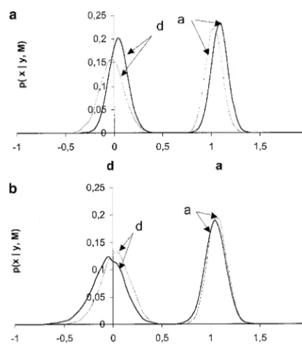
Two population types that can typically be found in _{Table 2 presents the mean and SD of the marginal} livestock, with “simple” and “complex” pedigrees, were _{posterior distributions for the main parameters in the} simulated. The simple population consisted of 40 unre- case of complete association. The posterior distributions lated full-sib families, 10 offspring per family. The com- for the additive and dominant effects in the first repli-plex population was a four-generation pedigree, with a cate are plotted in Figure 2a and provide a whole picture base population of 80 unrelated parents that produced about the uncertainty regarding these parameters. Re-40 full-sib families of size 5 (generation 2), whereas sults were very similar for all replicates so only one is generations 3 and 4 consisted of 20 full-sib families (5 presented. The estimates of the genetic effects and the offspring per family). Parents were chosen at random residual variance were quite accurate, and the SDs of except in generation 1, where all parents had an equal their posterior distributions were small, indicating that number of offspring. Both simple and complex pedi- there is enough information in the data to estimate grees had a total of 480 individuals. The explored region these parameters. The 95% highest density region con-spanned 25 cM and contained six microsatellites at posi- tained the true values of a, d, and ␴2

e in all cases. In

TABLE 2

Posterior distribution statistics: complete association

Parametersc

Pedigreea _{Replicate Analysis}b _a/␴e _d/␴e ␴2

e Position (M) t

Simple 1 LDL 1.06 (0.08) 0.02 (0.10) 0.96 (0.07) 0.169 (0.031) 73 (14) L 1.00 (0.09) ⫺0.05 (0.13) 1.00 (0.07) 0.148 (0.044) — 2 LDL 1.07 (0.08) 0.08 (0.13) 0.99 (0.07) 0.183 (0.027) 79 (20)

L 1.07 (0.10) 0.14 (0.15) 0.99 (0.08) 0.144 (0.062) — 3 LDL 1.08 (0.10) 0.08 (0.10) 0.88 (0.07) 0.180 (0.014) 90 (18)

L 1.02 (0.11) ⫺0.01 (0.12) 0.92 (0.08) 0.192 (0.028) — Complex 1 LDL 0.94 (0.08) ⫺0.05 (0.09) 1.13 (0.08) 0.182 (0.024) 71 (16)

L 0.88 (0.09) 0.01 (0.10) 1.18 (0.09) 0.197 (0.033) — 2 LDL 0.99 (0.08) ⫺0.01 (0.10) 1.03 (0.07) 0.187 (0.020) 101 (21)

L 0.95 (0.09) 0.01 (0.12) 1.07 (0.08) 0.168 (0.042) — 3 LDL 0.96 (0.08) 0.05 (0.09) 1.09 (0.08) 0.169 (0.017) 141 (15)

L 0.91 (0.09) 0.05 (0.10) 1.11 (0.08) 0.160 (0.031) —

All haplotypes with SNP allele 2 carried the QTL mutant allele.

a_{Simple pedigree populations consist of independent full-sib families; complex population is a}

four-genera-tion pedigree with random mating.

b_{LDL analysis combines both linkage disequilibrium and pedigree information; L analysis uses only linkage.} c_{Mean of the marginal posterior distribution (SD of the marginal posterior distribution).}

two competing models. Interestingly, there was little (note that the scales of they-axes are different in Figures 3 and 4). It is also apparent that the mode of the poste-difference between using or not using the linkage

dis-equilibrium information. This means that most, if not rior distribution coincided with the true position only all, information to estimate the QTL genetic effects

comes from classical linkage analysis. The effect of popu-lation structure was also negligible. However, including LD does affect the estimate of the QTL position (Table 2, Figure 3) with complete association between the SNP and the QTL alleles: (1) The mode of the posterior distribution always coincided with the true position and this was not necessarily the case in the linkage-only ap-proach; (2) LDL estimates were always less biased; and (3) the SDs of the posterior distributions were always smaller in the LDL than in the linkage-only method. In general, the relative advantage of LDL over linkage-only was larger in the two-generation than in the complex pedigrees. This can occur because more meioses are available for mapping in the four- than in the two-gener-ation pedigree but also because in the complex pedigree there were fewer offspring per family, making it less accurate for estimating the QTL genotype and the marker phases of the base population individuals, and this has a much larger effect on LDL than in linkage-only analysis.

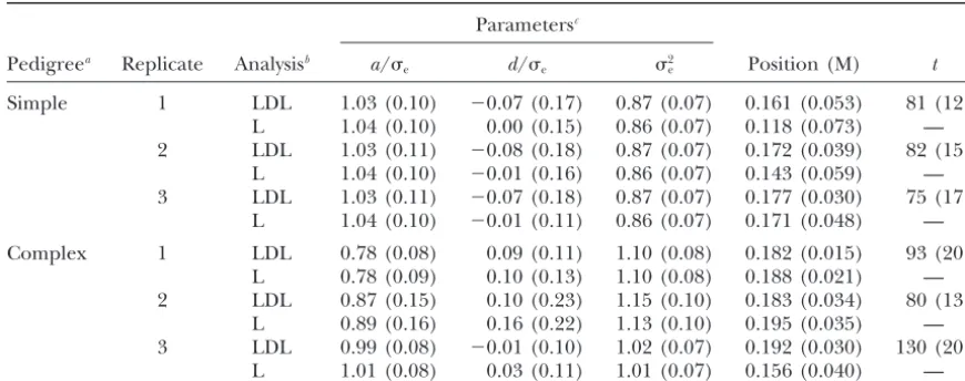
Results concerning the incomplete association sce-nario are presented in Table 3 and Figure 4. As ex-pected, the estimates of the QTL effects were similar to

those in Table 2, albeit the SDs were somewhat larger Figure2.—Marginal posterior probabilities of additive (a) and dominant effects (d), expressed in residual standard devi-in particular for the domdevi-inance effect. Replicate 2 of

ation units. The thick line corresponds to the LDL estimate the complex pedigree had unusually large SD of the

and the thin shaded line, to the linkage-only estimate. (a) posterior distributions ofaandd. But more importantly, _{First replicate of the simple pedigree, complete association;} the accuracy of the QTL position was generally much _{(b) first replicate of the simple pedigree, incomplete}

Figure3.—Marginal posterior proba-bilities of QTL location with complete association between QTL and SNP geno-type. (Left) Simple population graphs; (right) complex population graphs. The three replicates are shown below each other. The solid thick lines refer to esti-mates obtained using linkage and link-age disequilibrium, and the thin shaded lines refer to estimates obtained using linkage information only. The QTL was located in position 18 cM (indicated by the arrowhead).

once (replicate 1, complex pedigree) although it was affect the final results to a large extent, as we found similar output when we fitted these parameters to a close, positions 0.16–0.17 M, in the remaining replicates

with the LDL approach. In some instances (replicate 1, variety of values, in agreement with previous results (MeuwissenandGoddard2000).

simple pedigree) the posterior density was very flat and

covered almost the whole region under study. In princi- Finally, Figure 5 draws a plot of the simple disequilib-rium measures between each marker and the QTL,D⬘ ple, linkage-only estimates should not be greatly affected

by either complete or incomplete association, because andr, for the three simple pedigrees.D⬘andrmeasures obtained under both statistical methods LDL and link-the accuracy depends mainly on link-the informativity of

markers to identify recombinant haplotypes. This seems age-only are plotted. The two top and bottom plots correspond to the complete and incomplete LD scenar-to be the case if we exclude the rather outlying replicate

1 (simple pedigree, Figure 4). The average SD of the QTL ios, respectively. The most striking feature is, perhaps, the extreme differences in behavior betweenD⬘andr. position posterior density was 4 cM in the linkage-only

approach for both complete and incomplete association Under complete LD, the pattern of rwas much more stable behavior than that ofD⬘, as there was very little scenarios. In contrast, it was 2.2 and 3 cM using LDL in

the complete and incomplete scenarios, respectively. variation between replicates andrpeaked clearly at the QTL position (18 cM). In contrast,D⬘had a much larger Contrary to the estimates of QTL genetic effects or

position, the LD decay parametertwas loosely estimated variability between replicates and was clearly multi-modal in several instances. Nevertheless, these two mea-(Tables 2 and 3). This means that there is little

informa-tion in the data to estimate them. In fact, we observed sures showed clear maxima at or close to the true QTL position under complete disequilibrium. The picture that p(M|␪) was quite flat for different values of t. A

TABLE 3

Posterior distribution statistics: incomplete association

Parametersc

Pedigreea _{Replicate Analysis}b _a/␴e _d/␴e ␴2

e Position (M) t

Simple 1 LDL 1.03 (0.10) ⫺0.07 (0.17) 0.87 (0.07) 0.161 (0.053) 81 (12) L 1.04 (0.10) 0.00 (0.15) 0.86 (0.07) 0.118 (0.073) — 2 LDL 1.03 (0.11) ⫺0.08 (0.18) 0.87 (0.07) 0.172 (0.039) 82 (15)

L 1.04 (0.10) ⫺0.01 (0.16) 0.86 (0.07) 0.143 (0.059) — 3 LDL 1.03 (0.11) ⫺0.07 (0.18) 0.87 (0.07) 0.177 (0.030) 75 (17)

L 1.04 (0.10) ⫺0.01 (0.11) 0.86 (0.07) 0.171 (0.048) —

Complex 1 LDL 0.78 (0.08) 0.09 (0.11) 1.10 (0.08) 0.182 (0.015) 93 (20) L 0.78 (0.09) 0.10 (0.13) 1.10 (0.08) 0.188 (0.021) — 2 LDL 0.87 (0.15) 0.10 (0.23) 1.15 (0.10) 0.183 (0.034) 80 (13)

L 0.89 (0.16) 0.16 (0.22) 1.13 (0.10) 0.195 (0.035) — 3 LDL 0.99 (0.08) ⫺0.01 (0.10) 1.02 (0.07) 0.192 (0.030) 130 (20)

L 1.01 (0.08) 0.03 (0.11) 1.01 (0.07) 0.156 (0.040) —

Initially, 43% of haplotypes with SNP allele 1 carried the QTL mutant allele.

a_{Simple pedigree population consists of independent full-sib families; complex population is a}

four-genera-tion pedigree with random mating.

b_{LDL analysis combines both linkage disequilibrium and pedigree information; L analysis uses only linkage.} c_{Mean of the posterior distribution (SD of the posterior distribution).}

Hererhad maxima only at the nearest microsatellites P(M1|S0)⫽

兺

S₁

p(M1|S1)p(S1|S0)

(15 and 20 cM) but a very flat curve was apparent in

clear contrast with the complete LD case. The pattern _and forD⬘was not as affected by incomplete LD (Figure 5,

bottom left) although the profile was somewhat flatter _P(M2|S0)⫽

兺

S₂

兺

S₁

p(M2|S2)p(S2|S1)p(S1|S0)

than that with complete LD. Again, we observed a large

variability between replicates. It is apparent that the LD _⫽

_兺

S₂

p(M2|S2)

兺

S₁

p(S2|S1)p(S1|S0) .

statistics D⬘ and r were higher when using LDL than when using linkage-only methods, although the general

In contrast, we used the actual joint distribution, which pattern was comparable (compare thick solid linesvs.

is thin shaded lines in Figure 5).

P(M1,M2|S0)⫽

兺

S₂

兺

S₁

p(M2|S2)p(S2|S1)p(M1|S1)p(S1|S0)

DISCUSSION

⫽

_兺

S2

p(M2|S2)

兺

S1

p(S2|S1)p(M1|S1)p(S1|S0) .

We have provided a coherent and unified theoretical framework to combine linkage and LD information, as

(Equation 5). Unless complete independence exists exemplified in Equations 4, 6a, and 6b. The method

(which does not make sense in a haplotype analysis), a worked well with simulated data. Here we have used the

joint distribution is not equal to the product of the exponential growth model as described by Morris et

marginals, and our approach should provide more al.(2000) but the Bayesian framework is flexible and

power, even in a LD-only analysis, than that ofMorris other population models can be incorporated by

modi-fyingp(M|␪) appropriately in Equation 4 or 6. An impor- et al.(2000).

tant feature of the method presented here is that it Our results show that it is indeed possible to go be-provides the joint haplotype probability conditional on yond the 20-cM confidence interval to locate QTL in the QTL genotype,i.e.,p(M⫺L, . . .MR, |S0,␪⫺), whereas populations of reasonable size with moderate family

Morris et al. (2000) wrote the likelihood as p(M|S0, sizes and without an extremely dense genotyping. But ␪_) ⫽

兿

kp(Mk|␪), which differs from that used here, they also point out that the advantages of combining

Equation 5. Take, without loss of generality, two mark- LD information into the usual linkage framework ers.Morris et al.(2000, p. 162, bottom) used should not be overemphasized and that its impact may vary dramatically depending on a number of factors. P(M1,M2|S0)⫽ P(M1|S0)P(M2|S0),

Figure4.—Marginal posterior proba-bilities of QTL location with incomplete association between QTL and SNP geno-type. (Left) Simple population graphs; (right) complex population graphs. The three replicates are shown below each other. The solid thick lines refer to esti-mates obtained using linkage and link-age disequilibrium, and the thin shaded lines refer to estimates obtained using linkage information only. The QTL was located in position 18 cM (indicated by the arrowhead).

e.g., on whether there is complete LD between the by the method of computing the posterior distribution from the MCMC samples (Hotiet al.2002). However, marker and the QTL allele. Second, in the population

structure, for accurate LD mapping it is extremely im- the dairy cattle population structure is ideally suited for LD mapping; very large families and small effective portant to determine correctly the phases and the QTL

genotypes. Having a small number of base population population sizes make it possible to accurately estimate phases and QTL genotypes and reduce genetic hetero-individuals with large families seems a better option

than having a complex pedigree spanning several gener- geneity. This is not the case for most livestock species and certainly not the case in humans. Results from the ations, although the optimum structure will depend on

the strength of LD;e.g., if LD is extreme, a large number group of M. Georges are very illustrative (Riquetet al. 1999;Farniret al.2002). Initially,Riquetet al. (1999) of base populations animals will be better because we

will have more “independent” haplotypes. Finally, located a QTL using only LD information, but that posi-tion was shifted to a significantly different posiposi-tion in chance will affect the results: Mendelian transmission,

recombination, and environmental noise are stochastic a later analysis that combined LD and linkage. The primary reason was that sires had different genotypes processes that may result in very different data sets

start-ing from identical initial conditions. A sample of this assigned in each analysis. The population sizes that we used here prevented us from an accurate estimation of variability is in Figures 3 and 4, and very interesting

experimental results are presented,e.g., inEmahazion both the QTL genotypes of base populations and of some of the phases; these two facts together make it et al.(2001).

Our relatively pessimistic conclusions contrast with that no one-to-one correspondence between haplotype and QTL genotype can be established unequivocally. much more optimistic views of the advantages of LDL

mapping in livestock, more specifically in dairy cattle As a result, linkage-only methods do not compare too badly with the LDL strategy. MCMC methods take care (Farniret al.2002;Meuwissenet al. 2002). Of course

parts of the discrepancies are due to the different meth- of the uncertainty but at the price of increasing the variance of the posterior density and thus the accuracy. odological approaches. It should also be mentioned that

equiva-Figure5.—Plots of disequilibrium measures D⬘ and r between each marker and the QTL. The top (bot-tom) row corresponds to the three replicates with complete (incomplete) association in the simple pedigree. Estimates obtained with the LDL method are shown as thick solid lines and those with linkage only, as thin shaded lines. The QTL was located in position 18 cM (indicated by the arrowhead).

tative trait loci mapping. In this case there will be a lents for the classical LD measuresD⬘andr⫽

√

r2_.

In-numbernfof original haplotypes carrying a distinct or

terestingly, r and D⬘ exhibited distinct behaviors

de-the same mutation affecting de-the trait. In our model, this pending on whether there was a complete association

amounts to considering more than either⫹or⫺IBD between the QTL and the SNP (Figure 5);rdecreased

states; an IBD indicator variable should be included and more markedly thanD⬘as we moved away from the QTL

probabilitiesp(M|S0⫽k,k⫽1,nf) should be estimated.

with complete association, but the reverse was true with

In the likely case thatnfis not known, a reversible-jump

incomplete association.NordborgandTavare´(2002)

MCMC strategy could be used. Liu et al. (2001) and have shown that theD⬘measure fluctuates more widely

Morriset al.(2002) have recently presented an alterna-than r, which is in agreement with our results. It is

tive approach to allow for multiple mutations in a pure important to note that there may be a large variability

LD-mapping strategy. Missing markers are dealt with by in disequilibrium decay, as has been evidenced by

simu-using only available information for computing phases lation (e.g.,Nordborg andTavare´ 2002;Pritchard

and segregation indicators. This is a reasonable approxi-andPrzeworski2001) or with experimental data (Reich

mation if the percentage of missing genotypes and the et al.2001). In particular, it is difficult to compare LD

pedigree’s complexity are not large; otherwise the trans-measures of SNPs with those of microsatellites.

Disequi-mission coefficientsTare not properly calculated. This librium measures depend necessarily on allele

frequen-should not be too much of a concern in the special case cies and, as argued (Nordborg and Tavare´ 2002),

of fine mapping, where one is usually analyzing a few they should because gene history and frequency are

generations and very dense genotyping. However, this inextricably linked. Here disequilibrium measures

de-is a much more important limitation in marker-assde-isted creased much more rapidly with SNPs than with

multial-selection or in linkage analysis of complex populations. lelic markers. It is also important to bear in mind that

Here we have implicitly assumed a star-shaped geneal-the pattern in disequilibrium decay between QTL and

ogy, which is not realistic in many instances. The depen-marker does not necessarily parallel the posterior

distri-dence among sampled base population haplotypes,i.e., bution of the QTL position, as is evident from

compar-the fact that recombination histories are correlated, can ing the graphs in Figures 3 and 4 (simple pedigree)

be included in the model via,e.g., coalescent techniques with those in Figure 5.

assuming a given effective size (Meuwissenand God-Certainly, further extensions and testing of this

ap-dard2001). A simple strategy is to consider that prior proach are warranted, particularly to overcome some

allele states in any two haplotypes are not independent, of the potential risks of using LD. First of all,

stratifica-i.e.,p(S0i,S0i⬘)⬆p(S0i)p(S0i⬘), but rather use the additive

tion may cause spurious disequilibrium. In principle, a

relationship coefficient (␳i,i⬘), computed using all

avail-LDL methodology should be more robust than a pure

able pedigrees as a measure of association; thenp(S0i,

LD strategy but this remains to be tested and it is

uncer-S0i⬘)⫽(1 ⫺ ␳ii⬘)p(S0i)p(S0i⬘)⫹ ␳ii⬘ p(S0i)␩(S0i|S0i⬘), as

ex-tain whether stratification has such a large impact on

plained in thetheorysection. Much more complicated quantitative traits mapping as it does with binary traits.

pedi-Janss, L. L. G., R.Thompsonand J. A.Van Arendonk, 1995

Applica-gree previous to the first genotyped individuals and

tion of Gibbs sampling for inference in a mixed major

gene-their observed marker alleles. _{polygenic inheritance model in animal populations. Theor. Appl.} To conclude, fine mapping complex trait genes is a Genet.91:1137–1147.

Kaplan, N., W. G. HillandB. S. Weir, 1995 Likelihood methods

topic of very active research and a major challenge in

for locating disease genes in nonequilibrium populations. Am.

both human and animal genetics. Given the diversity _{J. Hum. Genet.56:18–32.}

of genetic architectures and population histories, it is Lewontin, R. C., 1988 On measures of gametic disequilibrium. Ge-netics120:849–852.

unlikely that a single statistical approach will be valid

Liu, J. S., C. Sabatti, J. Teng, B. J. KeatsandN. Risch, 2001

Bayes-for all cases. One of the advantages of the Bayesian _{ian analysis of haplotypes for linkage disequilibrium mapping.} approach presented here is that the different sources Genome Res.11:1716–1724.

Lynch, M., andB. Walsh, 1998 Genetic Analysis of Quantitative Traits.

of knowledge are conditionally independent (Equations

Sinauer, Sunderland, MA.

4 and 6) so that we can consider,e.g., different popula- _{McPeek, M. S., andA. Strahs, 1999 Assessement of linkage} disequi-tion genetic models to model LD simply by changing librium by the decay of haplotype sharing, with application to fine scale genetic mapping. Am. J. Hum. Genet.65:858–875.

equationp(M|␪) appropriately. Additionally, the degree

Meuwissen, T. H. E., andM. E. Goddard, 2000 Fine mapping of

of uncertainty about the parameters can be fully

de-quantitative trait loci using linkage disequilibria with closely

scribed via the marginal posterior distribution. linked marker loci. Genetics155:421–430.

Meuwissen, T. H., andM. E. Goddard, 2001 Prediction of identity We are thankful for helpful discussions with M. Sillanpa¨a¨, D. Milan, _{by descent probabilities from marker-haplotypes. Genet. Sel. Evol.} J. M. Elsen, B. Goffinet, and L. L. G. Janss. A referee is thanked for _{33:605–634.}

the suggestions. This work was funded by the Bureau des Ressources _{Meuwissen, T. H., A. Karlsen, S. Lien, I. OlsakerandM. E.} God-Ge´ne´tiques, project no. 20, and Action en Bioinformatique (France). dard, 2002 Fine mapping of a quantitative trait locus for twin-ning rate using combined linkage and linkage disequilibrium mapping. Genetics161:373–379.

Morris, A. P., J. C. WhitakerandD. J. Balding, 2000 Bayesian fine-scale mapping of disease loci, by hidden Markov models.

LITERATURE CITED

Am. J. Hum. Genet.67:155–169.

Allison, D. B., 1997 Transmission-disequilibrium tests for quantita- _{Morris, A. P., J. C. WhittakerandD. J. Balding, 2002 Fine-scale} tive traits. Am. J. Hum. Genet.60:676–690. _{mapping of disease loci via shattered coalescent modeling of}

Allison, D. B., M. Heo, N. KaplanandE. R. Martin, 1999 Sibling- _{genealogies. Am. J. Hum. Genet.70:686–707.}

based tests of linkage and association for quantitative traits. Am. _{Nordborg, M., andS. Tavare´, 2002 Linkage disequilibrium: what}

J. Hum. Genet.64:1754–1763. _{history has to tell us. Trends Genet.18:83–90.}

Almasy, L., J. T. Williams, T. D. DyerandJ. Blangero, 1999 Quan- _{Pritchard, J. K., andM. Przeworski, 2001 Linkage disequilibrium} titative trait locus detection using combined linkage, disequilib- _{in humans: models and data. Am. J. Hum. Genet.69:1–14.} rium analysis. Genet. Epidemiol.17(Suppl. 1): S31–S36. _{Reich, D. E., M. Cargill, S. Bolk, J. Ireland, P. C. Sabetiet al.,}

Devlin, B., andN. Risch, 1995 A comparison of linkage disequilib- _{2001 Linkage disequilibrium in the human genome. Nature} rium measures for fine-scale mapping. Genomics29:311–322. _{411:199–204.}

Emahazion, T., L. Feuk, M. Jobs, S. L. Sawyer, D. Fredmanet al., _{Riquet, J., W. Coppieters, N. Cambisano, J. J. Arranz, P. Berziet} 2001 SNP association studies in Alzheimer’s disease highlight

al., 1999 Fine-mapping of quantitative trait loci by identity by problems for complex disease analysis. Trends Genet.17:407– _{descent in outbred populations: application to milk production} 413.

in dairy cattle. Proc. Natl. Acad. Sci. USA96:9252–9257.

Farnir, F., B. Grisart, W. Coppieters, J. Riquet, P. Berziet al., _{Satagopan, J. M., B. S. Yandell, M. A. NewtonandT. C. Osborn,} 2002 Simultaneous mining of linkage and linkage

disequilib-1996 A Bayesian approach to detect quantitative trait loci using rium to fine map quantitative trait loci in outbred half-sib pedi- _{Markov chain Monte Carlo. Genetics}

144:805–816. grees: revisiting the location of a quantitative trait locus with

Sillanpaa, M. J., andE. Arjas, 1998 Bayesian mapping of multiple major effect on milk production on bovine chromosome 14.

quantitative trait loci from incomplete inbred line cross data. Genetics161:275–287.

Genetics148:1373–1388.

Fernando, R. L., andM. Grossman, 1989 Marker assisted selection

Sorensen, D., andD. Gianola, 2002 Likelihood, Bayesian, and McMc

using best linear unbiased prediction. Genet. Sel. Evol.21:467–

Methods in Quantitative Genetics. Springer Verlag, New York. 477.

Terwilliger, J. D., 1995 A powerful likelihood method for the

Fulker, D. W., S. S.Cherny, P. C.Shamand J. K.Hewitt, 1999

analysis of linkage disequilibrium between trait loci and one or Combined linkage and association sib pair analysis for

quantita-more polymorphic marker loci. Am. J. Hum. Genet.56:777–787. tive traits. Am. J. Hum. Genet.64:259–267.

Terwilliger, J. D., andK. M. Weiss, 1998 Linkage disequilibrium

Goddard, M. E., 1992 A mixed model analysis of data on multiple

mapping of complex disease: Fantasy or reality? Curr. Opin. Bio-genetic markers. Theor. Appl. Genet.83:878–886.

technol.9:578–594.

Hastbacka, J., A. de la Chapelle, M. M. Mahtani, G. Clines,

Thompson, E. A., 1994 Monte Carlo likelihood in genetic mapping.

M. P. Reeve-Dalyet al., 1994 The diastrophic dysplasia gene

Stat. Sci.9:355–366. encodes a novel sulfate transporter: positional cloning by

fine-Uimari, P., and I. Hoeschele, 1997 Mapping-linked quantitative structure linkage disequilibrium mapping. Cell78:1073–1087.

trait loci using Bayesian analysis and Markov chain Monte Carlo

Heath, S. C., 1997 Markov Chain Monte Carlo segregation and

algorithms. Genetics146:735–743. linkage analysis for oligogenic models. Am. J. Hum. Genet.61:

Uimari, P., andM. J. Sillanpa¨a¨, 2001 Bayesian oligogenic analysis 748–760.

of quantitative and qualitative traits in general pedigrees. Genet.

Hedrick, P. W., 1987 Gametic disequilibrium measures: proceed

Epidemiol.21:224–242. with caution. Genetics117:331–341.

Wang, C. S., J. J. RutledgeandD. Gianola, 1993 Marginal

infer-Henderson, C. R., 1984 Applications of Linear Models in Animal

Breed-ences about variance components in a mixed linear model using

ing. University of Guelph, Guelph, ON, Canada.

Gibbs sampling. Genet. Sel. Evol.25:41–62.

Hoti, F. J., M. J. SillanpaaandL. Holmstrom, 2002 A note on

Weir, B. S., 1996 Genetic Data Analysis II. Sinauer, Sunderland, MA. estimating the posterior density of a quantitative trait locus from

Wu, R., andZ-B. Zeng, 2001 Joint linkage and linkage disequilibrium a Markov chain Monte Carlo sample. Genet. Epidemiol.22:369–

mapping in natural populations. Genetics157:899–909. 376.

Xiong, M., andL. Jin, 2000 Combined linkage and linkage

disequi-Hudson, R. R., 1985 The sampling distribution of linkage

disequilib-librium mapping for genome screens. Genet. Epidemiol.19:211– rium under an infinite alleles model without selection. Genetics

Zhao, L. P., C. Aragaki, L. HsuandF. Quiaoit, 1998 Mapping of _{at markerkthe alleles are IBD with the mutant} haplo-complex traits by single nucleotide polymorphisms. Am. J. Hum.

type are calculated given the IBD state at the QTL

posi-Genet.63:225–240.

tion,S0equaling either⫹or⫺. The original frequencies Communicating editor: C.Haley

of allelejat markerkin the nonmutant population are obtained from

APPENDIX: SAMPLING DISTRIBUTIONS

p(Mkj|Sk⫽ ⫹,␪_)⫽

兺

F

i⫽1

兺

2

h⫽1

p(Skih⫽ ⫹|S0ih)␩ihjk/(2F) ,

Mixed-model effects (a, d, u, and ␤): The

mixed-model equations (Henderson1984) are, conditional _{whereFis the number of base population haplotypes,} onwa,wd,␴2

u, and␴2e, ␩

ihjkis an indicator variable taking value⫽1 if the

individ-ualihas allelejat markerkand haplotypeh, and zero

冤

X*ⴕX* ZⴕX*

X*ⴕZ ZⴕZ⫹ A⫺1␭

冥 冤

␤*

u

冥

⫽

冤

X*ⴕy

Zy

冥

, (A1) otherwise. Similarly, we compute p(Mkj|Sk⫽ ⫺,␪_)⫽

兺

F

i⫽1

兺

2

h⫽1

p(Skih⫽ ⫺|S0ih)␩ihjk/(2F) ,

orCb⫽d, whereCis the left-hand-side matrix in (A1) above, d is the right-hand-side vector, and b contains

which is the probability that the original mutant

haplo-␤*andu, with␭ ⫽ ␴2

e/␴2u.Wanget al.(1993) showed

type contains allelejat markerk. An alternative option that the fully conditional distribution of any elementbi

is to sample the original mutant haplotype as inMorris ofb⫽[␤*,u] is

et al.(2000). However, and unless we are interested in reconstructing the original haplotype, we prefer the biⵑNormal(di⫺

兺

N

j⫽1,j⬆i

cijdj,␴2e/cii), (A2)

approach here, whereby the founder haplotype, that where QTL mutation occurred, is treated as a nuisance wherediis theith element of the right-hand-side vector,

parameter and integrated out. andcijis element (i,j) ofC, which has dimensionN.

Phase sampling (H):Phases that could not be

deter-Variance components (␴2

uand␴2e): The fully

condi-mined unambiguously were sampled using a block tional distributions are

Gibbs sampling algorithm. A parameterizable number of marker phases were sampled jointly for each individ-p(␴2

u|S0,a,d,u,␤,␴2e,y)⫽ (uⴕA⫺1u)␹⫺m2 (A3)

ual in turn. The algorithm works as follows. First, un-known phases for a given individual are identified, say and

nh unknown phases. Second, an indicator variable is

constructed taking all possible values (2n_{h). For instance,}

p(␴2

e|S0,a,d,u,␤,␴2u,y)⫽(y⫺X*␤*⫺Zu)⬘

suppose that there are four markers and that the phases

⫻(y⫺X*␤*⫺Zu)␹⫺2

n (A4) _{of first and last markers are known or not sampled (i.e.,}

missing marker), then the indicator variable may take (Wang et al. 1993), where ␹⫺2

q stands for an inverted

values ⫺00⫺, ⫺01⫺, ⫺10⫺, and ⫺11⫺, where “⫺” chi-square distribution withqd.f. Equations A3 and A4

stands for not sampled, “0” for paternal, and “1” for assume a naı¨ve ignorance prior. Conjugate informative

maternal origin. Finally, the probability associated with priors with prior varianceO2_and␯_{d.f., respectively,}

re-each value is calculated using all available marker infor-sult in posteriori conditional distributions of the type

mation and current phases in parents and offspring and (QF⫹O2_␯)␹⫺2

q⫹␯, where QF is the quadratic form in (A3)

a new phase block is sampled. Here a maximum of six or (A4) (Wang et al. 1993; Sorensen and Gianola

phases were sampled jointly. 2002).

Segregation indicators (T): Twas usually updated

to-Linkage disequilibrium parameters [t, p(Mk,j|Sk)]:The

gether with the QTL position, as explained below. A fully conditional distribution oftis not a known

distribu-new proposal forTwas sampled conditioning on marker tion and, thus, we resort to Metropolis-Hastings

sam-and phase information using Mendelian rules. pling. A new proposed age of mutationtnew_{is accepted}

with probability QTL position (␦): This is one of the most critical steps of the Bayesian procedure. A variety of strategies have been proposed in the literature (Satagopan et min

冦

1,p(M|S0,t

new_,H,␦₎

p(M|S0,t,H,␦)

冧

. (A5)

al.1996; Heath 1997; Uimari and Hoeschele 1997; Sillanpaa and Arjas 1998). In a typical sampling scheme, individualS0would be updated conditional on

The probabilitiesp(Mkj|Sk) contain the allele

probabili-the oprobabili-ther genotypes, but this is a risky option as probabili-the ties for each allelejof markerkconditional on the IBD

chain will get stuck easily (Jansset al. 1995).Uimariand state of the marker with the original mutant haplotype.

Sillanpa¨a¨(2001) proposed a dual sampling scheme. In This variable is updated each iteration as follows. For

as described using a new position,␦new_{, and both T}new

min

冦

1,p(T|␦

new_,H)

p(T|␦,H)

冧

. (A6) and␦newwere accepted with probability min

冦

1,p(y|T

new_,S

0,a,d,u,␤,␴2e)

p(y|T,S0,a,d,u,␤,␴2e)

冧

(A6⬘) However, using (A6) may prevent ␦ from “jumping”

between adjacent marker intervals because the above

acceptance ratio is very sensitive to the percentage of (UimariandSillanpa¨a¨2001). OtherwiseT and␦ re-QTL recombinant haplotypes, which in turn depends mained unchanged. Here, sampling was normally per-on the marker interval. In other iteratiper-ons T and ␦ formed via (A6⬘), except every five iterations when (A6)