A Haplotype-Based Algorithm for Multilocus Linkage Disequilibrium Mapping of Quantitative Trait Loci With Epistasis



A Haplotype-Based Algorithm for Multilocus Linkage Disequilibrium

Mapping of Quantitative Trait Loci With Epistasis

Xiang-Yang Lou,*

_{George Casella,* Ramon C. Littell,* Mark C. K. Yang,*}

Julie A. Johnson

_{and Rongling Wu*}

*Department of Statistics,‡_{Department of Pharmacy Practice, University of Florida, Gainesville, Florida 32611 and} †_{Department of Agronomy, Zhejiang University, Hangzhou, Zhejiang 310029, People’s Republic of China}

Manuscript received October 7, 2002 Accepted for publication January 16, 2003

ABSTRACT

For tightly linked loci, cosegregation may lead to nonrandom associations between alleles in a population. Because of its evolutionary relationship with linkage, this phenomenon is called linkage disequilibrium. Today, linkage disequilibrium-based mapping has become a major focus of recent genome research into mapping complex traits. In this article, we present a new statistical method for mapping quantitative trait loci (QTL) of additive, dominant, and epistatic effects in equilibrium natural populations. Our method is based on haplotype analysis of multilocus linkage disequilibrium and exhibits two significant advantages over current disequilibrium mapping methods. First, we have derived closed-form solutions for estimating the marker-QTL haplotype frequencies within the maximum-likelihood framework implemented by the EM algorithm. The allele frequencies of putative QTL and their linkage disequilibria with the markers are estimated by solving a system of regular equations. This procedure has significantly improved the computational efficiency and the precision of parameter estimation. Second, our method can detect marker-QTL disequilibria of different orders and QTL epistatic interactions of various kinds on the basis of a multilocus analysis. This can not only enhance the precision of parameter estimation, but also make it possible to perform whole-genome association studies. We carried out extensive simulation studies to examine the robustness and statistical performance of our method. The application of the new method was validated using a case study from humans, in which we successfully detected significant QTL affecting human body heights. Finally, we discuss the implications of our method for genome projects and its extension to a broader circumstance. The computer program for the method proposed in this article is

available at the webpage http://www.ifasstat.ufl.edu/genome/ⵑLD.

D

associa-tion leading to cosegregaassocia-tion of different genes affect mal breeding and evolutionary studies, the genetic

basis of a quantitatively inherited trait has not been gamete distribution and frequencies and, thus, are

con-sidered to be population genetic parameters (Mackay

well understood. Two factors have caused this. First,

a quantitative trait, or a complex trait, is likely to be 2001).

controlled by many genes, each having a small effect Apart from possible allelic associations, different

(LynchandWalsh1998). Such genes are difficult to genes may be mutually dependent when one gene

pre-identify using classic genetic approaches. Second, as vents another from manifesting its effect through a

par-revealed in a considerable body of literature, the genes ticular biochemical pathway (Phillips1998). Such

de-underlying a complex trait are not independent in ex- pendence of genes is referred to asepistasis, a ubiquitous

erting an effect on quantitative variation (reviewed in phenomenon in the genetic control of a complex trait.

Mackay2001). The dependence between alleles at dif- Epistasis, described as a type of gene interaction on

ferent loci may be due to their linkage on the same phenotypes, possesses the property of a quantitative

ge-chromosome or nonrandom association even if they are netic parameter. Classical estimation of quantitative

ge-on different chromosomes. In particular, the nge-onran- netic parameters is based on the resemblance among

dom association between two linked genes is calledlink- relatives using a theory established byFisher (1918),

age (gametic) disequilibrium (Risch and Merikangas but this approach lacks the power to estimate epistasis

1996;Hudson2000). Unlinked genes may also be asso- because epistasis contributes little to the relative

resem-ciated if biological processes, such as population differ- blance. A lack of powerful methods for estimating

epista-entiation, population admixture, and natural selection, sis has diminished its central role in trait evolution and

domestication, as claimed by S. Wright and his followers

(Wolfet al.2000).

The advent of complete DNA-marker linkage maps

1_{Corresponding author:Department of Statistics, 533 McCarty Hall C,}

University of Florida, Gainesville, FL 32611. E-mail: [email protected] has provided a powerful tool for investigating the

netic architecture of a quantitative trait in plants, ani- natural population. Our method has been validated by the successful detection of QTL for human body height.

mals, or humans (reviewed in Mackay2001; Barton

andKeightley2002). A number of statistical methods have been proposed to map genes responsible for

com-POPULATION GENETIC MODEL

plex traits, referred to as quantitative trait loci (QTL),

based on different genetic designs, different marker _{Suppose there is a panmictic natural population, in}

types, and different mapping populations (reviewed in _{whichmbiallelic markers,ᏹ}

1,ᏹ2, . . . ,ᏹm, andqbiallelic Jansen2000;Hoeschele2000). Most of these methods _{QTL, ᏽ}1_,ᏽ2_{, . . .} ᏽq_{, are segregating. For the sake of}

were developed to adapt gene segregation patterns in _{distinction, we use the subscripts to denote the markers}

a mapping pedigree derived from a controlled cross _{and the superscripts to denote the QTL. Two alleles at}

and have two significant limits when they are applied _{a locus are denoted by M}1

k and M2k, or indexed by rk

on a wider scheme. First, for many species such as hu- _(r

k⫽ 1, 2), for markerᏹk, andQl1andQl2, or indexed

mans, it is not possible to obtain controlled crosses and _bys

l(sl⫽1, 2), for QTLᏽl. This population is assumed

thus their QTL mapping should be based on existing _{to be in disequilibrium, so that all markers and QTL}

natural populations. Second, many methods assume _{are associated with one another. We denoteD}

k₁k₂as the

that epistatic effects due to gene interaction are absent, _{coefficient of digenic linkage disequilibrium between}

to facilitate the estimation of quantitative genetic pa- _markersᏹk

1 and ᏹk2, D

l1l2 _{as the coefficient of digenic}

rameters. Given the complexity of quantitative variation, _{linkage disequilibrium between QTL ᏽ}l1 _and ᏽl2 _and

however, the assumption of no epistasis most likely devi- _Dl₁

k₁as the coefficient of digenic linkage disequilibrium

ates from biological reality (Mackay2001;Bartonand _{between markerᏹk}

1and QTLᏽ

l_{1. Similarly, the}

coeffi-Keightley2002). _{cients of trigenic (D}l₁

k1k2andD l₁l₂

k1), quadrigenic (D

l₁l₂ k1k2), or

In this article, we present a new statistical method for _{higher-order linkage disequilibrium can be defined.}

mapping QTL with epistasis in natural populations. Our _{Haplotypes, zygote configurations, and zygote}

geno-analysis is based on an important population property _{types:With the above notation for the markers and QTL}

of gene segregation, that is, linkage disequilibrium _{and their corresponding alleles, a general multilocus}

(LynchandWalsh1998;Hudson2000), although this _{haplotypemix for the markers (M1 M2. . .M}

m) and the

property made quantitative genetic study more difficult _{QTL (Q}1_Q2_{. . .Q}q_{) is denoted byg}s₁s₂...s_q

r₁r₂...r_m(r1, . . . ,rm;s1,

in the past. Linkage causing linkage disequilibrium is _{. . . , s}

q⫽ 1, 2), with population frequency expressed

used as a basis for fine mapping of human diseases _asps₁s₂...s_q

r₁r₂...r_m. This haplotype frequency can be divided into

(Templeton1999) and has been successful in several _{the allele frequencies and a set of disequilibrium}

coeffi-case studies of gene positional cloning (reviewed in _{cients of different orders (Hudson2000). For example,}

Ardlie et al.2002).Luo andSuhai(1999), Luoet al. _{when there is no interference between recombinations,}

(2000), andWuet al.(2002) extended disequilibrium- _{a one-marker (ᏹk)/one-QTL (ᏽ}l_{) haplotype frequency}

based mapping strategies to map QTL for a quantitative _{is divided into two parts, no disequilibrium and digenic}

trait using a random sample drawn from a natural popu- _{disequilibrium, expressed as}

lation. However, in these studies only the simplest

model, based on one marker and one QTL, was formu- No disequilibrium psl

r_k⫽ pr_kpsl

Digenic disequilibrium ⫹(⫺1)r_k⫹s_lDl

k.

(1) lated. The application of these models to study the

ge-netic architecture of polygenic traits is therefore limited.

Our model presented here uses a multilocus linkage _{From now on we omit the symbolskfor markers andl}

disequilibrium analysis to detect epistatic QTL and esti- _{for QTL for simplicity, unless they are needed. A}

two-mate the effects of their gene action and interaction on _{marker/one-QTL haplotype frequency is expressed as}

a quantitative trait. Our model can be considered to be comprehensive, because it includes all possible disequi-libria among different markers and QTL and considers

No disequilibrium ps

r1r2⫽pr1p

s_p r2

3 digenic disequilibria ⫹(⫺1)s⫹r2p_r

1D

l k2⫹(⫺1)

r1⫹sp_r 2D

l k1

⫹(⫺1)r1⫹r2psD_k 1k2

1 trigenic disequilibrium ⫺(⫺1)r1⫹r2⫹sDl_k

1k2.

quantitative gene interaction effects of different kinds.

We derive a simple closed form of the expectation-max- (2)

imization (EM) algorithm for estimating the allelic fre- _{When four or more genetic loci are associated,}

disequi-quencies and coefficients of linkage disequilibria and _{libria of one set of loci may interact with those of other}

gene action and interaction effects. Because of this com- _{sets to form so-called multiplicative disequilibria (}

Ben-putational innovation, the estimation precision of QTL _{nett1954). When (at least two) epistatic QTL are}

asso-population and quantitative parameters from our _{ciated with multiple markers, these multiplicative}

dis-multilocus model can be significantly improved over _{equilibria should be considered. For example, under}

that of traditional treatments, despite the fact that the _{the assumption of no interference between}

recombina-multilocus model contains an increasingly larger num- _{tion events (Bennett 1954), a four-marker/two-QTL}

ber of unknown parameters. Extensive simulations are _{haplotype frequency is expressed as}

performed to study the robustness and performance of

ps1s2

r1r2r3r4⫽

No disequilibrium different alleles at the same locus, the number of zygote configurations may be greater than the number of zy-pr1pr2pr3pr4p

s1ps2

gote genotypes. For example, zygote genotypeG{12}

{11}{12}is

15 digenic disequilibria

generated via configurationg1

11⫻g212org211⫻ g112.

⫹(⫺1)r3⫹r4p_r 1pr2p

s1ps2D_k

3k4⫹. . .⫹(⫺1)

s1⫹s2p_r 1pr2pr3pr4D

l1l2

Of the eight three-locus haplotype frequencies

con-20 trigenic disequilibria

tained in the joint probability matrix of Table 1, seven

⫺(⫺1)r2⫹r3⫹r4p_r 1p

s1ps2D_k

2k3k4⫺. . .⫺(⫺1)

r1⫹s1⫹s2p_r 2pr3pr4D

l1l2

k1

are independent because of the constraint 兺2

r₁⫽1兺r2₂⫽1

15 quadrigenic disequilibria

兺2

s⫽1psr₁r₂⫽1. These seven independent frequencies,

ar-⫹(⫺1)r1⫹r2⫹r3⫹r4ps1ps2D_k

1k2k3k4⫹. . .⫹(⫺1)

r1⫹r2⫹s1⫹s2p_r 3pr4D

l1l2

k1k2 rayed by⍀

p⫽ (psr₁r₂)1⫻7, are composed of three allele

6 pentagenic disequilibria _{frequencies (p}

r₁,pr₂,ps), three digenic linkage

disequilib-⫺(⫺1)r1⫹r2⫹r3⫹r4⫹s2_ps1_Dl2

k1k2k3k4⫺. . .⫺(⫺1)

r1⫹r2⫹r3⫹s1⫹s2_p

r4D

l1l2

k1k2k3 ria (D_k

1k2,D

l

k₁,Dlk₂), and one trigenic linkage

disequilib-1 hexagenic disequilibrium _{rium (D}l

k₁k₂). We develop a statistical algorithm to

esti-⫹(⫺1)r1⫹r2⫹r3⫹r4⫹s1⫹s2_Dl1l2

k1k2k3k4 ate⍀pand ultimately estimate those population genetic

45 digenic⫻digenic disequilibria parameters describing allelic association and

popula-tion evolupopula-tionary history.

⫹(⫺1)r1⫹r2⫹r3⫹r4ps1ps2D_k

1k2Dk3k4⫹. . .

A more complicated situation is that in which two

60 digenic⫻trigenic disequilibria

QTL (ᏽl_1andᏽl_{2) are detected by two pairs of markers}

⫺(⫺1)r1⫹r2⫹r3⫹r4⫹s1ps2D_k 1k2D

l1

k3k4⫺. . .

(ᏹk₁ ⫺ᏹk_2andᏹk₃ ⫺ᏹk_{4). We permit these six loci to}

15 digenic⫻quadrigenic disequilibria

be mutually associated in the population. A total of 64

⫹(⫺1)r1⫹r2⫹r3⫹r4⫹s1⫹s2D_k 1k2D

l1l2

k3k4⫹. . .

(26_{) six-locus haplotypes randomly unite to generate}

10 trigenic⫻trigenic disequilibria

729 (36_{) six-locus zygotes whose population frequencies}

⫹(⫺1)r1⫹r2⫹r3⫹r4⫹s1⫹s2D_k 1k2k3D

l1l2

k4 ⫹. . . are arrayed by matrix Pl1l2

k1k2k3k4⫽ {P {s₁s⬘1}{s2s⬘2}

{r1r⬘1}{r2r⬘2}{r3r⬘3}{r4r⬘4}}(81⫻9). If

15 digenic⫻digenic⫻digenic disequilibria _{these six loci contain two independent sets each with}

⫹(⫺1)r1⫹r2⫹r3⫹r4⫹s1⫹s2_D

k1k2Dk3k4D

s1s2⫹_{. . . .}

two markers and one QTL, we have Pl1l2

k1k2k3k4 ⫽P l₁ k1k2 丢

(3)

Pl2

k3k4, where丢 is the Krockner product. If the two sets

For themmarkers andqQTL, a total of 2m⫹q_haplotypes

are not independent, however, the joint zygote

probabil-randomly unite to generate 3m⫹q _{zygote genotypes}

con-ities of four markers and two QTL should be derived on

taining 2m⫹q₍₂m⫹q⫹_{1)/2zygote configurationsor modes of}

the basis of different zygote configurations via random zygote formation via different combinations of paternal

combinations of the 64 haplotypes. Summing to 1, the and maternal gametes. The number of zygote genotypes

64 six-locus haplotype frequencies contain 63 indepen-is smaller than that of zygote configurations because

dent frequencies (arrayed as⍀p), which are expressed

different configurations may generate the same zygote

in terms of an equal number of composite parameters, genotype. A zygote genotype can be generally

formu-six-allele frequencies, and 57 coefficients of linkage dis-lated as

equilibria of different orders. G{s1s⬘1}{s2s⬘2}. . .{sqs⬘q}

{r₁r⬘₁}{r₂r₂⬘}. . .{r_mr⬘_m}, Multiallelic disequilibrium analysis: For outcrossing

populations, it is not uncommon to have multiple alleles

where {·}{·} are used to separate two different loci, and _{at a locus. Although the measure of linkage}

disequilib-r1ⱕr⬘1, . . . ,rmⱕr⬘m,s1ⱕs⬘1, . . . ,sqⱕs⬘q ⫽1, 2 are the _{rium between two multiallelic loci was well defined}

two alternative alleles of a zygote at the same locus. The _{(Weir1996), a multiallelic disequilibrium analysis has}

joint frequency of a zygote for all markers and QTL is _{not been extended to many different loci, because of}

expressed as _{an increasingly large number of disequilibrium}

coeffi-cients. Assume that there areukalleles for markerᏹkand

P{s1s⬘1}{s2s⬘2}. . .{sqs⬘q}

{r1r⬘1}{r2r⬘2}. . .{rmr⬘m}. _v

lfor QTL ᏽl. According toBennett (1954), digenic

linkage disequilibrium between marker allele rk and

At Hardy-Weinberg equilibrium, the population

fre-quency of a (m⫹q)-locus zygotic configuration is calcu- QTL alleleslcan be defined as

lated as the product of the two corresponding haplotype

Ds_l rk⫽p

s_l rk⫺prkp

s_l

frequencies (LynchandWalsh1998). Yet, the

popula-tion frequency of a (m⫹q)-locus zygotic genotype is the _{with constraints兺}u_k

rk⫽1D

s_l rk⫽兺

v_l sl⫽1D

s_l

rk⫽0 . Trigenic

link-summation of the population frequencies of all possible _{age disequilibrium among two marker alleles r}

k1 and

zygotic configurations. _r

k2at markersᏹk1 andᏹk2and one QTL alleleslat QTL

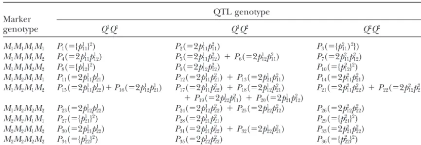
Table 1 describes a matrix for the population

frequen-ᏽl_{is expressed as}

cies of 27 zygote genotypes at two markers and one QTL, which contain 36 zygote configurations through random combinations of the eight haplotypes. As shown

Haplotype frequency Dsl

rk₁rk₂⫽p

sl

rk₁rk₂

3 disequilibria ⫺pslD

rk1rk2⫺prk2D

sl

rk₁⫺prk1D

sl

rk₂

No disequilibrium ⫺prk₁prk₂p

sl,

in the table, we use P␰(␰ ⫽ 1, . . . , 36) to denote the

frequencies of different zygote configurations. Because different configurations may produce the same zygote

genotype when paternal and maternal gametes have with constraints兺uk₁

r_k 1⫽1

Dsl

r_k 1rk2⫽兺

uk₂

r_k 2⫽1

Dsl

rk1rk2⫽兺 v_l sl⫽1D

s_l rk1rk2⫽

TABLE 1

Joint zygote probabilities of the QTL genotypes and two-marker genotypes in terms of

zygote configurationsP␰(␰⫽1, . . . , 36)

QTL genotype Marker

genotype Q1_Q1 _Q1_Q2 _Q2_Q2

M1M1M1M1 P1(⫽{p111}2) P2(⫽2p111p211) P3(⫽{p211)2}) M1M1M1M2 P4(⫽2p111p112) P5(⫽2p111p212)⫹P6(⫽2p112p112) P7(⫽2p211p212) M1M1M2M2 P8(⫽{p112}2) P9(⫽2p112p212) P10(⫽{p212}2) M1M2M1M1 P11(⫽2p111p121) P12(⫽2p111p221)⫹P13(⫽2p121p112) P14(⫽2p211p221)

M1M2M1M2 P15(⫽2p111p122)⫹P16(⫽2p112p211) P17(⫽2p111p222)⫹P18(⫽2p112p221) P21(⫽2p211p222)⫹P22(⫽2p212p221) ⫹P19(⫽2p122p211)⫹P20(⫽2p121p212)

M1M2M2M2 P23(⫽2p112p122) P24(⫽2p112p222)⫹P25(⫽2p122p122) P26(⫽2p212p222) M2M2M1M1 P27(⫽{p121}2) P28(⫽2p121p221) P29(⫽{p221}2) M2M2M1M2 P30(⫽2p121p122) P31(⫽2p121p222)⫹P32(⫽2p122p212) P33(⫽2p221p222) M2M2M2M2 P34(⫽{p122}2) P35(⫽2p122p222) P36(⫽{p222}2)

The expression for the frequency of each zygote configuration due to random recombination of paternal and maternal gametes is given in parentheses (see the text).

probabilities of the QTL genotypes and the marker ge-Hexagenic linkage disequilibria between four marker

notypes on the basis of their zygote formation. We now nonalleles and two QTL nonalleles are expressed as

introduce a genetic model for characterizing the addi-Dsl1sl2

rk 1rk2rk3rk3

⫽ tive, dominant, and epistatic effects of QTL affecting a

quantitative trait. We useMatherandJinks’(1982)

nota-Haplotype frequency

tion to describe the epistasis, under which the genotypic psl1sl2

rk

1rk2rk3rk4 _{values for any two QTL (}ᏽl_1andᏽl_{2) are expressed as}

15 digenic disequilibria

⫺prk₃prk₄p sl₁psl₂Dr_k

1rk2⫺ . . .⫺prk₁prk₂prk₃prk₄D sl₁sl₂

20 trigenic disequilibria

⫺prk₄p sl₁psl₂D_r

k₁rk₂rk₃⫺. . .⫺prk₁prk₂prk₃D sl

1sl2 rk

4

Ql_1genotype

␮{s₁s⬘

1}{s2s⬘2}

Q1_Q1 Q1_Q2 Q2_Q2

     

Ql 2genotype

Q1_Q1 _Q1_Q2 _Q2_Q2 ␮ ⫹al₁⫹al₂⫹il₁l₂ ␮ ⫹al₁⫹dl₂⫹jl₁l₂ ␮ ⫹al₁⫺al₂⫺il₁l₂

␮ ⫹dl

1⫹al2⫹kl1l2 ␮ ⫹dl1⫹dl2⫹ll1l2 ␮ ⫹dl1⫺al2⫺kl1l2

␮ ⫺al₁⫹al₂⫺il₁l₂ ␮ ⫺al₁⫹dl₂⫺jl₁l₂ ␮ ⫺al₁⫺al₂⫹il₁l₂

s1ⱕs⬘1,s2ⱕs2⬘⫽1, 2

      , 15 quadrigenic disequilibria

⫺psl₁psl₂D_r

k₁rk₂rk₃rk₄⫺. . .⫺prk₁prk₂D sl₁sl₂ rk₃rk₄

6 pentagenic disequilibria

(4)

⫽

⫺psl₂Dsl1 rk₁rk₂rk₃rk₄⫺

. . .⫺prk₁D sl₁sl₂

rk₂rk₃rk₄ where ␮ is the overall mean; al1,al2,dl1, anddl2 are the

45 digenic⫻digenic disequilibria additive and dominant effects of the two QTL, respectively;

andil1l2,jl1l2,kl1l2, andll1l2 are the additive⫻additive,

addi-⫺prk3prk4p

sl1psl2Drk1rk2⫺. . .⫺prk1prk2prk3prk4D sl1sl2

tive⫻dominant, dominant⫻additive, and dominant⫻

60 digenic⫻trigenic disequilibria

dominant epistatic effects between the two QTL,

respec-⫺prk 1Drk2rk3D

sl 1sl2 rk

4

⫺. . .⫺psl 2D

sl 1 rk 4

Drk

1rk2rk3 tively.

15 digenic⫻quadrigenic disequilibria _{The phenotypic value of a quantitative trait due to these}

⫺Drk₁rk₂rk₃rk₄D sl

1sl2⫺. . .⫺Drk₁rk₂D sl

1sl2

rk₃rk₄ two putative QTL for individualifrom a random sample

of the population can be written as

10 trigenic⫻trigenic disequilibria

⫺Drk₁rk₂rk₃D sl₁sl₂ rk₄ ⫺

. . .⫺Dsl₁sl₂ rk₁

Drk₂rk₃rk₄

yi⫽

兺

s1ⱕs⬘₁ s2ⱕ

兺

␮{s₁s⬘₁}{s₂s⬘₂}_x

iS1S⬘1S2S⬘2⫹ei, (5)

15 digenic⫻digenic⫻digenic disequilibria

⫺Drk₁rk₂Drk₃rk₄D

sl₁sl₂⫺. . .⫺Dsl2 rk₁

Dsl₁ rk₄

Drk₂rk₃

wherexiS1S1⬘S2S⬘2is an indicator variable, defined as 1 if

individ-No disequilibrium

ualihas QTL genotypeQs1_Qs1⬘_Qs2_Qs2⬘_{and 0 otherwise, and}

⫺prk₁prk₂prk₃prk₄p sl₁psl₂,

eiis the residual error, distributed asN(0,␴2). It is

possi-ble that each QTL genotype has a different residual

with constraints兺uk1

r_k 1⫽1

Dsl1sl2 r_k

1rk2rk3rk4

⫽. . .⫽兺vl2 s_l

2⫽1

Dsl1sl2 r_k

1rk2rk3rk4

⫽0.

variance. Since there are nine QTL genotypes, nine independent genotypic values arrayed by {␮{s1s⬘1}{s2s⬘2}_}

1⫻9can

be defined as in (4). These nine genotypic values are QUANTITATIVE GENETIC MODEL

composed of nine unknown quantitative genetic

param-In the above section, we discussed the population eters: one overall mean (␮), two additive {al1,al2}, two

achieved by differentiating the log-likelihood with

re-kl1l2,ll1l2}. The nine genotypic values and residual variance

spect to⍀, which leads to

comprise a quantitative genetic parameter vector

ar-rayed by ⍀q ⫽ {␮{11}{11}, . . . , ␮{22}{22}, ␴2}, which can be

⳵

⳵⍀logL(y,M,g|⍀)⫽r₁兺ⱕr⬘r₂兺ⱕr⬘

2

冦

1

z{r₁r⬘

1}{r2r⬘2} ·␰

⳵ ⳵⍀P

logP␰

estimated by incorporating the population genetic properties of the QTL within a mapping framework.

For many outcrossing populations, the biallelic-QTL

⫹ _兺

n{r₁r⬘₁}{r₂r⬘₂} i⫽1 兺

36

␰⫽1

z{r₁r⬘

1}{r2r⬘2}i␰兺 sⱕs⬘

x{ss⬘}

␰ ⳵

⳵⍀q

logf{ss⬘}(yi)

冧

suf-ficient and should be extended to a multiallelic-QTL

(8) situation. Quantitative genetic models based on

multial-lelic inheritance have been well discussed in the litera- _{where z}

{r₁r⬘₁}{r₂r⬘₂} ·␰⫽ 兺 n{r

1r⬘1}{r2r⬘2}

i⫽1 z{r1r⬘1}{r2r⬘2}i␰. By letting the score

ture (seeCockerham1980).

(Equation 8) equal zero and solving the log-likelihood equation, we obtain the maximum-likelihood estimates (MLE) of the unknown parameters as

STATISTICAL MODEL

Likelihood of the complete data: In this QTL map- _pˆ1

11⫽

1

2n(2n1⫹n2⫹n4⫹n5⫹n11⫹n12⫹n15⫹n17)

ping study, marker data (M) and phenotype data (y)

for all n individuals randomly drawn from a natural

pˆ2 11⫽

1

2n(n2⫹2n3⫹n6⫹n7⫹n13⫹n14⫹n19⫹n21)

population are observed data, whereas zygote formation

modes,i.e.,zygote configurations (g), are unobservable

or missing data. The observed data alone are incomplete

pˆ1 12⫽

1

2n(n4⫹n6⫹2n8⫹n9⫹n16⫹n18⫹n23⫹n24)

data, which, along with the missing data, comprise the complete data. For simplicity, the statistical framework

is illustrated for the relatively simple two-marker/one- pˆ2

12⫽

1

2n(n5⫹n7⫹n9⫹2n10⫹n20⫹n22⫹n25⫹n26)

QTL model. This framework can be extended to consider a multiple-marker/multiple-QTL model, considering

pˆ1 21⫽

1

2n(n11⫹n13⫹n16⫹n20⫹2n27⫹n28⫹n30⫹n31)

multiple alleles at each locus. The likelihood function of the complete data given the unknown parameters

⍀ ⫽ (⍀p, ⍀q) is written, under the two-marker/one- _pˆ2

21⫽

1

2n(n12⫹n14⫹n18⫹n22⫹n28⫹2n29⫹n32⫹n33)

QTL model, as

pˆ1 22⫽

1

2n(n15⫹n19⫹n23⫹n25⫹n30⫹n32⫹2n34⫹n35)

L(y,M,g|⍀)⫽

兿

r₁ⱕr⬘1

兿

r₂ⱕr⬘2

兿

n_{r1r⬘1}{r 2r⬘2}

i⫽1

pˆ2 22⫽

1

2n(n17⫹n21⫹n24⫹n26⫹n31⫹n33⫹n35⫹2n36)

⫻

冤

_兺

␰⫽1

z{r1r⬘1}{r2r⬘2}i␰P␰

兺

x{ss_⬘}

␰ f{ss_⬘}(yi)

冥

␮{ss⬘}⫽

兺

兺

兺

n{r 1r⬘1}{r2r⬘2}

i⫽1

兺

␰⫽1z{r1r⬘1}{r2r⬘2}i␰x

{ss⬘} ␰ yi

兺

兺

兺

n{r 1r⬘1}{r2r⬘2}

i⫽1

兺

␰⫽1z{r1r⬘1}{r2r⬘2}i␰x

{ss_⬘} ␰

or

L(y,M,g|⍀)⫽

兿

r1ⱕr⬘1

兿

r2ⱕr⬘2

兿

n_{r1r1}{⬘r2r⬘2}

i⫽1

兿

␰⫽1 ␴

2⫽1

n_r

兺

1ⱕr⬘1

兺

r2ⱕr⬘2

兺

n{r₁r⬘

1}{r2r⬘2}

i⫽1

兺

␰⫽1

z{r1r⬘1}{r2r⬘2}i␰

兺

sⱕs⬘

x{ss_⬘}

␰ (yi⫺ ␮ˆ{ss⬘})2,

⫻

冤

兺

sⱕs_⬘

x{ss_⬘} ␰ f{ss_⬘}(yi)

冥

z_{r 1r⬘1}{r2r⬘2}i␰

, (7)

wheren␰⫽ 兺r₁ⱕr⬘₁ 兺r₂ⱕr₂⬘z{r₁r⬘₁}{r₂r⬘₂}·␰denotes the sample size

of a particular zygote configuration␰(␰ ⫽1, . . . , 36)

as defined in Table 1. For the complete data,␰is

observ-wheren{r₁r⬘₁}{r₂r⬘₂}is the observed number of individuals with

able. Based on the invariance property of maximum-marker genotypeMr₁Mr⬘₁Mr₂Mr⬘₂,

likelihood estimates, the MLEs of allelic frequencies, the coefficients of linkage disequilibrium, and QTL ef-z{r1r⬘1}{r2r⬘2}i␰⫽

冦

1 if individualiwithin incomplete category Mr₁Mr⬘₁Mr₂Mr⬘₂

belongs to complete category␰(␰ ⫽1, . . . , 36)

0 otherwise

fects can be obtained from

aˆ⫽1

2(␮

{11}⫺ ␮{22}₎

x{ss⬘}

␰ ⫽

冦

1 if the QTL genotype of zygote formation␰is from

categoryQs_Qs_⬘(␰僆{Qs_Qs_⬘})

0 otherwise, _dˆ⫽ ␮{12}⫺ 1

2(␮

{11}⫹ ␮{22}₎

andf{ss⬘}(yi) is a normal density of observationyi with a pˆ_1(k

1)⫽pˆ

1

11⫹pˆ112 ⫹pˆ112⫹ pˆ212

particular QTL genotype Qs_Qs⬘_{having mean} ␮{ss⬘} _and

pˆ1(k₂)⫽pˆ111⫹pˆ112 ⫹pˆ121⫹ pˆ221

qˆ1 ⫽_pˆ1

11⫹pˆ112⫹ pˆ121⫹pˆ122 _⫻

冤

⳵⍀p

logP␰⫹

兺

sⱕs⬘ xss_␰⬘ ⳵

⳵⍀q

logf{ss⬘}(yi)

冥

Dˆl

k₁ ⫽pˆ111⫹ pˆ121 ⫺pˆ1(k₁)qˆ1 ₍₁₀₎

Dˆl

k₂ ⫽pˆ111⫹ pˆ211 ⫺qˆ1pˆ1(k₂) _where

Dˆk₁k₂ ⫽pˆ111⫹ pˆ211⫺pˆ1(k₁)pˆ1(k₂)

⌸{r1r⬘1}{r2r⬘2}i␰⫽

w{r₁r⬘₁}{r₂r⬘₂}␰P␰

兺

␰ f{ss_⬘}(yi)

兺

␰⫽1

关

兺

␰ f{ss⬘}(yi)

兴

, Dˆl

k1k2⫽pˆ 1

11⫺ pˆ1(k₁)Dˆlk₂ ⫺pˆ1(k₂)Dˆlk₁⫺qˆ1Dˆk₁k₂ ⫺pˆ1(k₁)qˆ1pˆ1(k₂).

(11)

The likelihood of incomplete data:The data of QTL

mapping are incomplete because only marker data and

which could be thought of as a posterior probability that phenotype data can be observed and the data on zygote

individualihas a marker-QTL zygote configuration␰given

configurations and QTL genotypes are missing. The

marker zygote genotype G{r₁r⬘₁}{r₂r₂⬘}. We then implement

likelihood of incomplete data is built upon a mixture

the EM algorithm (Dempster et al. 1977) with the

ex-model in that each individual is assumed to have arisen

panded parameter set {⍀, ⌸}, where⌸⫽{⌸{r1r⬘1}{r2r2⬘}i,i⫽

from one of these unknown QTL genotypes. Finite

mix-1, . . . ,n{r1r⬘1}{r2r⬘2};r1ⱕr⬘1,r2ⱕr2⬘⫽1, 2}.

tures of distributions used to model a wide variety of

Each iteration consists of two steps. First, on the E

random phenomena (seeMcLachlanandPeel2000)

step, the complete-data log-likelihood is averaged over can provide a sound mathematical-based approach for

the conditional distribution of the indicator variables distinguishing unknown QTL genotypes. With a normal

given the observed data, using the current estimate of mixture model-based approach for separating QTL

ge-the parameter vector. Since ge-the complete-data log-likeli-notypes, the likelihood function of incomplete data

in-hood is linear in these indicator variables, the E-step of

cluding the phenotype (y) and marker information (M)

is written as the EM algorithm involves simply replacing them by the

current values of their conditional expectations, that is, L(y,M|⍀)⫽

兿

r1ⱕr⬘1

兿

兿

i⫽1

the posterior probabilities of component membership expressed in Equation 11. Next, in the M step,

condi-tional on⌸, we solve for the zeros of Equation 10

(likeli-⫻

冦

兺

␰⫽1

冤

P␰|{r₁r⬘₁}{r₂r⬘₂}

兺

sⱕs_⬘

x{_␰ss⬘}f{ss_⬘}(yi)

冥冧

hood equations) to get our estimates of⍀. The

likeli-hood equation can be split into two terms: The first term refers to the genetic association as specified by

⫽

_兿

r1ⱕr⬘1

兿

兿

i⫽1

冦

兺

36

␰⫽1

冤

w{r₁r⬘₁}{r₂r⬘₂}␰P␰

兺

sⱕs⬘ x{ss⬘}

␰ f{ss_⬘}(yi)

冥冧

haplotype frequencies, and the second term to the phe-notype-genotype relationship described by the

geno-where Prob(G{r₁r⬘₁}{r₂r⬘₂}) is the population frequency of

typic means and residual variance. The estimates are marker genotypes at the two markers,

then used to update⌸ in the E step, and the process

is repeated until convergence. The values at conver-w{r1r⬘1}{r2r⬘2}␰⫽

冦

1 if complete category␰is compatible

to marker categoryMr1Mr⬘1Mr2Mr⬘2

0 otherwise

gence are the MLEs.

It is interesting to note that the estimation of allelic frequencies and coefficients of linkage disequilibria can

and the other notation is defined as above. _{be obtained from the closed-form solutions of haplotype}

The estimation of haplotype frequencies is based on _{frequencies. This will largely improve the computational}

the number of a particular haplotype in the population. _{efficiency of these parameters that can only be}

ex-For the complete data, 36 modes of zygote formation _{pressed as polynomial equations using traditional}

proce-via random combinations of paternal haplotypes and

dures (seeLuoandSuhai1999;Luoet al.2000;Wuet

maternal haplotypes are knowna prioriand, therefore,

al.2002).

the number of various marker-QTL haplotypes can be

Disequilibrium mapping of epistatic QTL: We

con-directly counted (see Table 1). But for the incomplete

sider two cases for mapping QTL with epistasis for a data, zygote formation is unobservable and its inference

quantitative trait based on linkage disequilibrium. First, is viewed as a missing data problem. In fact, it is possible

two epistatic QTL are predicted by two independent to calculate the expected number of a particular

marker-pairs of markers. Second, two epistatic QTL are pre-QTL haplotype for a given marker zygote genotype.

dicted by two pairs of genetically associated markers. Although marker-QTL zygote genotypes are also

un-In the first case, the two QTL can be assumed to be known, they can be inferred on the basis of marker

independent from a population genetic standpoint, al-information and phenotype data by implementing the

though they are not so in terms of quantitative genetic EM algorithm. By differentiating Equation 9, we have

effects. In the second case, the two QTL should be associated genetically and interact epistatically to affect

⳵

⳵⍀logL(y,M|⍀)⫽r1ⱕ

兺

兺

兿

n{r₁r⬘₁}{r₂r⬘₂}

i⫽1

兺

proposed for the above two-marker/one-QTL model is when some regularity conditions are violated. The

per-mutation test approach proposed by Churchill and

extended to estimate both population and quantitative

genetic parameters. Doerge(1994), which does not rely upon the

distribu-tion of the LRQ, may be used to determine the critical

Two basic tasks should be completed before the

im-plementation of the EM algorithm for epistasis map- threshold for claiming the existence of a QTL.

After the existence of the QTL is statistically tested,

ping. The first task is the derivation of an (81 ⫻ 9)

matrix for joint probabilities of four-marker/two-QTL we formulate a second test for its association with two

markers under consideration. The log-likelihood ratio zygote genotypes based on zygote configurations. For

two independent sets of markers and QTL, such proba- for such a test is calculated by

bilities are simply calculated as the Krockner product

LRQ

of the joint probability for each set, so that there are 16

haplotype frequencies (and 14 independent haplotype ⫽ ⫺2 log

冤

s_,Dˆ k1k2,Dˆ

s k1⫽Dˆ

s k2⫽Dˆ

s k1k2⫽0,⍀

˜_q,␴˜2₎

L(y,M|⍀ˆp,⍀ˆq,␴ˆ2)

冥

,

frequencies) in this case. But for two dependent sets of

loci, the derivations of such probabilities should con- (14)

which is asymptotically distributed as a␹2 _distribution

sider the formation principle of a six-locus zygote, in

with 3 d.f. which case there are a total of 64 haplotype frequencies,

Other more specific tests for the existence of additive, of which 63 are independent. In the first case, we have

dominant, or epistatic effect and the association of a only digenic and trigenic linkage disequilibria, whereas,

QTL with a particular marker can also be formulated in the second case, we must face digenic, trigenic,

quad-similarly. Generally, these hypotheses can be tested on rigenic, pentagenic, and hexagenic disequilibria (see

the basis of a critical threshold calculated from permuta-Equation 3).

tion tests (Churchill and Doerge 1994). Other

ap-The second task is the modeling of epistatic QTL with

proaches as proposed by Piepho (2001) can also be

additive, dominant, and additive⫻additive, additive⫻

used, which do not require expensive computations.

dominant, dominant⫻additive, and dominant⫻

domi-nant interaction effects (see matrix 4). The estimation of both population (from the first task) and quantitative

MONTE CARLO SIMULATION genetic parameters (from the second task) for epistatic

QTL can be obtained using closed forms. Simulation scenarios: We have performed extensive

simulation studies to investigate the robustness and

per-Hypothesis tests: We can test two major hypotheses

in the following sequence: (1) the existence of QTL formance of our linkage disequilibrium-based mapping

of quantitative traits. A number of simulation scenarios by testing the significance of QTL effects and (2) the

association of significant QTL with markers by testing are performed to compare results under different QTL

models (one-marker/one-QTL vs. multiple-marker/

linkage disequilibrium. The test for the existence of

a significant QTL may not rely upon the association multiple-QTL), different heritability levels, different

sample sizes, and different population genetic parame-between the QTL and known marker(s), but the

ran-dom association of a QTL with markers can be tested ters (equal vs. extreme allele frequencies at a locus).

Marker and QTL genotype data are simulated on the only when the existence of the QTL is statistically tested.

The existence of a QTL can be tested on the basis of basis of joint frequencies for a given sample size, whereas

phenotype data are simulated by summing genotypic two alternative hypotheses:

values and environmental errors, distributed asN(0,␴2_).

H0:␮{11}⫽ ␮{12} ⫽ ␮{22} _{The residual variance}␴2_{is determined under a given}

heritability level. The simulated data are analyzed using

H1: at least one equality does not hold. (12)

the genetic model proposed in this article. Each

simula-The log-likelihood-ratio test statistic for the existence _{tion scenario was repeated 200 times to estimate the}

of a QTL is calculated by comparing the likelihood _{biases and mean square errors of the MLEs.}

values under H1(full model) and H0(reduced model), _{To show the advantage of our multilocus}

disequilib-using _{rium model, we first perform the analysis on the basis of}

a one-marker/one-QTL model (MQ), as used in earlier

LRQ⫽ ⫺2 log

冤

L(y,M|⍀˜_p,␮{11}_{⫽ ␮}{12}_{⫽ ␮}{22}_,␴

˜2)

L(y,M|⍀˜p,⍀˜q,␴ˆ2)

冥

, (13) _{studies (LuoandSuhai1999;Luoet al. 2000;Wuet al.}

2002). The results from MQ are compared with those

where the tilde denotes the MLEs of unknown parame- obtained from a two-marker/one-QTL model (MQM)

ters under H0and the other notation is defined as above. and two epistatic QTL models (two separate sets of

two-The LRQis considered to asymptotically follow a␹2distri- marker/one-QTL models, denoted by MQM-MQM, and

bution with the degrees of freedom equaling the dif- two dependent sets of two-marker/one-QTL models,

ference of the number of unknown parameters to be denoted by MQMMQM). For each QTL model, we

de-estimated under the two hypotheses. However, the ap- sign two different heritabilities (H2⫽_{0.1 vs.0.4), two}

different sample sizes (n⫽500vs.1000), and two

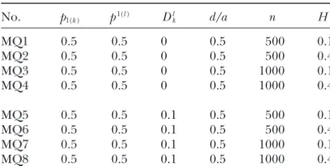
TABLE 2 mapping (MQM5–MQM8; Table 6) over disequilibrium mapping (MQ5–MQ8; Table 5).

Experimental designs of linkage disequilibrium mapping

We also design a scheme in which two markers are based on the one-marker/one-QTL model (MQ)

associated with each other, both of which are further

No. p1(k) p1(l) Dlk d/a n H2 associated with a putative QTL (MQM9–MQM12).

Al-though this kind of mutual association may not lead to

MQ1 0.5 0.5 0 0.5 500 0.1

a significant improvement for the MLEs of QTL allele

MQ2 0.5 0.5 0 0.5 500 0.4

frequency and residual variance, the estimation for the

MQ3 0.5 0.5 0 0.5 1000 0.1

model mean, the additive and dominant effects of the

MQ4 0.5 0.5 0 0.5 1000 0.4

QTL, and the residual variance is largely benefitted by

MQ5 0.5 0.5 0.1 0.5 500 0.1 _{a simultaneous use of two associated markers (MQM9–}

MQ6 0.5 0.5 0.1 0.5 500 0.4

MQM12; Table 6).

MQ7 0.5 0.5 0.1 0.5 1000 0.1

We examine the effects of different allelic frequencies

MQ8 0.5 0.5 0.1 0.5 1000 0.4

on parameter estimation. The relative frequencies of two alternative alleles reveal the degree of genetic differ-entiation in a population. When QTL alleles are less

ent allele frequencies for a locus. These designs includ- _{differentiated, as shown by the allele frequencies of}

ing the hypothesized parameter values are listed in Ta- _{0.3vs.0.7 (MQM13–MQM16), the precision of the MLEs}

bles 2–4. _{is not affected as long as more differentiated markers}

Results:Compared to the excellent accuracy and pre- _{are used (Table 6). We also found that the inclusion of}

cision of the MLEs of marker allele frequencies that _{some less differentiated markers did not affect the MLEs}

were obtained directly from the observed data, the accu- _{of QTL parameters (MQM17–MQM20). However, when}

racy and precision of the MLEs of QTL-allele frequency _{less differentiated markers are used to predict less}

differ-and disequilibrium differ-and QTL effects are relatively re- _{entiated QTL (MQM21–MQM24), the estimation}

preci-duced, sometimes seriously. As expected, the MLEs of _{sion of QTL effects and model parameters is largely}

QTL-related parameters under all given QTL models _{affected, although this may not be true for the MLEs}

from MQ to MQMMQM (Table 2–4) display increased _{of the population genetic parameters of QTL.}

accuracy and precision with increased heritabilities and

Additive-dominant-epistasis model:When two QTL

inter-sample sizes, although the extent of the increase may

act epistatically, we develop two different multilocus be different among the models (Table 5–7). Generally, a

disequilibrium schemes to estimate their epistasis. The more significant improvement of parameter estimation,

first scheme (MQM-MQM) permits simultaneous use of especially for QTL allele frequency and disequilibrium,

two independent sets of markers to predict their

corre-was observed whenH2_{is increased from 0.1 to 0.4 than}

sponding QTL, whereas the second scheme (MQMMQM)

whenNis increased from 500 to 1000.

assumes two dependent sets of marker-QTL

relation-Additive-dominant model:Under MQ, we consider two

ships. In general, more tightly linked loci tend to have situations, one with no disequilibrium between the

a greater chance for nonrandom association than less marker and QTL (MQ1–MQ4) and the other with

dis-tightly linked loci do. Thus, the first scheme is roughly equilibrium between the two loci (MQ5–MQ8). The

similar to a situation in which two sets of markers and first situation is similar to the detection of major genes

QTL are from different chromosomes, whereas the sec-because marker information is actually not used. It is

ond scheme is similar to a situation in which two sets found that the MLEs of all QTL-related parameters in

of loci are from the same chromosome. the second situation are improved over those in the first

In the first scheme, all genetic parameters can be situation, especially for the dominant effect of the QTL

estimated with reasonable accuracy and precision (Ta-and model mean (Table 5), suggesting the value of

ble 7), suggesting that our disequilibrium-based map-utilizing marker information in quantitative genetic

re-ping strategy can be used to map epistatic QTL. When search.

two independent marker pairs are used at the same In MQM, we first assume that both markers are not

time, the MLEs of allele frequencies and QTL-associated with a putative QTL (MQM1–MQM4). As

marker disequilibrium are more precise than when only expected, this has no improvement in parameter

estima-one marker pair is used. The root mean-square errors of tion compared to MQ1–MQ4 (Table 6). Second, we

these estimates areⵑ0.122 for QTL allele frequencies,

assume that one of the two markers is associated with

0.033 for QTL-marker digenic disequilibrium, and 0.017 the QTL (MQM5–MQM8), whereas the second marker

for QTL-marker trigenic disequilibrium under MQM-is not. ThMQM-is design MQM-is similar to composite interval

map-MQM1 when two independent marker sets are used ping in which those markers outside the marker interval

(Table 7). Yet, the corresponding values are 0.161, carrying a QTL are used as cofactors to control genome

0.045, and 0.023 under MQM9 when one marker pair background. We did not observe any improvement in

TABLE 3

Experimental designs of linkage disequilibrium mapping based on the two-marker/one-QTL model (MQM)

No. p1(k1) p1k2 p

1(l) _Dk

1k2 D

l

k1 D

l

k2 D

l

k1k2 d/a n H

2

MQM1 0.5 0.5 0.5 0 0 0 0 0.5 500 0.1

MQM2 0.5 0.5 0.5 0 0 0 0 0.5 500 0.4

MQM3 0.5 0.5 0.5 0 0 0 0 0.5 1000 0.1

MQM4 0.5 0.5 0.5 0 0 0 0 0.5 1000 0.4

MQM5 0.5 0.5 0.5 0 0.1 0 0 0.5 500 0.1

MQM6 0.5 0.5 0.5 0 0.1 0 0 0.5 500 0.4

MQM7 0.5 0.5 0.5 0 0.1 0 0 0.5 1000 0.1

MQM8 0.5 0.5 0.5 0 0.1 0 0 0.5 1000 0.4

MQM9 0.5 0.5 0.5 0.1 0.1 0.1 0.04 0.5 500 0.1

MQM10 0.5 0.5 0.5 0.1 0.1 0.1 0.04 0.5 500 0.4

MQM11 0.5 0.5 0.5 0.1 0.1 0.1 0.04 0.5 1000 0.1

MQM12 0.5 0.5 0.5 0.1 0.1 0.1 0.04 0.5 1000 0.4

MQM13 0.5 0.5 0.3 0.1 0.1 0.1 0.04 0.5 500 0.1

MQM14 0.5 0.5 0.3 0.1 0.1 0.1 0.04 0.5 500 0.4

MQM15 0.5 0.5 0.3 0.1 0.1 0.1 0.04 0.5 1000 0.1

MQM16 0.5 0.5 0.3 0.1 0.1 0.1 0.04 0.5 1000 0.4

MQM17 0.3 0.5 0.5 0.1 0.1 0.1 0.04 0.5 500 0.1

MQM18 0.3 0.5 0.5 0.1 0.1 0.1 0.04 0.5 500 0.4

MQM19 0.3 0.5 0.5 0.1 0.1 0.1 0.04 0.5 1000 0.1

MQM20 0.3 0.5 0.5 0.1 0.1 0.1 0.04 0.5 1000 0.4

MQM21 0.3 0.3 0.3 0.1 0.1 0.1 0.04 0.5 500 0.1

MQM22 0.3 0.3 0.3 0.1 0.1 0.1 0.04 0.5 500 0.4

MQM23 0.3 0.3 0.3 0.1 0.1 0.1 0.04 0.5 1000 0.1

MQM24 0.3 0.3 0.3 0.1 0.1 0.1 0.04 0.5 1000 0.4

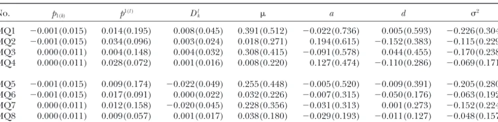
precision of QTL additive and dominant effects is re- dominant or dominant⫻additive interaction effect is

similar to the dominant effect, but the dominant ⫻

duced for MQM-MQM (Table 7).

In terms of estimation precision, more precise MLEs dominant interaction effect is poorer than the

domi-nant effect (Table 7). As expected, the MLE of the

of the additive ⫻ additive interaction effect between

two different QTL than those for the additive effect dominant⫻ dominant interaction effect may be quite

imprecise. However, when both sample size and

herita-at a single QTL are obtained, whereas the additive⫻

TABLE 4

Experimental designs of linkage disequilibrium mapping based on two independent sets of two markers and one QTL (MQM-MQM)

No. QTL p1(k1) p1k2 p

1(l) _Dk

1k2 D

l k1 D

l k2 D

l

k1k2 d/a i12/a j12/a k12/a l12/a H

2 _n

MQM-MQM1 1 0.5 0.5 0.5 0.1 0.1 0.1 0.04 0.5

0.2 ⫺0.2 0.2 ⫺0.2 0.1 500

2 0.5 0.5 0.5 0.1 0.1 0.1 0.04 0.5

MQM-MQM2 1 0.5 0.5 0.5 0.1 0.1 0.1 0.04 0.5

0.2 ⫺0.2 0.2 ⫺0.2 0.4 500

2 0.5 0.5 0.5 0.1 0.1 0.1 0.04 0.5

MQM-MQM3 1 0.5 0.5 0.5 0.1 0.1 0.1 0.04 0.5

0.2 ⫺0.2 0.2 ⫺0.2 0.1 1000

2 0.5 0.5 0.5 0.1 0.1 0.1 0.04 0.5

MQM-MQM4 1 0.5 0.5 0.5 0.1 0.1 0.1 0.04 0.5

0.2 ⫺0.2 0.2 ⫺0.2 0.4 1000

TABLE 5

Biases (and squared roots of mean square errors) of genetic parameter estimates based on the one-marker/one-QTL model (MQ)

No. p1(k) p1(l) Dlk ␮ a d ␴2

MQ1 ⫺0.001(0.015) 0.014(0.195) 0.008(0.045) 0.391(0.512) ⫺0.022(0.736) 0.005(0.593) ⫺0.226(0.304)

MQ2 ⫺0.001(0.015) 0.034(0.096) 0.003(0.024) 0.018(0.271) 0.194(0.615) ⫺0.152(0.383) ⫺0.115(0.229)

MQ3 0.000(0.011) 0.004(0.148) 0.004(0.032) 0.308(0.415) ⫺0.091(0.578) 0.044(0.455) ⫺0.170(0.238)

MQ4 0.000(0.011) 0.028(0.072) 0.001(0.016) 0.008(0.220) 0.127(0.474) ⫺0.110(0.286) ⫺0.069(0.171)

MQ5 ⫺0.001(0.015) 0.009(0.174) ⫺0.022(0.049) 0.255(0.448) ⫺0.005(0.520) ⫺0.009(0.391) ⫺0.205(0.280)

MQ6 ⫺0.001(0.015) 0.017(0.091) 0.000(0.022) 0.032(0.226) ⫺0.007(0.315) ⫺0.050(0.176) ⫺0.063(0.192)

MQ7 0.000(0.011) 0.012(0.158) ⫺0.020(0.045) 0.228(0.356) ⫺0.031(0.313) 0.001(0.273) ⫺0.152(0.224)

MQ8 0.000(0.011) 0.009(0.057) 0.001(0.017) 0.038(0.180) ⫺0.029(0.193) ⫺0.011(0.127) ⫺0.048(0.157)

bility are significantly increased, the MLEs of the domi- polymorphisms (SNPs) were genotyped at six candidate

genes for obesity on different chromosomes, which are

nant⫻dominant effect can be close to those of other

parameters (Table 7). ADRB1,ADRB2, ADRB3, ADRA1A, the GSprotein␣

-sub-unit (GNAS1), and the G protein ␤3 subunit (GNB3;

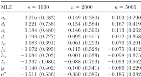
In the second scheme, the precision of the MLEs of

all parameters is reduced, compared to the first scheme, J. A.Johnson,unpublished results). TheADRB1 gene

contains two common nonsynonymous polymorphisms because of the inclusion of many unknowns. We

per-form an additional simulation underH2⫽ _{0.4 for the at codon 49 (Ser}→_{Gly) and codon 389 (Arg}→_Gly).

At theADRB2 gene, there are three polymorphism sites

second scheme by increasing the sample size from 1000

to 2000 to 5000, keeping the other parameters un- at codon 19 of the␤2AR 5⬘leader cistron (Cys→Arg),

codon 16 (Gly→Arg), and codon 27 (Gln→Gly). Two

changed. The precision of the MLEs of population

ge-netic parameters remained approximately constant with sites at codon 131 and codon 371 were genotyped for

theGNAS1 gene.

increased sample sizes (data not given), but the MLEs

of gene effects including the additive, dominant, and Our newly developed statistical method is used to

perform the association studies between SNPs and body epistatic effects displayed significantly improved

preci-sion when the sample size is increased (Table 8). When heights in two different populations. According to

Mackay (2001), the gene for a quantitative trait

de-N⫽2000, the estimation of the additive and additive⫻

additive interaction effects achieves acceptable preci- tected by a SNP is called a quantitative trait nucleotide

sion under the complex MQMMQM model. The estima- (QTN). We found different QTN that affect human

tion of the other effects is certainly acceptable when a body heights between the black and white populations

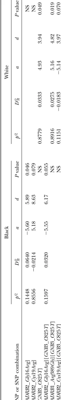
sample size is 5000 (Table 8). (Table 9). Two SNPs, Gly16Arg andCys19Arg, at gene

ADRB2 can identify significant QTN in the black

popula-tion, although the significance of the QTL detected by

A CASE STUDY FROM HUMANS _{the second SNP is marginal (Table 9). In fact, the QTL}

detected by these two SNPs may be identical for two A case study from a human genome project for

map-reasons. First, the sum of the allele frequencies of the ping obesity genes is used to validate our method. The

QTN identified is one, implying that variants detected subjects sampled consisted of 643 women from the

Na-by the two SNPs within the same gene are actually two tional Heart, Lung, and Blood Institute-funded

Wom-alternative alleles. This Wom-alternative relationship is con-an’s Ischemic Syndrome Evaluation (WISE) study ( J. A.

firmed by different signs of disequilibrium coefficients.

Johnson,unpublished results). Women included in the

Second, the QTN displays a similar genetic effect on

WISE study were⬎18 years old and consist of 105 blacks

body height, with different directions for the additive and 538 whites, each measured for body height and

effect as expected. This black-specific height QTN can other traits. However, as an example, only body height is

also be identified by combining one of these two SNPs analyzed here. All study participants provided informed

with SNPC825Tat geneGNB3.

written consent prior to participation in the study. WISE

In the white population, a significant QTN was de-study protocols were approved by the Institutional

Re-tected by SNPC835Tat geneGNB3 (Table 9). As shown

view Boards of the participants’ institutions.

by allele frequencies, linkage disequilibria, and genetic Genotypes for the women studied were determined

effects, we conjecture that the same QTN has been de-using Orchid BioScience’s proprietary primer extension

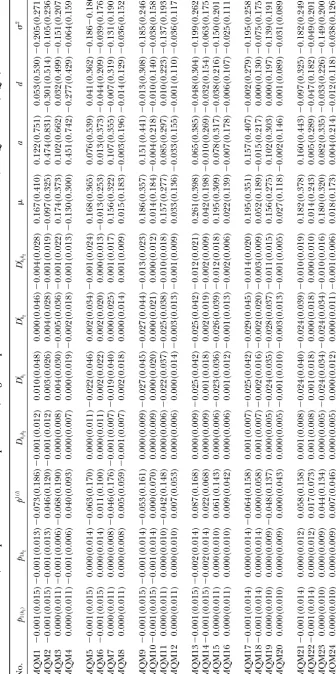
TABLE 6 Biases (and squared roots o f m ean square errors) of genetic parameter estimates based on the two-marker/one-QTL model (MQM) No. p1( k1 )

p1k

2 p 1( l ) Dk 1 k2 D

l k1

D

l k2

D

l kk1

TABLE 7 Biases (and squared roots o f mean square errors) of genetic parameter estimates based on two independent sets of two m arkers and one QTL (MQM-MQM) No. QTL p1( k1 )

p1k

2 p 1( l ) Dk 1 k2 D

l k1

D

l k2

D

l kk12