Statistical Issues in the Analysis of Quantitative Traits in Combined Crosses



Statistical Issues in the Analysis of Quantitative Traits in Combined Crosses

Fei Zou, Brian S. Yandell and Jason P. Fine

Department of Statistics, University of Wisconsin, Madison, Wisconsin 53706

Manuscript received August 14, 2000 Accepted for publication April 18, 2001

ABSTRACT

We consider some practical statistical issues in QTL analysis where several crosses originate in multiple inbred parents. Our results show that ignoring background polygenic variation in different crosses may lead to biased interval mapping estimates of QTL effects or loss of efficiency. Threshold and power approximations are derived by extending earlier results based on the Ornstein-Uhlenbeck diffusion process. The results are useful in the design and analysis of genome screen experiments. Several common designs are evaluated in terms of their power to detect QTL.

Q

UANTITATIVE trait analysis has many applica- several crosses, since the correlations may not be the tions in plant and animal breeding and in human same among all individuals. To avoid this difficulty, re-genetics. Mapping quantitative trait loci (QTL) that in- searchers may analyze data for each cross separately and fluence agriculturally important traits such as grain yield then compare and combine the results in some fashion. in rice or milk production in cows can help scientists Hence, some power to detect the QTL may be lost and produce specimens with more desirable qualities. Com- estimates of QTL effects may be less precise.

plex human diseases, like breast cancer and diabetes, Recently, methods were proposed to analyze all are known to have genetic etiologies. Animal models crosses simultaneously.Bernardo(1994) used Wright’s

may be useful in studying their origins. relationship matrixAto accommodate differential

cor-Most existing statistical methods have been developed relations when analyzing diallel crosses. However, when for experimental designs with a single cross from two closely related crosses are from a small number of in-inbred parents (Lander and Botstein 1989; Haley bred lines, it is more reasonable to treat the polygenic andKnott1992;Zeng1993, 1994; Jansenand Stam effect as fixed.Rebaiet al. (1994a) extended the regres-1994).Doergeet al.(1997) provided a comprehensive sion method ofHaleyandKnott(1992) to several F2’s review of methodologies for detecting and locating from a diallel design of multiple inbred lines with all genes affecting quantitative traits in experimental effects fixed.Elston(1990) proposed models for dis-breeding populations. However, quantitative traits are criminating among modes of inheritance, including often influenced by several genes with large effects (ma- one-locus, two-locus, polygenic, and mixed major locus/ jor QTL) and many genes with relatively small effects polygenic inheritance when considering the F1and the (polygenes). In animal science, where outbred parental reciprocal backcrosses derived from two inbred lines. populations are available, the polygenic effect has been The polygenic effect is treated as fixed and different taken into consideration (Fernando and Grossman phenotypic means and variances are used for different 1989). In horticulture, less attention has been paid to crosses. However, flanking marker information is not genes with small effects, perhaps because researchers utilized and an estimate of the QTL position is not are able to rely on simple crosses such as F2or backcross provided.

(BC). In this article, we consider an arbitrary number of

The effects of polygenes on standard approaches to crosses from multiple inbred lines. While we were pre-major QTL mapping are not well understood. With a paring this manuscript,LiuandZeng(2000) proposed single cross, the progeny have identical relationships a fixed-effect model to analyze combined crosses from given the QTL genotypes, resulting in a compound sym- multiple inbred lines (with or without overlapping in-metry structure (Yandell1997, Ch. 25). Thus, unbiased bred lines). Our model includes both QTL and poly-estimates of QTL effects are still obtained when the genic effects and is a special case of their heteroscedastic polygenic effect is ignored, even though the power to model in the sense that the fixed effect and the variance detect the QTL is influenced by the magnitude of the component identify the polygenic effect. For this rea-polygenic effect. The situation is more complicated with son, we refer readers toLiu andZeng(2000) for the analysis of combined lines. Our focus is the practical implications of the polygenic effects for QTL mapping, specifically bias and efficiency. Furthermore, we calcu-Corresponding author: Fei Zou, Department of Statistics, 1210 W.

Dayton St., Madison, WI 53706. E-mail: [email protected] late threshold values for controlling the genome-wise

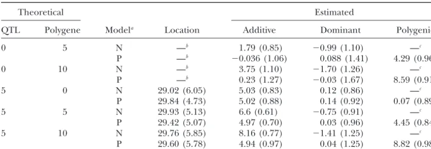
TABLE 1

Naivevs.polygenic model simulation

Theoretical Estimated

QTL Polygene Modela _{Location Additive Dominant Polygenic}

0 5 N —b _{1.79 (0.85)} ⫺_{0.99 (1.10) —}c

P —b ⫺_{0.036 (1.06) 0.088 (1.41) 4.29 (0.96)}

0 10 N —b _{3.75 (1.10) ⫺1.70 (1.26) —}c

P —b _{0.23 (1.27)} ⫺_{0.03 (1.67) 8.59 (0.91)}

5 0 N 29.02 (6.05) 5.03 (0.83) 0.12 (0.86) —c

P 29.84 (4.73) 5.02 (0.88) 0.14 (0.92) 0.07 (0.89)

5 5 N 29.93 (5.13) 6.6 (0.61) ⫺0.75 (0.91) —c

P 29.42 (5.07) 4.97 (0.70) 0.03 (0.96) 4.45 (0.84)

5 10 N 29.76 (5.85) 8.16 (0.77) ⫺1.41 (1.25) —c

P 29.60 (5.78) 4.94 (0.97) 0.04 (1.25) 8.82 (0.98) The values in parentheses are the standard deviations from 100 simulations. The numbers in the first two columns are the theoretical QTL and polygenic effects.

a_{N and P stand for the naive model and our polygenic model, respectively.} b_{The QTL position is not estimated since most of the max}

d{2 LR(d)}’s are not significant among 100

simulations.

c_{The polygenic effect is nonestimable in the naive model.}

type I error rate. Theoretical approximations were de- We observe that when there are no polygenes both models consistently estimate the QTL effects. However, veloped to address threshold and power (Landerand

Botstein 1989;DupuisandSiegmund 1999;Rebaiet model P gives more accurate estimates than model N when there are polygenic effects. The bias of model N al. 1994b, 1995) in some standard designs. However,

these methods are either impractical or inappropriate increases as the expected polygenic differences between BC1 and F2increase. In summary, our simulations indi-with combined crosses. Our general formulas are widely

applicable and easy to implement. cate that when analyzing combined crosses, the

poly-genic model produces more precise and less biased esti-mates than the traditional interval mapping method.

SIMULATION STUDY OF BIAS AND EFFICIENCY

If one combines different crosses simultaneously but

THRESHOLD AND POWER CALCULATIONS

ignores the different relationships among individuals,

substantial bias may result. In this section, we show the On the basis of the simulations in the above section, fitting combined crosses (LiuandZeng2000) has many effect of polygenes on the QTL estimates. We examine

two crosses, BC1 and F2, from common inbred parents advantages. Calculating thresholds and power is an im-portant practical issue in the design and analysis of such P1 and P2. Although the design is simple, it illustrates

the key issues. The additive effect of a single major QTL studies. The usual pointwise significance level based on the chi-square approximation is inadequate because the is set to 0 (i.e., no QTL) and 5, respectively, with no

dominance effect. Five markers are located at 0, 20, 40, entire genome is tested for the presence of a QTL.

LanderandBotstein(1989) showed that with an infi-60, and 80 cM. The major QTL is located at 30 cM. The

environmental errors are identically distributed for BC1 nitely dense map, the LOD score may be approximated in large samples by an Ornstein-Uhlenbeck diffusion and F2 and are sampled fromN(0, 25). One hundred

individuals from BC1 and F2are simulated without back- process for BC.Dupuis andSiegmund(1999) derived a similar result for F2. These approximations provide ground polygenes or with 10 background polygenes.

The 10 background polygenes are in coupling phase formulas for the threshold and power.

For more general models (LiuandZeng2000), no and have common additive effects (i.e., allele

substitu-tion effect␣k, k⫽1, 2, . . . , 10) 1 or 2 (seeFernando such approximation is available. Churchill and

Doerge(1994) used a randomization idea to calculate et al.1994). This leads to expected polygenic differences

between F2 and BC1 of 5 and 10, respectively. We fit the threshold. The approach is applicable for all de-signs, with a dense or sparse map. However, the method the model usingLiuandZeng(2000), hereafter called

“model P.” In addition, we employed traditional interval is computationally intensive. In addition, since the thresholds depend on the observed data, it is unclear mapping by ignoring the polygenic effects, hereafter

called “model N.” For each parameter combination, how to compare various designs. Rebai et al. (1994b, 1995) gave an upper bound for the threshold for BC 100 simulated datasets were analyzed. The results are

is formidable, even for an F2 population, and is not

H⫽

冢

0 0 0 1 0

0 0 0 0 1冣.

exact.Piepho(2001) proposed an efficient numerical method to compute the thresholds in Rebai et al.

From the normal regression theory, the likelihood ratio (1994b, 1995) for general designs.

statistic is Our approach extends the Ornstein-Uhlenbeck large

sample approximations. It is quite simple and practically

2 LR(d)⫽ ⫺nlog

冤

1⫺ (Hbˆ)⬘(H(X˜(d)⬘X˜(d))⫺1H⬘)⫺1(Hbˆ)

||y˜⫺X˜(d)bˆ||2_{⫹(Hbˆ)⬘(H(X˜(d)⬘X˜(d))}⫺1_H⬘)⫺1_(Hbˆ)

冥

,

useful. Calculating the threshold and power under dif-ferent map distances can be accomplished with

closed-wherey˜⫽ G⫺1/2_yandX˜(d)⫽_G⫺1/2_{X(d). UnderH} 0, form expressions arising from the Ornstein-Uhlenbeck

setup. Simulations shown below indicate this works well 2 LR(d)≈n(␦ˆ1␦ˆ2)(A22)⫺1(␦ˆ1␦ˆ2)⬘, with realistic sample sizes.

where (␦ˆ1 ␦ˆ2)⬘ is the maximum-likelihood estimate of Two inbred strains:In this section, we consider

com-b2⫽(␦1 ␦2)⬘andA22is given in (A2) in theappendix. bined crosses from two inbred parents (P1 and P2),

The distribution of 2 LR(d) depends on ␦ˆ1 and ␦ˆ2, BC1, F2, and BC2. Our goal is to extend Dupuis and

which are correlated. Thus, we cannot directly apply

Siegmund(1999). Generalizing the results to other

de-DupuisandSiegmund (1999) to derive the threshold signs (Liu and Zeng 2000) is straightforward. In the

and power. In theappendix, we propose an orthogonal sequel, we assume an equispaced marker map. Suppose

transformation such that 2 LR(d) is partitioned into the Y⫽(y11,y12, . . .y1n1;y21,y22, . . . ,y2n2;y31,y32, . . . ,y3n3)⬘ sum of squares of two uncorrelated random variables

Z1andZ2. This makes the asymptotic distribution

trans-⫽Xb⫹e⫽ (X1X2)

冢

b_b1

2

冣

⫹ e, parent. LettingWˆ1⫽ ␰1␦

ˆ_1,Wˆ_{2⫽ ␩1␦}ˆ_{1⫹ ␩2␦}ˆ_2(see

appen-dix for ␰1 and ␩i), Zi⫽

√

nWˆi, i ⫽ 1, 2. It is shown in theappendixthatZ1andZ2are asymptotically indepen-whereXis the design matrix andeis the random error.

dent and distributedN(0, 1). Thus, n1, n2,n3 are the number of observations for BC1, F2,

and BC2, respectively, withnobservations in total. The

submatrixX1 corresponds to the covariates identifying _{2 LR(d)}≈_n(Wˆ

1Wˆ2)

冢

W ˆ₁ Wˆ2

冣

⫽

n(Wˆ 2

1⫹Wˆ 22)⫽ Z21⫹ Z22, crosses or other measurements that do not involve the

QTL effects and X2 corresponds to the QTL effects.

which depends on two uncorrelated normal variates and Suppose the allele from parent P1 isqand from P2 is

is asymptotically␹2

2. Note that␦i,Wˆi, andZi,i⫽1, 2 all Q. The possible QTL genotypes are qq, Qq, and QQ.

depend on the locusd.In the sequel, when necessary, Ignoring other covariate effects, we let

we use␦1(d),␦2(d),Wˆi(d), andZi(d),i⫽1, 2 to emphasize their dependence ond.

To demonstrate the Ornstein-Uhlenbeck equiva-lence, the covariances at different loci d1 and d2 are proved to be

Cov(Z1(d1), Z1(d2))⫽1⫺ ␤1r⫹O(r2) X1⫽























1 1 0

. . .

1 1 0

1 0 0

. . .

1 0 0

1 0 1

. . .

1 0 1























and X2⫽























x111 x211 . . . . x11n1 x21n1

x121 x221 . . . . x12n2 x22n2

x131 x231 . . . . x13n3 x23n3























, and

Cov(Z2(d1), Z2(d2))⫽1⫺ ␤2r⫹O(r2).

This means that for largen,Z1(d) andZ2(d) are approxi-mately independent Ornstein-Uhlenbeck processes with mean zero and covariance 1⫺ ␤1r ⫹ O(r2) and wherex1ki⫽1 (or 0) if individualiin crosskhas genotype 1⫺ ␤_2r ⫹ _O(_r2), respectively. Adapting the argument Qq(or else), andx2ki⫽1 (or 0) if individuali in cross in_Dupuis and_Siegmund (1999), the tail distribution k has genotype QQ (or else). The random error e is _{of 2 LR under the null hypothesis satisfies}

normally distributed with mean 0 and Var(eki)⫽ ␴2k,i⫽

1, 2, . . . ,nk,k⫽ 1, 2, 3. In general Var(e)⫽ ␴23Gwith P(max

d 2 LR(d)ⱖa 2₎ G⫺1⫽_diag(␭

1, . . . ,␭1;␭2; . . . ,␭2; 1, . . . , 1), where␭k⫽

␴2

3/␴2kfork⫽1, 2. In the following, we assume that␭k

≈1⫺exp

⫺

冤

C⫹v(a(2␤⌬)

1/2_)a2_L

冢

␤1⫹ ␤2

2

冣冥

exp

冢

⫺

a2

2

冣

  ,

is known. If␭kis unknown, then consistent

maximum-likelihood (ML) estimates may be substituted and the ₍₁₎

result still holds. Without loss of generality, assume that

␴2

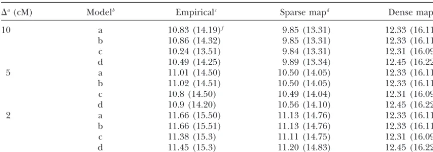
TABLE 2

95 and 99% critical LR threshold values

⌬a_{(cM) Model}b _Empiricalc _{Sparse map}d _{Dense map}e

10 a 10.83 (14.19)f _{9.85 (13.31) 12.33 (16.11)}

b 10.86 (14.32) 9.85 (13.31) 12.33 (16.11)

c 10.24 (13.51) 9.84 (13.31) 12.31 (16.09)

d 10.49 (14.25) 9.89 (13.34) 12.45 (16.22)

5 a 11.01 (14.50) 10.50 (14.05) 12.33 (16.11)

b 11.02 (14.51) 10.50 (14.05) 12.33 (16.11)

c 10.8 (14.50) 10.49 (14.04) 12.31 (16.09)

d 10.9 (14.20) 10.56 (14.10) 12.45 (16.22)

2 a 11.66 (15.50) 11.13 (14.76) 12.33 (16.11)

b 11.66 (15.51) 11.13 (14.76) 12.33 (16.11)

c 11.38 (15.3) 11.11 (14.75) 12.31 (16.09)

d 11.45 (15.3) 11.20 (14.83) 12.45 (16.22)

a⌬_{, the marker interval length. The length of chromosome is 100 cM.} b_{Sampled distributions of models a–d corresponding to BC1, F}

2, and BC2 populations, respectively, are a,

(N(1, 1),N(0, 1),N(⫺1, 1)); b, (N(0, 1),N(0, 1),N(0, 1)); c, (N(1, 1),N(0, 2),N(⫺1, 1)); d, (N(1, 2),N(0, 2),N(⫺1, 1)).

c_{The empirical thresholds are based on 5000 replications.}

d_{Sparse map calculation of the theoretical threshold based on (1).} e_{Dense map calculation using (1) withv⫽1 (i.e.,⌬ ⫽0).} f_{Thresholds at 95% (99%).}

be found inSiegmund(1985). For dense maps,v⫽1. 2, and models with covariates are also possible. Our

Similarly, the power is given by framework can be modified for a wide variety of designs.

As before, let the model be P(max

d 2 LRⱖa

2₎≈₁⫺ ⌽_(a⫺ ␻_*)⫹φ_(a⫺ ␻_*)

Y⫽Xb⫹e⫽ (X1X2)

冢

b_b1 2

冣

⫹e, ⫻

冤

1

2␻*⫹

2√av(a{2⌬␤}1/2₎

␻*3/2 ⫺

√av(a{2⌬␤}1/2₎2

␻*1/2_{(a⫹ ␻*)}

冥

whereX1is ann⫻ psubmatrix not involving the QTL when a QTL is located at a marker locus. Here

effects, X2 is ann ⫻ mmatrix corresponding to them QTL effects, andeis the random error. Following the v⫽ v(a{2⌬␤}1/2_),

procedure in theappendix, we first computeA22using (A2) and then derive the orthogonal transformation

␻*⫽

冪

nlog

冤

1⫹ ␰

2

1␦21⫹(␩1␦1⫹ ␩2␦2)2

␴2

BC

冥

,

matrixP from (A3). Note that bothA22and Pinvolve only the design matrix Xand not␤or the correlation parameters. Next, 2 LR(d) can be partitioned into the

␻*1 ⫽ ␻* ␰1␦1

√

␰2

1␦21⫹ (␩1␦1⫹ ␩2␦2)2 ,

sum of squares of masymptotically independent N(0, 1) random variables Z1, . . . , Zm, where Z ⫽ (Z1, . . . ,

␻*2 ⫽ ␻* ␩1␦1⫹ ␩2␦2

√

␰2

1␦21 ⫹(␩1␦1⫹ ␩2␦2)2

, _Z

m)⬘ ⫽Pbˆ2. To calculate Cov(Zj(d1),Zj(d2)),j⫽1, 2, . . . , m, we findDin (A4) on the basis of the specific designs. It is straightforward to establish

␤ ⫽ ␤1␻*12⫹ ␤2␻*22

␻*2 .

Cov(Zj(d1),Zj(d2))⫽1⫺ ␤jr⫹O(r2), j⫽1, 2, . . . ,m, For a QTL between markers, the noncentrality

param-where ␤j is thejth diagonal element of ⫺PA22DA⬘22P⬘. eters␻*1 and␻*2 are␻*1 exp(⫺␤1⌬1) and␻*2 exp(⫺␤2⌬1),

Now, the tail distribution of 2 LR under the null hypoth-respectively, where the distance between the QTL and

esis is approximately the marker is ⌬1. In the case of an F2 population, the

formulas above reduce to those in Dupuis and

Sieg-P(max

d

2 LR(d)ⱖ ␣2₎≈₁⫺_exp{⫺_C[1⫺ ␹2

m(␣2)] mund(1999).

General Results:The derivations above can be

gener-⫺v(a{2␤⌬}1/2_)␤L2(2⫺m)/2

alized to more complicated models, including those in

TABLE 3

Simulation of chromosome-wise type I error

⌬(cM) Model ␣ ⫽0.05 ␣ ⫽0.01

10 a 0.078 0.016

b 0.077 0.018

c 0.060 0.012

d 0.064 0.015

5 a 0.065 0.013

b 0.063 0.012

c 0.056 0.012

d 0.057 0.011

2 a 0.062 0.014

b 0.062 0.014

c 0.056 0.013

d 0.056 0.012

Models a–d are the same as in Table 2. The type I errors are calculated on the sparse map thresholds of the fourth column of Table 2.

where ␹2

m is a ␹2 random variable with m degrees of freedom and␤ ⫽(␤1⫹ ␤2 ⫹. . .⫹ ␤m)/m.

The formula for power may also be obtained. How-ever, it is quite complicated and is omitted here.

SIMULATION STUDY OF THRESHOLDS AND POWER

We investigated the performance of (1) with different marker distances and different polygenic backgrounds. Thresholds for the log-likelihood were based on interval

mapping with combined BC1, F2, and BC2 crosses.n1⫽ _{Figure 1.—(a) Additive QTL model. (b) Dominant QTL} n2 ⫽ n3 ⫽ 100, giving 300 observations in total and model. Power curves for equal BC1 and BC2 ratios under

dense maps. The horizontal line is the power calculated from

chromosome length ⫽ 100 cM. The marker interval

DupuisandSiegmund’s (1999) formula (i.e., the proportion

lengths are set at 10, 5, and 2 cM, respectively. Different

of F2 is 1). The lowest curve in a is the power when only polygenic effects are sampled, as reflected by models

available F2’s are used by discarding BCs. Thus power is re-a–d (see legend of Table 2 for details; Table 3). The _{duced because there are fewer individuals.}

approximations from (1) with v(a{2␤⌬}1/2_{) are always} smaller than the empirical thresholds derived in the

simulations. However, as the interval length decreases, tion should agree with DupuisandSiegmund (1999). Other noncentrality parameters in Dupuis and

Sieg-our approximations are more similar to the empirical

thresholds. In general, the dense map assumption (v⫽ mund(1999) show the same pattern and are omitted. For the additive model, the comparisons are qualita-1) produces conservative thresholds. Since more

mark-ers are likely to be typed around promising loci (Lander tively similar.

Figures 1 and 2 exhibit the power curves. When the and Kruglyak 1995), the stringent thresholds based

on a dense map should be used even with a sparse map. polygenes are in linkage equilibrium and have only addi-tive effects, the phenotypic variation due to polygenes Also, the approximations provide conservative control

of the genome-wise type I error rate. Note that (1) gives and environment satisfies ␴2

BC1 ⫽ ␴2BC2 ⫽ ␴2P ⫹ ␴2e and

␴F2⫽2␴2P⫹ ␴2e, respectively, where␴2Pis the total poly-upper and lower bounds for the threshold withv⫽ 1

(assuming a dense map) and withv(a{2␤⌬}1/2_{) (using genic variation in the BC population and}␴2

Pis the envi-ronmental variation. For this reason, we take ␭1 ⬅ 1 the true map distances), respectively.

Next, we evaluate the power with different propor- and choose␭⫺1

2 ⫽1, 0.75, 0.67, 0.57, 0.5, which corre-spond to␴2

P⫽0,␴2e/2,␴e2, 3␴2e, or␴2PⰇ ␴2e, respectively. tions of BC1, F2, and BC2. The power is calculated for

dominant (␦1⫽ ␦2) and additive (␦2⫽2␦1) models. We We also evaluate the power by using F2’s only, which quantifies the loss in power when discarding data from compare our results with those of Dupuis and

Sieg-mund(1999) for the dominant model. We use the same the BCs (see Figure 1a).

In Figure 1, the proportions of BC1 and BC2 are values of the noncentrality parameter. In theory, as the

Figure 2.—Power curves for different ratios of BC1, BC2, and F2 with dominant QTL under

dense maps. Dominant model with (a)␭2_{⫽1, (b)␭}2_{⫽0.75, (c)}

␭2_{⫽ 0.67, (d)␭}2 _{⫽0.5. a–d use}

the same graphical symbols. k1 is the sample proportion of BC1 and ␭2_{⫽ ␴}2

BC2/␴2F2.

gained by using BC populations unless there is no poly- QTL is additive, both BC1 and BC2 individuals have identical contributions in detecting the QTL, so only genic effect (i.e.,␭2 is close to 1). The larger the

poly-genic effects, the greater is the gain with BCs. However, the total proportion of BC1 and BC2 influences the power, as shown in Figure 1a.

when the QTL is additive, F2’s tend to have more infor-mation for detecting a QTL than do BCs, unless␴PⰇ

␴e(i.e., the polygenic effects are very large). Note that

CONCLUSION

when the proportion of F2 approaches 1, our results

again match those of Dupuis and Siegmund. In this article, we addressed some important practical

issues in the analysis of closely related crosses derived In Figure 2, we allow the proportions of BC1 and BC2

Piepho, H. P.,2001 A quick method for computing approximate ficient estimates of the QTL effects may occur if the

thresholds for quantitative trait loci detection. Genetics157:425– polygenic effect is ignored. We derived simple and gen- _432.

Rebai, A., B. Goffinet, B. ManginandD. Perret,1994a Detecting eral approximations for the threshold and power to

QTLs with diallel schemes, pp. 170–177 in Biometrics in Plant detect a QTL, allowing different designs to be

com-Breeding: Applications of Molecular Markers. 9th Meeting of the

EUCAR-pared. _{PIA, edited byJ. W. van OoijenandJansen.CPRO-DLO,}

Wagen-ingen, The Netherlands. Based on our power calculations, we find that the F2

Rebai, A., B. GoffinetandB. Mangin,1994b Approximate thresh-population is more robust in detecting QTL than the

olds of interval mapping tests for QTL detection. Genetics138:

two backcross populations. This confirmsLiuandZeng _235–240.

Rebai, A., B. GoffinetandB. Mangin,1995 Comparing power of (2000). Thus if the goal is to detect the QTL, then using

different methods for QTL detection. Biometrics51:87–99. a large F2population is highly recommended. However,

Siegmund, D.,1985 Sequential Analysis: Tests and Confidence Intervals. scientists may not be able to produce enough F2individ- Springer-Verlag, New York.

Yandell, B. S.,1997 Practical Data Analysis for Designed Experiments. uals or may for other reasons use different crosses. In

Chapman & Hall/CRC Press, London/Cleveland. this situation, analyzing all the data simultaneously is

Zeng, Z-B.,1983 Theoretical basis of separation of multiple link preferred. This strategy improves the power to detect _{gene effects on mapping quantitative trait loci. Proc. Natl. Acad.}

Sci. USA90:10972–10976. major QTL. In addition, this is an opportunity to detect

Zeng, Z-B.,1994 Precision mapping of quantitative traits loci. Genet-potential polygenic effects. The derivation of the

thresh-ics136:1457–1468. old approximation is easily extended to other designs

Communicating editor:Z-B. Zeng

beyond the combination of BC1, F2, and BC2. However, to our knowledge, the theoretical computation of thresholds involving multiple QTL is an open problem.

APPENDIX We thank anonymous reviewers for their critical reading of this

manuscript. This research was supported in part by the U.S.

Depart-In this section, for combined crosses from two inbred ment of Agriculture Hatch project through the University of

Wiscon-parents, we prove that the likelihood ratio 2 LR(d) can sin, College of Agricultural and Life Sciences.

be partitioned into the sum of the squares of two asymp-totically independent Ornstein-Uhlenbeck processes

LITERATURE CITED _{through an orthogonal transformation. Define}

Bernardo, R.,1994 Prediction of maize single-cross performance using RFLPs and information from related hybrids. Crop Sci.34:

B⫽lim n→∞

X˜(d)⬘X˜(d)

n ⫽

冢

B11 B12

B21 B22

冣

⫽

冢

X˜1X˜1 X˜1X˜2

X˜2X˜1 X˜2X˜2

冣

. (A1)

20–25.

Churchill, G. A.,andR. W. Doerge,1994 Empirical threshold

values for quantitative trait mapping. Genetics138:963–971. _{Note thatBdoes not depend on locusd.Let}

Davies, R. B.,1977 Hypothesis testing when a nuisance parameter is present only under the alternative. Biometrika64:247–254.

Davies, R. B.,1987 Hypothesis testing when a nuisance parameter _A⫽B⫺ _⫽

冢

A11 A12 A21 A22

冣

withA22⫽

冢

a1 a3

a3 a2

冣

is present only under the alternative. Biometrika74:33–43.

Doerge, R. W., Z-B. ZengandB. S. Weir,1997 Statistical issues in the search for genes affecting quantitative traits in experimental

populations. Stat. Sci.12:195–219. _C⫽ _A⫺1

22 ⫽

冢

c1 c3

c3 c2

冣

. (A2)

Dupuis, J.,andD. Siegmund,1999 Statistical methods for mapping quantitative trait loci from a dense set of markers. Genetics151:

373–386. Define

Elston, R. C.,1990 Models for discrimination between statistical alternative modes of inheritance, pp. 41–55 inAdvances in

Statisti-cal Methods for Genetic Improvement for Livestock, edited byD. Gia- _P⫽

冢

␰1 0

␩1 ␩2

冣

; thenPA22P⬘ ⫽

冢

1 0

0 1冣, (A3)

nolaandK. Hammond.Springer-Verlag, New York.

Fernando, R. L.,andM. Grossman,1989 Marker-assisted selection

using best linear unbiased prediction. Genet. Sel. Evol.21:467– _where␰₁ ⫽

√c

₁ ⫺_c2

3/c2, and␩1⫽c3/

√c

2,␩2 ⫽

√c

2.

477.

Making the orthogonal transformation

Fernando, R. L., C. StrickerandR. C. Elston,1994 The finite polygenic model: an alternative formulation for the

mixed-model of inheritance. Theor. Appl. Genet.88:573–580.

冢

Z1 Z2

冣

⫽P

冢

␦

ˆ₁

␦ˆ₂

冣

Haley, C. S.,andS. A. Knott,1992 A simple regression method for mapping quantitative trait in line crosses using flanking markers.

Heredity69:315–324. _gives

Jansen, R. C.,andP. Stam,1994 High resolution of quantitative traits into multiple quantitative trait in line crosses using flanking

markers. Heredity69:315–324. _lim

n→∞

Var(Z1)⫽ lim n→∞ n

Cov (␰1, 0)

冢

␦ˆ₁

␦ˆ₂

冣

, (␰1, 0)

冢

␦ˆ₁

␦ˆ₂

冣

   Lander, E. S.,andD. Botstein,1989 Mapping Mendelian factors

underlying quantitative traits using RFLP linkage maps. Genetics 121:185–199.

Lander, E. S.,andL. Kruglyak,1995 Genetic dissection of complex _{⫽ lim}

n→∞ n

(␰1, 0)Var

  

冢

␦ˆ₁

␦ˆ₂

冣

  

冢

␰

ˆ₁ 0冣 traits: guidelines for interpreting and reporting linkage results.

Nat. Genet.11:241–247.

Liu, Y.,andZ-B. Zeng, 2000 A general mixture model approach

For the same reason,

D⫽

冢

⫺ ␭1k1⫹ 2␭2k2⫹k3

2

␭2k2⫹k3 2

␭2k2 ⫹k3

2 ⫺ ␭

2k2⫹k3

2

冣

. lim

n→∞ Var(Z2)⫽(␩1,␩2)(HAH⬘)

冢

␩1

␩2

冣

⫽1

and

Thus,

lim

n→∞ Cov(Z1,Z2)⫽(␰1, 0)(HAH⬘)

冢

␩1

␩2

冣

⫽0. _Cov(bˆ(d

1),bˆ(d2))⫽Cov[(X˜(d1)⬘X˜(d1))⫺1X˜(d1)⬘y, (X˜(d2)⬘X˜(d2))⫺1X˜(d2)⬘y] This indicates thatZ1andZ2are approximately

indepen-dentN(0, 1). Furthermore,

≈ACov(X˜(d1)⬘y,X˜(d2)⬘y)A n2

2 LR(d)≈n(␦ˆ1␦ˆ2)(A22)⫺1(␦´1␦ˆ2)⬘

⫽ 1

n2AX˜(d1)⬘X˜(d2)A

⫽(␦ˆ1␦ˆ2)

冢

␰1 ␩1

0 ␩2

冣冢冢

␰1 0

␩1 ␩2

冣

A22

冢

␰1 ␩1

0 ␩2

冣冣

⫺1

冢

␰1 0

␩1 ␩2

冣冢

␦ˆ₁ ␦ˆ₂

冣

⫽(␦´1␦ˆ2)

冢

␰1 ␩1

0 ␩2

冣冢

␰1 0

␩1 ␩2

冣冢

␦ˆ₁ ␦ˆ₂

冣

⫽A

n ⫹

A

冢

0 0 0 D

冣

A

n r⫹

O(r2₎ n . ⫽n(Wˆ1Wˆ2)

冢

Wˆ1

Wˆ1

冣

⫽n(Wˆ 2

1⫹Wˆ 22)⫽Z21⫹Z22.

Therefore,

Now, letX˜(d1) andX˜(d2) be the corresponding trans- _{Cov(Z1(d1),Z1(d2))⫽nCov(W}ˆ₁(d1),Wˆ1(d2))

formed incidence matrices at loci d1 andd2. Note that the first and second columns ofX˜ depend only on the

⫽n(␰1, 0)HCov(bˆ(d1),bˆ(d2))H⬘

冢

␰1

0

冣

proportions of BC1, F2, and BC2 and not ond1andd2.

The third and fourth columns depend on d1 and d2.

⫽1⫹

冤

a2 1

冢

⫺ ␭

1k1⫹2␭2k2⫹k3

2

冣

⫹2a1a3

␭2k2⫹k3

2 Alsox1ki(d)⫽0, 1, or 0 andx2ki(d)⫽0, 0, or 1 if individual

iin crossK’s genotype at locusdisqq,Qq, orQQ,

respec-tively. _⫹a2

3

冢

⫺ ␭ 2k2⫹k3

2

冣冥

␰

2 1r⫹O(r2)

For BC1,

⫽1⫺ ␤1r⫹O(r2)

(x1ki(d1),x1ki(d2))⫽







(0,0) with probability (1⫺r)/2 (0,1) or (1,0) with probabilityr

(1,1) with probability (1⫺r)/2 and

Cov(Z2(d1),Z2(d2))⫽nCov(Wˆ2(d1),Wˆ2(d2))

(x1ki(d1),x2ki(d2))⫽

  

(0,0) with probability 1/2

(1,0) with probability 1/2,

⫽n(␩1,␩2)HCov(bˆ(d1),bˆ(d2))H⬘

冢

␩1

␩2

冣

where r is the recombination fraction between locid1

and d2. Enumerating the probabilities of (x1ki(d1), _⫽1⫹

冤

a2 1

冢

⫺ ␭1

k1⫹2␭2k2⫹k3

2

冣

⫹2a1a3

␭2k2⫹k3

2 x1ki(d2)), (x1ki(d1),x2ki(d2)), and (x2ki(d1),x2ki(d2)) for BC1,

F2, and BC2, and using the fact thatX˜(d)⫽G⫺1/2X(d),

⫹a2 3

冢

⫺ ␭2

k2⫹k3

2

冣冥

␩

2 1r

we obtain

lim

n→∞

X˜_⬘(d1)X˜(d2)

n ⫹

冤

a23

冢

⫺ ␭

1k1⫹2␭2k2⫹k3

2

冣

⫹2a3a2

␭2k2⫹k3

2

⫹a2 2

冢

⫺ ␭

2k2⫹k3

2

冣冥

␩

2 2r

⫽

冢

X˜_⬘1X˜₁ X˜_⬘1X˜₂

X˜_⬘2X˜₁ X˜_⬘2X˜_2⫹

冢

⫺ ␭1k1⫹2␭2k2⫹k3

2

␭2k2⫹k3

2

␭2k2⫹k3

2 ⫺ ␭

2k2⫹k3

2

冣

r⫹O(r2₎

冣

⫹2

冤

a1a3

冢

⫺ ␭

1k1⫹2␭2k2⫹k3

2

冣

⫹(a

2 3⫹a1a2)␭

2k2⫹k3

2

⫹a3a2

冢

⫺ ␭ 2k2⫹k3

2

冣冥

␩1␩2r⫹O(r

2₎

⫽B⫹

冢

0 0

0 D

冣

r⫹O(r

2_),

(A4)

⫽1⫺ ␤2r⫹O(r2).