Parameter estimation for random differential equation models

(1)

Parameter Estimation for Random Differential Equation Models

H.T. Banks and Michele L. Joyner

Center for Research in Scientific Computation

North Carolina State University

Raleigh, NC, United States

and

Dept of Mathematics and Statistics

East Tennessee State University

Johnson City, TN 37614

December 13, 2016

Abstract

We consider two distinct techniques for estimating random parameters in random differential equation (RDE) models. In one approach, the solution to a RDE is represented by a collection of solution trajectories in the form of sample deterministic equations. In a second approach we employ pointwise equivalent stochastic differential equation (SDE) representations for certain RDEs. Each of the approaches is tested using deter-ministic model comparison techniques for a logistic growth model which is viewed as a special case of a more general Bernoulli growth model. We demonstrate efficacy of the preferred method with experimental data using algae growth model comparisons.

Key words: parameter estimation, random differential equations, stochastic differential equation equiv-alents, model comparison techniques

(2)

1 Introduction

In this paper, we examine techniques for estimating random variable parameters in random differential equation (RDE) models. Our ultimate research effort lies in the development of model comparison techniques for RDE models which are presented in a separate article [5]. However, in that effort, it is necessary to estimate optimal parameters for use in the test statistic. Overall, the theory [4, 12] for RDE is much less advanced than that for stochastic differential equations (SDE). While the questions of existence and uniqueness of solutions are without question important, for this presentation we simply assume that the RDE we investigate have a unique solution, and focus on discussion of the equation for the probability density function of the solution. Due in part to their wide applicability [7, 11, 13], RDE have enjoyed considerable research efforts on computational methods in the past decade. Widely used approaches include Monte Carlo methods, stochastic Galerkin methods and probabilistic collocation methods (also called stochastic collocation methods) [9, 8, 14]. Specifically, both Monte Carlo methods and probabilistic collocation methods seek to solve deterministic realizations of the given RDE (and thus both methods were developed in the spirit of the sample function approach). The difference between these two methods rests primarily in the manner in which one chooses the “sampling” points. Monte Carlo methods are based on large sampling of the distribution of random input variables while probabilistic collocation methods are based on quadrature rules (or sparse quadrature rules in high-dimensional space). Stochastic Galerkin methods are based on (generalized) polynomial chaos expansions, which express the unknown stochastic process by a convergent series of (global) orthogonal polynomials in terms of random input parameters. Interested readers can refer to [14] and the references therein for details.

Some difficulties which have arisen in dealing with RDE may be due in part to the inability to accurately estimate parameters in the models. Here we compare two different techniques for estimating these random variable parameters and determining the accuracy of each method. Since the model selection criteria we have developed [5] extends the techniques for deterministic systems, we only consider parameter estimation techniques which are also extensions of methods developed for estimation of parameters in deterministic systems.

2 A Brief Overview of Random Differential Equations

A general random ordinary differential equation (RDE) containing random parameter values can be written as

dx

dt =g(t,x,Q), x(0) =x0 (1)

whereQis am-dimensional random vector. For example, consider the logistic deterministic model given by

dx

dt =rx(t)

1−x(t)

κ

(2)

where r is the growth rate andκ is the limiting capacity. In this deterministic model, both r and κ are assumed to be constant parameter values. One may formulate a logistic RDE model by instead assuming that one or both of these parameter values are random variables which behave according to some known (or to be determined) distribution. For example, if R∼ N(µR, σR2) is a random variable parameter for the growth rate and one assumes the limiting capacityκis a constant, then

dx(t;Q)

dt =Rx(t;Q)

1−x(t;Q)

κ

(3)

is a RDE with random variable parameterQ=R. If instead we letR∼ N(µR, σR2) and K∼ N(µK, σ2K), then

dx(t;Q)

dt =Rx(t;Q)

1−x(t;Q)

K

(3)

is a RDE with random variable parameterQ= [R, K].

Regardless of the type of mathematical model, parameter estimation is a vital step in the development of the model. The validation of a mathematical model with empirical data allows one to use the model to gain insights into the processes inherent in the system as well as investigate the potential effect of perturbations on or within the system. If we re-examine each of the above models, we note that the parameter estimation problem is slightly different for each of them. In the deterministic model (Eq. (2)), both r and κ are constants; therefore, it is necessary to estimate only two parameters in this model. In Equation (3) in which

κ is constant and the growth rate is now assumed to be a random variable, R ∼ N(µR, σR2), there are effectively three values which must be estimated to fully determine the RDE model: κ, µR, and σR. If R was assumed to satisfy a different statistical distribution, then it would be necessary to estimate all the parameters to determine completely the assumed distribution. In the last model in Equation (4), both the growth rate,R, and limiting capacity,K, are assumed to be random variable parameters behaving according to a normal distribution. Hence, in this model, we must be able to estimateµR,σR,µK, andσK. Therefore, the parameter estimation problem is different depending on which variables are assumed to be random variables and the choice of any assumed distribution for each random variable parameter. In Section 3, we consider the solution to the RDE to be a collection of solution trajectories to a sample deterministic system. As such, we develop a method for parameter estimation which utilizes the sample deterministic system and methods for parameter estimation in deterministic systems. In Section 4, we also utilize deterministic methods for parameter estimation; however, the method developed in this section is based on the equivalence of an RDE model to a stochastic differential equation (SDE) model and the relationship between a SDE model and deterministic system for large population sizes.

3 Method 1: Parameter Estimation Method Using Sample

Deter-ministic Equation

There are two common ways to approach RDE, the mean calculus approach and the sample function approach [2]. We use here the sample function approach in which one considers individual realizations of the RDE. Each realization of the RDE is a solution to a deterministic differential equation, called a sample deterministic differential equation, which is assumed here to have a unique solution [2]. For example, for every realization

rofR∼ N(µR, σ2R) in the RDE model, we obtain the deterministic differential equation given by Equation (2). In this approach to RDE models, the solution to an RDE is a collection of solution trajectories to the sample deterministic equations. Leth(t;Q) represent the observation process in the RDE model and fd(t,q) be the observation process in the sample deterministic differential equation. Then we can assume dataz= (z1, z2, ...zN)T is a realization of a random variableZwhich is generated from a stochastic process given by a ‘true’ RDE model and can be defined as

Zj=h(tj;Q0) +Ej =fd(tj;q0) +Ej, j= 1, ..., N (5)

whereEjis a normally distributed random variable with meanE(Ej) = 0 and known varianceV ar(Ej) =σ20, Q₀is the true random variable parameter in the RDE system, andq₀is a realization of the random variable

Q₀.

Therefore, to obtain a parameter estimate, we first define

J_RDEN

1(q;Z) =

1

N

X

k=1

(Zk−fd(tk;q))2 (6)

to be the cost function. We then seek an estimator

qNRDE1 = arg min_q_∈_Ω

q

JRDEN 1(q;Z)

with realization

ˆ

qN_RDE₁= arg min

q∈Ωq

(4)

This estimator could be approximated by an estimate for the realization q of Q given a specific data set z. However, as discussed above, we need to estimate all statistical parameters which completely defineQ, not simply one realization ofQ. Given multiple data setszk for the given physical system, we can estimate the statistical parameters for the distribution. For example, in Equation (3), we need to estimate both the meanµRand the standard deviationσR. If we haveM data sets for the physical system, then we can obtain estimates ˆqk, k= 1, ..., M using Equation (7) for each data set zk, k= 1, ..., M. For an arbitrary random variable parameterQi ∼ N(µi, σi), then the meanµi can be approximated by

ˆ

µi≈ 1

M

X

k=1

( ˆqi)k. (8)

Similarly, the standard deviation can be approximated by

σi ≈

v u u t

1

M

X

k=1

(( ˆqi)k−µi). (9)

We note that given only one data set,M = 1, Equation (8) yieldsµi ≈(ˆqi)1; substitutingµi into Equation (9), we have σi = 0. Therefore, it is necessary to have multiple data sets in order to approximate the standard deviation using this method. If one assumes the random variable parameters behave according to a distribution different from the normal distribution or the distribution is unknown, one can use tools in a computational software such as Matlab or Minitab to estimate the statistical distribution parameters and/or to determine the distribution which best fits the set of estimates{( ˆqi)k}Mk=1 for each parameterQi.

4 Method 2: Parameter Estimation Method Using a Pointwise

Equivalent SDE Model

An alternate method is based on the pointwise equivalence between a RDE and a SDE model. Established in [4] and summarized in [2], it was shown that there are classes of RDEs which are pointwise equivalent to corresponding Itˆo SDEs. If one assumes the solution to a RDE is a stochastic sample solution, i.e., the collection of solution trajectories of the sample deterministic equations, then there are classes of RDEs for which their solutions have the same probability density function at each time t as the solutions to corresponding Itˆo SDEs. Two such classes are given in [2, 4].

The first class are RDEs of the form

dx(t;X0,Q)

dt =α(t)x(t;X0,Q) +γ(t) +Q·%(t), x(0;X0,Q) =X0, (10)

where Q = (Q0, Q1, ... Qm−1)

T

, Qj ∼ N(µj, σj2), j = 0, 1, 2, ..., m−1 and % = (%0, %1, ..., %m−1)

T , γ

and αare non-random functions oft. It is shown in [2] that a random differential equation of this form is pointwise equivalent to the SDE given by

dX(t) = (α(t)X(t) +γ(t) +µ·%(t))dt+p2h(t)dW(t), X(0) =X0, (11)

if%has the property that the function

h(t) = m−1

X

j=0

σ_j2%j(t)

Z t

0

%j(s)exp

Z t

s

α(τ)dτ

ds

is non-negative for any t ≥0. In Equation (11), µ= (µ0, µ1, ..., µm−1)

T

is the vector of mean values µj,

(5)

The second case considered in [2, 4] are RDEs of the form

dx(t;X0,Q)

dt = (Q·%(t) +γ(t)) (x(t;X0,Q) +c), x(0;X0,Q) =X0, (12)

where again Q= (Q0, Q1, ... Qm−1)T, Qj∼ N(µj, σj2),j= 0, 1, 2, ..., m−1,%= (%0, %1, ..., %m−1)T is a

non-random vector function oft,γis a non-random function oft andc is a constant. It is shown in [2] that a random differential equation of this form is pointwise equivalent to the SDE given by

dX(t) =µ·%(t) +γ(t) + ˜h(t)(X(t) +c)dt+

q

2˜h(t) (X(t) +c)dW(t), X(0) =X0, (13)

if%has the property that the function

˜

h(t) = m−1

X

j=0

σ2_j%j(t)

Z t

0

%j(s)ds

is non-negative for anyt≥0.

If the RDE model is of the form in Equation (10) or (12) or can be transformed such that it has one of the given forms, then as described above, a pointwise equivalence can be established between the RDE model and a corresponding SDE model. The general form of an Itˆo SDE as discussed in [1] is given by

dX(t) =µ(t, X(t))dt+B(t, X(t))dW(t), t≥0, (14)

where

µ(t, X) = E(∆X)

∆t , B(t, X) =V

1/2_with_V ₌E(∆X∆X

T₎

∆t ,

andW is a Wiener process such thatW(0) = 0 and

W(t)−W(s)≈ N(0, t−s).

For large population sizes [10, 6], the dynamics in the SDE are similar to the dynamics of a deterministic system in which the stochastic effects become less important in the overall dynamics of the solution. To approximate the SDE with a deterministic system, we take the expectation of the SDE,

E(dX(t,q)) =E(µ(t, X(t,q))dt) +E(B(t, X(t,q))dW(t)) =µ(t, X(t,q))dt

or

E(dX(t,q))

dt =µ(t, X(t,q))

sinceE(dW) = 0. Therefore, the expected trend for an SDE is given by the expected deterministic system.

Hence, given a RDE model of the form in Equation (10) or (12) or which can be transformed into one of these forms, we can first develop the pointwise equivalent SDE which can then be approximated with a deterministic system if the population size is ‘sufficiently large’.

In this method, we again assume the data,z= (z1, z2, ...zN)T is a realization of random variableZwhich is generated from a stochastic process given by a ‘true’ RDE model but the model can be approximated by a deterministic system which is estimated from a pointwise equivalent SDE for the purpose of parameter estimation. Leth(t,q) represent the observation process in the RDE model andfs(t,q) the corresponding observation process in the approximate deterministic system for the pointwise equivalent SDE, then we assume

Zj =h(tj;q0) +Ej ≈fs(tj;q0) +Ej, j= 1, ..., N, (15)

whereEjis a normally distributed random variable with meanE(Ej) = 0 and known varianceV ar(Ej) =σ20.

In the parameter estimation problem, define

JRDEN 2(q;Z) =

1

N

X

k=1

(Zk−fs(tk;q))

2

(6)

to be the cost function with which we seek an estimator

qN_RDE₂ = arg min

q∈Ωq

J_RDEN ₂(q;Z) with realization

ˆ

qN_RDE₂= arg min

q∈Ωq

J_RDEN ₂(q;z). (17)

In the implementation of this method, the approximate deterministic system fs(t,q) contains all values which must be estimated to fully define the normally distributed random variable parameter. Therefore, we do not need to estimate the parameters of the statistical distribution separately. Two examples are given below.

5 Results

We test this methodology for two nested models, the logistic growth RDE model given by Equation (3) and the Bernoulli growth RDE model given by

dx(t;Q)

dt =Rx(t;Q) 1−

_x₍_t_;_Q₎

κ

β!

(18)

assuming the growth parameter R is a random variable, R ∼ N(µR, σ2R), while both β and the limiting capacity κ are held constant. These are nested models, because if we set β = 1 in Equation (18), we obtain the logistic RDE model given in Equation (3). We consider trials using three different values ofβ in Equation (18), β= 1 (equivalent to the logistic RDE model, Eq. (3)), β= 1.5 andβ = 3. In each trial, we letκ= 1000,µr= 1 andσr= 0.1. For each trial, we generated 1000 different data sets (Figure 1) by taking 1000 realizationsrj,j= 1, ...,1000, ofR∼ N(µR, σ2R) and solving the sample deterministic system

dx(t)

dt =rjx(t) 1−

x(t)

κ

β!

, j= 1, ...,1000.

We then add noise using Equation (5) withσ0= 10 forEj; the data with noise added is shown in Figure 2.

5.1 Method 1 Results

In implementing Method 1, we note that for the logistic model, the sample deterministic differential equation is given by Equation (2),

dx

dt =rx(t)

1−x(t)

κ

;

for the Bernoulli RDE model, the sample deterministic differential equation is given by

dx(t)

dt =rx(t) 1−

x(t)

κ

β!

. (19)

We use the built-in Matlab programfminsearch to minimize the cost function given in Equation (6) where

fd(t,q) is the solution to the sample deterministic differential system given by either Equation (2) or Equation (19) depending on the data set (synthetic data from the Logistic or Bernoulli RDE model, respectively). The initial guess is set as 1.10q0whereq0is the exact value. We first test the method using data generated from

(7)

Time

0 1 2 3 4 5 6 7 8 9 10

Population

0 200 400 600 800 1000

Synthetic Logistic RDE Data Set, σ

r=0.1

Time

0 1 2 3 4 5 6 7 8 9 10

Population

0 200 400 600 800 1000

Synthetic RDE Bernoulli Data with β = 1.5, σ r=0.1

Time

0 1 2 3 4 5 6 7 8 9 10

Population

0 200 400 600 800 1000

Synthetic RDE Bernoulli Data with β = 3, σ_r=0.1

Figure 1: One thousand synthetic data setswithout noise added using µr= 1, κ= 10000 with σr = 0.1 in the logistic RDE model (Eq. (3)) (first plot), the Bernoulli RDE model (Eq. (18)) with β = 1.5 (second plot) and β = 3 (third plot). The deterministic model with both r= 1 and κ= 1000 constant is given in black in each of the figures.

Time

0 1 2 3 4 5 6 7 8 9 10

Population

0 200 400 600 800 1000

Synthetic Logistic RDE Data Set, σ

r=0.1

Time

0 1 2 3 4 5 6 7 8 9 10

Population

0 200 400 600 800 1000

Synthetic RDE Bernoulli Data with β = 1.5, σ r=0.1

Time

0 1 2 3 4 5 6 7 8 9 10

Population

0 200 400 600 800 1000

Synthetic RDE Bernoulli Data with β = 3, σ_r=0.1

(8)

we haveσR= 0; therefore,M must be chosen to be greater than 1 in order to estimateσR6= 0. We consider different values ofM to investigate the effect that the choice ofM has on the accuracy of the estimate. Each estimate ˆrk,k= 1, ..., M will each be different. Depending onwhich M data sets are randomly chosen from the set of 1000, this will result in a different estimate forµR(as well as the mean value forκ). If we examine Figure 1, we note that the realizationr of R ∼ N(µR, σR) which generated the ‘lowest’ curve (or the one with the lowest rate of growth) will be smaller than the realization which generated the ‘highest’ curve (or one with the fastest rate of growth). IfM = 2, the value of µR will be quite different using these extreme data sets than if we have two data sets which behave similarly. Therefore, we use different draws ofM data sets to simulate for the variation which might be seen depending onwhich M data sets from the physical system are collected. The results are given in Figure 3.

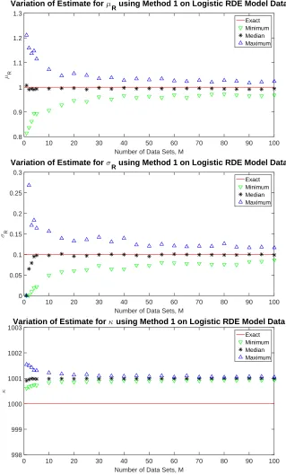
In Figure 3, the red line indicates the exact values of µR = 1, σR = 0.1 and κ = 1000. Using 100 different draws ofM data sets, we have plotted the largest, smallest and median estimated values for each parameter reflecting the extent which group of M has on the resulting estimate. We note that whenM is small (M <30), the range of possible estimates vary more than whenM is large, especially forµR andσR. However, even when using only 1 data set, the median estimate is quite accurate for bothµRandκ. In order to obtain close to the same level of accuracy for the median value ofσR, we needM ≥5 (also see Table 1). We do notice that the estimate forκ is always overestimated with a median value of approximately 1001; however, this only represents a 0.10% error in the estimated value. In fact, the maximum percent relative error in κdoes not vary much as a function of the number of data sets. We also observe that although we are assumingκis constant, we do have a small standard deviation of about 0.25 in the estimate ofκsimply due to the variation in the estimated value ofκgiven different data sets. However, Table 1 shows much more variation in the range of estimates for both µR and σR as a function of the number of data sets available. Ten or more data sets are required to obtain estimates with less than 10% relative error inµR; however, even with 100 data sets from the physical system, there is still the potential of having more than 15% relative in the estimate ofσR. Recall that the accuracy of the estimate depends onwhichM data sets are used in the estimation. Even though the potential is to have over 10% relative error usingM = 100 data sets; only 16% of the random draws of 100 data sets resulted in percent relative error more than 10%. IfM ≥ 70, then less than 25% of the time there is an estimate with a percent relative error of greater than 10% and when

M ≥ 25, then less than 40% of the time, there is an estimate for σR with more than 10% relative error. In summary, using Method 1 for estimating the parameters in the RDE logistic model, depending on the number of data sets available and which data sets are in this group, we were able to obtain good estimates for both κ and µR with as little as 1 data set. However, to ensure relative error less than 10% in µR, it was best to use 10 or more data sets if possible. The estimate forσR was much more difficult. Since σR is smaller with an exact value of only 0.10, it is much harder to estimate with the same degree of percent relative error. Nonetheless, with 15 or more data sets, we could obtain estimates within 0.05 of the actual value.

Note that even though the synthetic data was generated using the Logistic RDE model, this is identical to generating the data using the Bernoulli RDE model with β = 1. Therefore, the parameter estimation problem could be considered for the Bernoulli model in which we need to estimate not only µR, σR, and

κbut β as well. Therefore, we also attempted to estimate these parameters using only M = 15 data sets and obtained the results in Table 2. The estimates are comparable to those obtained when using the sample deterministic logistic model and estimating one less parameter.

We repeat the parameter estimation problem for the Logistic RDE model using the noisy synthetic data from the Logistic RDE Model (first plot in Figure 2). We only consider M = 15 in this trial. The results are given in Table 3 which are comparable to the results we saw using synthetic data without noise added. Adding the noise to the data did, however, result in a slightly larger standard deviation of 2.49 for κeven though κ is assumed constant. However, when noise is added to the data, it is expected that there will be some variation simply due to the variation in the estimates. We note, though, the calculated standard deviation inκis small compared to the magnitude ofκ.

(9)

-Number of Data Sets, M

0 10 20 30 40 50 60 70 80 90 100

µ R

0.8 0.9 1 1.1 1.2 1.3

Variation of Estimate for µ

R using Method 1 on Logistic RDE Model Data

Exact Minimum Median Maximum

Number of Data Sets, M

0 10 20 30 40 50 60 70 80 90 100

σ R

0 0.05 0.1 0.15 0.2 0.25 0.3

Variation of Estimate for σ

0 10 20 30 40 50 60 70 80 90 100

κ

998 999 1000 1001 1002

1003Variation of Estimate for

κ using Method 1 on Logistic RDE Model Data

(10)

Table 1: Variation of Percent Relative Error in Parameter Estimate for Logistic RDE Model using Synthetic Data with No Noise Added Using Method 1 with 100 Different Random Draws ofM Data Sets.

µR

M Max Perc. Rel. Error Med Perc. Rel. Error

1 21.13% 0.77%

2 16.35% 0.88%

3 13.78 % 0.67%

4 14.74% 0.91%

5 11.47% 0.65%

10 9.39% 0.54%

15 7.19% 0.44%

20 5.56% 0.32%

σR

M Max Perc. Rel. Error Med Perc. Rel. Error

1 100.00% 100.00%

2 168.57% 35.05%

3 90.27% 20.86%

4 83.46% 5.04%

5 77.92% 1.89%

10 56.25% 2.01%

15 42.55% 1.50%

20 40.04% 4.11%

40 39.81% 0.15%

60 21.25% 0.82%

80 26.42% 1.04%

100 16.75% 1.09%

Table 2: Parameter Estimates for Bernoulli RDE Model using Synthetic Logistic RDE Model Data with No Noise Added Using Method 1 with 100 Different Random Draws ofM = 15 Data Sets.

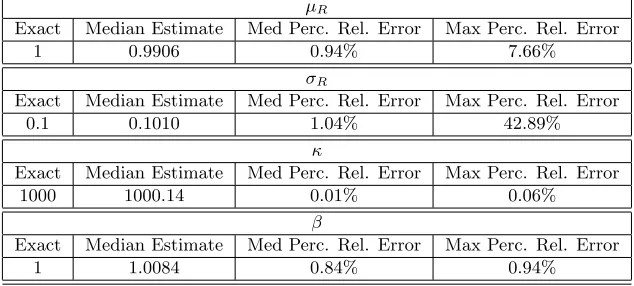
µR

Exact Median Estimate Med Perc. Rel. Error Max Perc. Rel. Error

1 0.9906 0.94% 7.66%

σR

0.1 0.1010 1.04% 42.89%

κ

1000 1000.14 0.01% 0.06%

β

(11)

Table 3: Parameter Estimates for Logistic RDE Model using Synthetic Data with Noise Added Using Method 1 with 100 Different Random Draws ofM = 15 Data Sets.

µR

1 0.9958 0.42% 7.49%

σR

0.1 0.0971 2.90% 47.46%

κ

1000 1000.17 0.02% 0.17%

Table 4: Parameter Estimates for Bernoulli RDE Model using Synthetic Data withβ= 1.5, No Noise Added, Using Method 1 with 100 Different Random Draws ofM = 15 Data Sets.

µR

1 0.9896 1.04% 8.09%

σR

0.1 0.0956 4.34% 51.52%

κ

1000 1000.03 0.003% 0.34%

β

1.5 1.5131 0.87% 20.81%

7. Using data without noise (Tables 4 and 6), we obtain estimates similar to those obtained using synthetic data from the Logistic model for µR, σR andκ; however, the maximum relative error in the estimates for

β are slightly worse than expected. Some of the difficulty in the estimation may lie in the identifiability of the parameters in the sample deterministic model sinceκandβ are found jointly in the denominator in the term (x(_κtβ))β. To address this issue, we let ˜κ=κ

β _{in the sample deterministic differential equation and seek}

an estimate ˆqforq= [µR, σR,κ, β˜ ] in the system

dx(t)

dt =rx(t)

1−(x(t)) β

˜

κ

(20)

where the estimate forκcan be calculated as ˆκ= ˆκ˜(1/βˆ)_.

We compare the estimation of r, κ, and β in the original sample deterministic system to the estimates obtained in the re-parameterized sample deterministic system for one of the data sets (with no noise added) in which the estimate for β is poor. Figure 4 shows the results in the parameter estimation. Using the re-parameterized deterministic model produced more accurate estimates for not onlyβbut all three parameters. The original estimates are given by ˆr = 0.95, ˆκ = 987.34 and ˆβ = 7.75. The estimates using the re-parameterized system are given by ˆr= 0.98, ˆκ= 1000.03 and ˆβ= 3.04.

(12)

Table 5: Parameter Estimates for Bernoulli RDE Model using Synthetic Data with β = 1.5, With Noise Added, Using Method 1 with 100 Different Random Draws ofM = 15 Data Sets.

µR

1 1.0048 0.48% 6.48%

σR

0.1 0.1001 0.06% 40.26%

κ

1000 999.98 0.02% 0.27%

β

1.5 1.5002 0.01% 18.83%

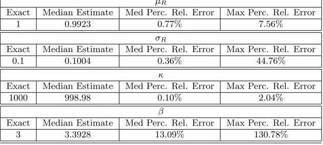
Table 6: Parameter Estimates for Bernoulli RDE Model using Synthetic Data withβ= 3, No Noise Added, Using Method 1 with 100 Different Random Draws ofM = 15 Data Sets.

µR

1 0.9923 0.77% 7.56%

σR

0.1 0.1004 0.36% 44.76%

κ

1000 998.98 0.10% 2.04%

β

3 3.3928 13.09% 130.78%

Table 7: Parameter Estimates for Bernoulli RDE Model using Synthetic Data with β = 3, With Noise Added, Using Method 1 with 100 Different Random Draws ofM = 15 Data Sets.

µR

1 1.0068 0.68% 6.96%

σR

0.1 0.0899 10.08% 44.72%

κ

1000 999.24 0.07% 1.33%

β

(13)

Time

0 1 2 3 4 5 6 7 8 9 10

Population

0 200 400 600 800 1000

1200

Model Fits Using Original Model and Reparameterized Bernoulli Models

Data

Fit with Original Model

Fit with Reparameterized Model

Parameter Estimates:

Original Model:

r = 0.95; κ = 987.34; β = 7.75

Reparameterized Model: r = 0.98; κ = 1000.03; β = 3.04

Figure 4: Comparison of the estimated values of r, κand β using synthetic Bernoulli model data (black stars) with β = 3 in the sample deterministic Bernoulli models given by Equation (19) (original model fit given by the solid blue line) and Equation 20 (reparameterized model fit given by the dashed blue line).

percent relative error of only 1.7% instead of 18.83% when using the original model. Similar improvement can be found when comparing Table 7 using the original sample deterministic system and Table 9 using the re-parameterized sample deterministic system when β = 3. Although the maximum relative error in β is still about 19%, there are only 9 trials out of the 100 which resulted in an error of over 10%.

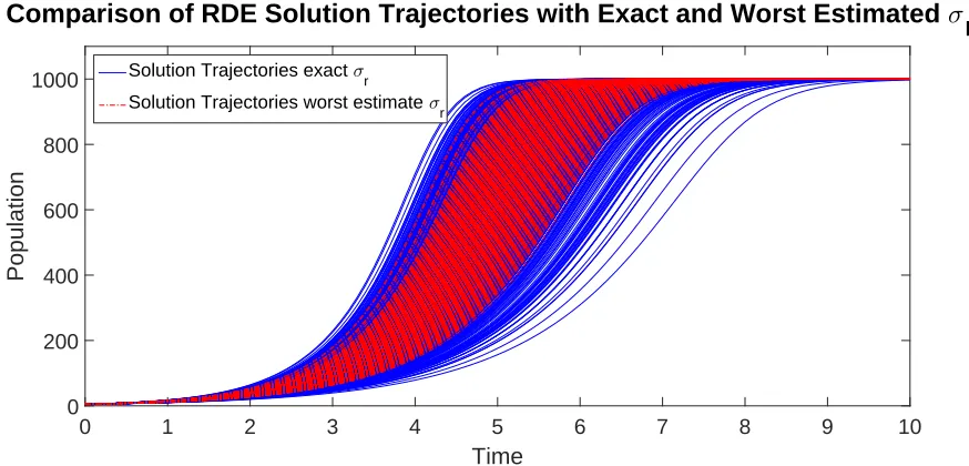
To summarize, using Method 1 to estimate parameters in a RDE model provided good estimates for both the mean of the random variable parameter and all constant parameters in the model in the examples presented for the Logistic RDE Model and the Bernoulli RDE Model with either β = 1.5 orβ = 3 when synthetic noisy data was used in the estimation problem. When usingM = 15 data sets, the accuracy ofσR depended onwhichdata sets were used in the estimation problem. Figure 5 shows the difference in the RDE solution or collection of solution trajectories to the sample deterministic equation when using the exact value of σR compared to the estimate which resulted in the worse percent relative error when using β = 3 and the re-parameterized sample deterministic system. In this case, σR was underestimated at approximately 0.06 (compared to the exact value of 0.1). We can see that the inaccuracy in the estimated value of σR resulted in less variability in the collection of solution trajectories. We expect this type of underestimation when the data sets used in the estimation problem are very similar with little variability in their growth rate. Nonetheless, the more data sets we are able to use, the more accurate we expect the estimate for

σR (see Table 1). We do note, however, that when implementing this method, one must still address the identifiability of parameters in the sample deterministic system. We found that a re-parameterization of the sample deterministic system provided much better estimates of the RDE parameters than when using the original system in which there was an issue with identifiability.

Using this method, we also tested the ability to estimate the random parameter R ifR had a Weibull distribution with scale parameter A = 1 and shape parameter B = 10, R ∼ W(A, B). As before, we generated 1000 different solution trajectories without noise, first plot in Figure 6, and with noise, second plot in Figure 6. We then estimated the parameters A and B of the Weibull statistical distribution for R

(14)

Table 8: Parameter Estimates for Bernoulli RDE Model using Synthetic Data with β = 1.5, With Noise Added, Using Method 1 with Reparameterized Sample Deterministic System and 100 Different Random Draws ofM = 15 Data Sets.

µR

1 0.9958 0.42% 7.45%

σR

0.1 0.0981 1.86% 49.24%

κ

1000 1000.07 0.008% 0.15%

β

1.5 1.5010 0.07% 1.70%

Table 9: Parameter Estimates for Bernoulli RDE Model using Synthetic Data withβ= 3, With Noise Added, Using Method 1 with Reparameterized Sample Deterministic System and 100 Different Random Draws of

M = 15 Data Sets.

µR

1 0.9986 0.14% 7.44%

σR

0.1 0.0949 5.08% 39.28%

κ

1000 999.82 0.02% 0.62%

β

(15)

Time

0 1 2 3 4 5 6 7 8 9 10

Population

0 200 400 600 800 1000

Comparison of RDE Solution Trajectories with Exact and Worst Estimated

σ

R

Solution Trajectories exact σ

r

Solution Trajectories worst estimate σ

r

Figure 5: Comparison of the RDE solution or collection of solution trajectories to the sample deterministic system for the RDE Model using the exact value for σR and the estimated value for σR, R ∼ N(µR, σR), whenβ= 3 and κ= 1000 in Bernoulli RDE model given by Equation (18).

Table 10: Parameter Estimates for Logistic RDE Model using Synthetic Data withR∼ W(1,10), No Noise Added, Using Method 1 with 100 Different Random Draws ofM = 15 Data Sets.

Scale ParameterA

1 0.9961 0.3881% 9.17%

Shape ParameterB

10 10.6128 6.13% 113.82%

κ

1000 999.99 0.0007% 0.003%

{rk}Mk=1 to estimate the statistical parametersA andB of the Weibull distribution. To do this, we use the

(16)

Time

0 1 2 3 4 5 6 7 8 9 10

Population

0 200 400 600 800 1000

Synthetic Logistic RDE Model Data Sets, R ~ W(1,10)

Time

0 1 2 3 4 5 6 7 8 9 10

Population

0 200 400 600 800 1000

Synthetic Logistic RDE Model Data Sets with Noise, R ~ W(1,10)

Figure 6: One thousand synthetic data sets without noise added (first plot) and with noise added (second plot) for the Logistic RDE Model (Eq. (3)) assumingR∼ W(1,10) andκ= 10000.

Table 11: Parameter Estimates for Logistic RDE Model using Synthetic Data withR∼ W(1,10), No Noise Added, Using Method 1 with 100 Different Random Draws ofM = 100 Data Sets.

Scale ParameterA

1 1.0010 0.10% 2.98%

Shape ParameterB

10 10.1268 1.27% 27.18%

κ

(17)

Table 12: Parameter Estimates for Logistic RDE Model using Synthetic Data with R ∼ W(1,10), With Noise Added, Using Method 1 with 100 Different Random Draws ofM = 15 Data Sets.

Scale ParameterA

1 0.9981 0.19% 7.25%

Shape ParameterB

10 10.1252 1.25% 82.11%

κ

1000 999.76 0.02% 0.44%

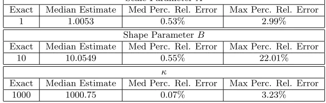
Table 13: Parameter Estimates for Logistic RDE Model using Synthetic Data with R ∼ W(1,10), With Noise Added, Using Method 1 with 100 Different Random Draws ofM = 100 Data Sets.

Scale ParameterA

1 1.0053 0.53% 2.99%

Shape ParameterB

10 10.0549 0.55% 22.01%

κ

(18)

5.2 Method 2 Results

In order to use Method 2, we must also first derive a pointwise equivalent SDE for each model and then approximate the SDE with an appropriate deterministic system. In order to use a pointwise equivalent SDE for model selection, the RDE model has to be in the form of either Equation (10) or (12). We first transform both the logistic RDE model and Bernoulli RDE model into the appropriate form and derive the pointwise equivalent SDE for each in Section 5.2.1 and 5.2.2 respectively.

5.2.1 Derivation of Pointwise Equivalent SDE for Logistic Model

The deterministic logistic growth model is given by

dx dt =rx

1−x

κ

.

We first transform the deterministic model by lettingy= 1

x. Then

dy

dt = −

1

x2

dx dt

= −1

x2

rx1−x

κ

= −r

₁

x−

1

κ

= −r

y− 1

κ

withy(0) = 1

x0

. The transformed RDE is then given by

dy(t;Q)

dt =−R

y(t;Q)− 1

κ

, y(0;Q) =y0

which has the form of Equation (12) withQ=R,%=−1,γ(t) = 0, andc=−1

κ. The pointwise equivalent

RDE inY(t) can be found using the form in Equation (13). Givenµ=µR and

˜

h(t) =σ2₀%0(t)

Z t

0

%0(s)ds=−σ2R

Z t

0

−1ds=σ_R2t,

the equivalent SDE is given by

dY(t) = −µR+σR2t

Y(t)−1

κ

dt+√2tσR

Y(t)−1

κ

dW(t), Y(0) =y0.

To determine the pointwise SDE in X(t), we letX(t) = 1

Y(t) and use Itˆo’s formula, the chain rule for Itˆo calculus ([2]), to finddX(t). Let

dY(t) =g(t, Y(t))dt+σ(t, Y(t))dW(t),

and assume his a function of t and y that is continuously differentiable int and twice differentiable in y. Then Itˆo’s formula gives the chain rule for differentiation as

dh(t, Y(t)) = ∂h(t, Y(t))

∂t dt+

∂h(t, Y(t))

∂x dY(t) +

1 2σ

2₍_{t, Y}₍_t₎₎∂2h(t, Y(t))

(19)

Applying this toX(t) = 1

Y(t), we have

dX(t) = − 1

Y2₍_t₎

−µR+σ2Rt

Y(t)−1

κ

dt+√2tσR

Y(t)−1

κ

dW(t)

+ 1

Y3₍_t₎

_√

2tσR

Y(t)−1

κ

2

dt

= 1

Y(t)

"

(µR−σ2Rt)

1− 1

κY(t)

+ 2tσ2

R

1− 1

κY(t)

2#

dt−√2tσR 1

Y(t)

1− 1

κY(t)

dW(t)

= X(t)

"

(µR−σ2Rt)

1−X(t)

κ

+ 2tσ2

R

1−X(t)

κ

2#

dt−√2tσRX(t)

1−X(t)

κ

dW(t)

Therefore, the pointwise equivalent SDE to the logistic RDE model given in Equation (3) is given by

dX(t) =X(t)

"

(µR−σR2t)

1−X(t)

κ

+ 2tσ2_R

1−X(t)

κ

2#

dt−√2tσRX(t)

1−X(t)

κ

dW(t), X(0) =X0.

We note that theSDE deterministic approximation is given by

dx dt =x

"

(µR−σ2Rt)

1−x(t)

κ

+ 2tσ2_R

1−x(t)

κ

2#

, x(0) =x0. (21)

Note, that the deterministic system contains all three parameters which must be estimated to fully define the RDE model,µR,σR, andκ.

5.2.2 Derivation of Pointwise Equivalent SDE for Bernoulli Model

In a similar manner, we can derive the pointwise equivalent RDE for the Bernoulli model. The deterministic Bernoulli model is given by

dx dt =rx

1−x

κ

β

.

We transform this deterministic model by lettingy= 1

xβ. Then

dy

dt = − β xβ+1

rx

1−x

κ

β

= −rβ

₁

xβ − 1

κβ

= −rβ

y− 1

κβ

withy(0) = 1

xβ₀. The transformed RDE is then given by

dy(t;Q)

dt =−Rβ

y(t;Q)− 1

κβ

, y(0;Q) =y0

which has the form of Equation (12) withQ=R,%=−β,γ(t) = 0, andc=− 1

κβ. The pointwise equivalent RDE inY(t) can be found using the form in Equation (13). Givenµ=µR and

˜

h(t) =σ₀2%0(t)

Z t

0

%0(s)ds=−βσR2

Z t

0

(20)

the pointwise equivalent SDE inY(t) is given by

dY(t) = −βµR+β2σR2t

Y(t)− 1

κβ

dt+√2tβσR

Y(t)− 1

κβ

dW(t), Y(0) =y0.

As in the previous section, we need to transform the SDE into an SDE in X(t). We let X(t) = 1

Y1/β₍_t₎. Then applying Itˆo’s formula we have

dX(t) = − 1

βY1/β+1₍_t₎

−βµR+β2σR2t

Y(t)− 1

κβ

dt+√2tβσR

Y(t)− 1

κβ

dW(t)

+ 1

βY1/β+2₍_t₎

1

β + 1

√ 2tβσR

Y(t)− 1

κβ

2

dt

= 1

Y1/β₍_t₎

"

(µR−βσR2t)

1− 1

κβ_Y₍_t₎

+ 2tσ2

R(1 +β)

1− 1

κβ_Y₍_t₎

2#

dt

− √

2tσR

Y1/β₍_t₎

1− 1

κβ_Y₍_t₎

dW(t)

= X(t)



(µR−βσR2t) 1−

_X₍_t₎

κ

β!

+ 2tσ2

R(1 +β) 1−

_X₍_t₎

κ

β!2  dt

−√2tσRX(t) 1−

_X₍_t₎

κ

β!

dW(t)

Therefore, the pointwise equivalent SDE to the Bernoulli RDE model given in Equation (18) is given by

dX(t) = X(t)



(µR−βσ2Rt) 1−

_X₍_t₎

κ

β!

+ 2tσ2

R(1 +β) 1−

_X₍_t₎

κ

β!2  dt

−√2tσRX(t) 1−

_X₍_t₎

κ

β!

dW(t), X(0) =X0.

We note that the deterministic approximation for this SDE is given by

dx dt =x

"

(µR−βσR2t)

1−x

κ

β

+ 2tσ_R2(1 +β)

1−x

κ

β2 #

, x(0) =x0 (22)

which again contains all the necessary parametersµR,σR,κandβ which must be estimated.

5.2.3 Results

We use the built-in Matlab programfminsearchto minimize the cost function given in Equation (16) where

fs(t,q) is the solution to the deterministic approximation for the pointwise equivalent SDE given by either Equation (21) or Equation (22), depending on the data set (synthetic data from the Logistic or Bernoulli RDE model, respectively). As done in testing the first method, the initial guess is set as 1.10q0whereq0 is

the exact value. We consider one random data set drawn from the 1000 possible synthetic data sets generated without noise (see Figure 1)) and estimateµR,σR,κ, andβ (for the Bernoulli model only). We do this 100 times. The estimated values are given in Tables 14, 15 and 16 for synthetic data from the Logistic model, Bernoulli model withβ= 1.5, and Bernoulli model withβ= 3 respectively.

(21)

Table 14: Parameter Estimates for Logistic RDE Model using Synthetic Data, With No Noise Added, Using Method 2 with 100 Different Random Draws ofOneData Set.

µR

1 0.9927 0.73% 22.81%

σR

0.1 2.95e-08 100% 100%

κ

1000 1000.98 0.10% 0.21%

relative error across 100 different individual data sets was approximately 23 - 26%. We also implement the parameter estimation problem using the re-parameterization ˜κ=κβ _{as above and also}_γ₌_βσ2

R where the

estimate forκcan be calculated as ˆκ= ˆ˜κ(1/βˆ)and the estimate forσR is calculated as ˆσR=

q

ˆ

γ/βˆ. Results in Table 17 and 18 indicate that the re-parameterization has little effect on the resulting estimates. We do note that there was one result when β = 3 which resulted in a relative error of about 12% in the estimate for β; however, this was one case in the 100 trials. The main problem in the estimation results are in the estimation ofσR. Similar to what we obtained using the first method, it was impossible to estimateσRusing only one data set. In the first method, σR was calculated to be 0 when only one data set was available; in this second method, σR is an estimated parameter in the deterministic approximation, but the estimation is still approximately 0. However, this is understandable, since there is no variance with only one data set. Therefore, we reformulate the cost function to incorporate multiple data sets and seek a realization

ˆ ˜

qNRDE2= arg min_q_∈_Ω

q

˜

JRDEN 2(q;z). (23)

of

˜ qN_RDE

2 = arg min_q_∈_Ω

q

˜

J_RDEN

2(q;Z)

where

˜

J_RDEN ₂(q;Z) = M

X

m=1

1

N

X

k=1

(Z_km−fs(tk;q))

2

!

(24)

withM the number of data sets {Zm}available.

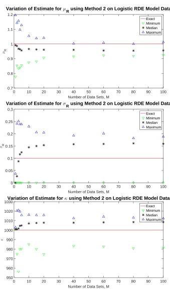
Figure 7 shows the results using synthetic data from the Logistic RDE model with no noise added when varying the number of data sets available and minimizing Equation (24). We note that the median estimate for µR and κare best when only one data set is used, and both approach a limiting value when M >20. The value forµRapproaches an underestimate with approximately 4-4.5% relative error, whileκapproaches an overestimate with approximately 0.8% relative error. We note that as M is increased, the maximum relative error in the estimate for µR is decreased as we also saw using the first method. For M ≥5, the maximum percent relative error in κis between about 1.5-2%. We see a different trend in the estimate for

σR, however. Even though the median estimate forσRalso approaches a limit, the minimum estimated value ofσR is 0 when considering 100 different random choices ofM data sets. The limiting value of the median is approximately 0.16 with about a 60% relative error. However, the estimated value of approximately 0 indicates that regardless of how many data sets are available, there is a potential to estimate that the random variableRis actually a constant. This result would indicate that the entire model should be a deterministic differential equation and not a random differential equation as assumed.

(22)

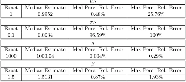
Table 15: Parameter Estimates for Bernoulli RDE Model withβ = 1.5 using Synthetic Data, With No Noise Added, and Method 2 with 100 Different Random Draws ofOneData Set.

µR

1 0.9952 0.48% 25.76%

σR

0.1 0.0034 96.59% 100%

κ

1000 1000.04 0.004% 0.29%

β

1.5 1.5131 0.87% 1.93%

Table 16: Parameter Estimates for Bernoulli RDE Model withβ= 3 using Synthetic Data, With No Noise Added, and Method 2 with 100 Different Random Draws ofOneData Set.

µR

1 0.9794 2.05% 26.01%

σR

0.1 0.0030 96.95% 100%

κ

1000 1000.04 0.004% 0.14%

β

3 3.0356 1.19% 3.16%

Table 17: Parameter Estimates for Bernoulli RDE Model with β = 1.5 using Synthetic Data and the reparameterization ˜κ=κβ _and_γ₌_βσ2

R, With No Noise Added, and Method 2 with 100 Different Random Draws ofOne Data Set.

µR

1 0.9872 1.28% 23.02%

σR

0.1 0.02 79.81% 100%

κ

1000 1000.02 0.002% 0.02%

β

(23)

0 10 20 30 40 50 60 70 80 90 100

µ R

0.7 0.8 0.9 1 1.1 1.2

Variation of Estimate for µ

0 10 20 30 40 50 60 70 80 90 100

σR

0 0.05 0.1 0.15 0.2 0.25 0.3

Variation of Estimate for σ

0 10 20 30 40 50 60 70 80 90 100

κ

950 960 970 980 990 1000 1010 1020

1030Variation of Estimate for

κ using Method 2 on Logistic RDE Model Data

(24)

Table 18: Parameter Estimates for Bernoulli RDE Model withβ= 3 using Synthetic Data and the reparam-eterization ˜κ=κβ _and_γ ₌_βσ2

R, With No Noise Added, and Method 2 with 100 Different Random Draws ofOne Data Set.

µR

1 0.9979 0.21% 26.01%

σR

0.1 0.0127 87.31% 100%

κ

1000 1000.03 0.003% 0.31%

β

3 3.0384 1.28% 11.73%

(25)

6 Parameter Estimation with Experimental Data using Method 1

In this section, we use method 1 for estimating the parameters in a RDE logistic and RDE Bernoulli growth model using longitudinal data collected from algae growth. In a paper by Banks et. al. [3], longitudinal data was collected from four replicate population experiments with green algae, formally known asRaphidocelis subcapitata. Four beakers were initially seeded with 1L of Bold’s Basal Media (BBM) and then conditions were set to maintain a chemostat steady-state equilibrium system, constant volume, sufficient oxygen supply, and homogeneous state; details on the experimental collection process can be found in [3]. Two measurements for each of the four replicates were taken twice a day at 9 am and 5 pm daily; the data is shown in Figure 8. Two measurements were taken from each beaker initially so the data could be averaged to minimize human measurement error; however, we consider each data set as an individual data set regardless of whether the data came from the same beaker or a different beaker.

Time (hours)

0 50 100 150 200 250 300 350 400 450

Cell Count

0 1000 2000 3000 4000 5000

6000 Longitudinal Data for Green Algae (Raphidocelis subcapitata)

Population 1a Population 1b Population 2a Population 2b Population 3a Population 3b Population 4a Population 4b

Figure 8: This figure shows the longitudinal data for the two measurements of each of the four replicates of Raphidocelis subcapitata.

We first assume the data satisfies the logistic RDE growth model with normally distributed random variable parameters for the growth rateR∼ N(µR, σR) and limiting capacityK∼ N(µK, σK). In addition, we assume, as done in the paper by Banks et. al. [3], that the initial population is also an unknown parameter which must be estimated; in this case, we assume it is a random variable parameter, X0 ∼ N(µX0, σX0).

We note that we initially assume all parameters are random variable parameters; however, for a parameter

Q, if the estimated value ofσQ is small relative to the valueµQ, we can instead declare this parameter a constant parameter in the model. To estimate the individual data parameters for the sample deterministic system required in method 1, we use an initial guess ofr= 0.02,κ= 4100, andx0= 414. The estimates for

the eight individual data sets are given in Table 19. We notice the variability in both the estimates across the four beakers but also the variation in estimates even using data from the same beaker.

Table 19: Parameter Estimates in the Logistic Sample Deterministic Model for Individual Algae Data Sets.

Data Set r κ x0

1a 0.0187 4611.42 399.17 1b 0.0179 4398.34 430.31 2a 0.0189 4281.04 320.84 2b 0.0171 4322.88 360.53 3a 0.0174 4348.04 358.31 3b 0.0184 4210.42 291.76 4a 0.0192 3988.83 248.42 4b 0.0180 4262.62 308.07

(26)

thenumber of data sets and which data sets were used affect the estimated values for both the mean and standard deviation of each random variable parameter. Since we only have eight total data sets, we consider each combination ofM data sets, M = 2, ...,8 in the calculation of µQ (Equation (8)) and σQ (Equation (9)) for each parameter Q. The results are shown in Figure 9. As expected, there is a larger spread in possible estimates when only a few data sets are used; however the median estimate is fairly constant across

M. The estimated values for all statistical parameters when using all eight data sets are given in Table 20. Figure 10 illustrates the RDE model solution together with the data under the assumptions that different model parameters are random variable parameters or constant parameters. We note that σR ≈ 0.04µR,

σK ≈0.04µK and σX0 ≈0.17µX0. The RDE solution or collection of solutions trajectories to the sample

deterministic equation appears to ‘cover’ the data best when all model variables are assumed to be random model parameters (first plot) or when the limiting capacityK and initial cell countX0are assumed random

(second row, second column plot). This comparison between the data and model simulations is similar to what is illustrated in Figure 5 with synthetic data when the value ofσRwas underestimated. However, if the noise level E is increased to approximately 10% of the limiting capacity, the model simulations with noise added encompasses the data near the limiting capacity however is too large for the initial cell count and can cause negative or zero cell count at the lower cell count population; see Figure 11. Therefore, it may be more appropriate to assume a nonconstant variance statistical model.

M

1 2 3 4 5 6 7 8 9

Estimated µR 0.016 0.0165 0.017 0.0175 0.018 0.0185 0.019 0.0195 0.02

Estimated µ

R Depending on Combination of M Data Sets

M

1 2 3 4 5 6 7 8 9

Estimated

σR

×10-3

0 0.5 1 1.5

Estimated σ

M

1 2 3 4 5 6 7 8 9

Estimated µK 4000 4100 4200 4300 4400 4500 4600

Estimated µ

K Depending on Combination of M Data Sets

M

1 2 3 4 5 6 7 8 9

Estimated σK 0 50 100 150 200 250 300 350 400 450

Estimated σ

M

1 2 3 4 5 6 7 8 9

Estimated µx0 250 300 350 400 450

Estimated µ

x0 Depending on Combination of M Data Sets

M

1 2 3 4 5 6 7 8 9

Estimated σx0 0 20 40 60 80 100 120 140

Estimated σ

(27)

Figure 10: Each plot shows 1000 simulations of the logistic RDE model(dark grey) with the data (black) and with constant variance noise E ∼ N(0,1002_{) (light grey). The first plots assumes} _R _{∼ N}₍_µ

R, σR),

K∼ N(µK, σK), andX0∼ N(µX0, σX0) with estimated values given in Table 20. The second plot assumes

bothRandKare random variable model parameters butx0is a constant parameter. The third plot assumes

bothRandX0are random variable model parameters butκis constant. The fourth plot assumes bothKand

X0 are random variable model parameters butris constant. The fifth plot shows the simulations assuming

onlyR is a random variable model parameter. The sixth plot shows the simulations if onlyK is a random variable parameter. The seventh plot shows the simulations if only X0 is a random variable parameter.

(28)

Table 20: Statistical Parameter Estimates for Random Variable Model Parameters in the Logistic RDE Model using Eight Algae Cell Count Data Sets.

Parameter Estimate

µR 1.82·10−2

σR 7.38·10−4

µK 4302.95

σK 175.67

µX0 339.68

σX0 59.18

Figure 11: This plot shows 1000 simulations of the logistic RDE model(dark grey) with the data (black) and with increased constant variance noise E ∼ N(0,4002_{) (light grey) with random variable parameters}

R∼ N(µR, σR),K∼ N(µK, σK), andX0∼ N(µX0, σX0).

In fact, in the paper by Banks et. al. [3], they demonstrated that the algae data exhibited proportional noise, or nonconstant variance noise, of the form

Zj =h(tj;q0) +hγ(tj;q0)Ej, Var(Zj) =σ20h 2γ₍_t

j;q0) (25)

where the best choice forγ was shown to be γ= 1. This is different from the assumptions made when we formulated method 1 above. We had initially made the assumption that the statistical model had constant variance noise, i.e.,

Zj =h(tj;q0) +Ej, Var(Zj) =σ20.

To incorporate the nonconstant variance, for each individual data set, we seek a generalized least squares estimate

qN_GLS= arg min

q∈Ωq

J_GLSN (q;Z)

with realization

ˆ

qN_GLS = arg min

q∈Ωq

J_GLSN (q;z)

where the cost functionJN

GLS is defined by

J_GLSN (q;Z) = 1

N

X

k=1

wk(Zk−f(tk;q))

2

(26)

(29)

Table 21: Parameter Estimates in the Logistic Sample Deterministic Model for Individual Algae Data Sets When MinimizingJN

GLS (Eq. (26)).

Data Set r κ x0

1a 0.0266 4394.85 224.49 1b 0.0253 4224.49 258.68 2a 0.0245 4237.32 209.42 2b 0.0211 4177.31 271.39 3a 0.0222 4217.35 257.20 3b 0.0238 4104.45 200.28 4a 0.0214 3957.20 243.74 4b 0.0248 4124.85 185.06

Table 22: Statistical Parameter Estimates for Random Variable Model Parameters in the Logistic RDE Model using Eight Algae Cell Count Data Sets when Assuming Nonconstant Variance in the Statistical Model (i.e., when minimizingJN

GLS).

Parameter Estimate

µR 2.37·10−2

σR 1.97·10−3

µK 4179.73

σK 126.05

µX0 231.28

σX0 31.18

in the same way as before and obtain similar trends in the results as in the ordinary least squares method. The estimated values when using all eight data sets is given in Table 22. Figure 12 illustrates the RDE model solution with noise added using the estimated random variable parameters defined by the statistical parameters given in Table 22. We note that the RDE solution is similar to the one found when assuming constant variance; however, there appears to be a slightly better estimate ofX0, a smaller relative variance

in the limiting capacity,σ_K2, and a larger relative variance in the growth parameterσ_R2.

We also fit the RDE Bernoulli growth model assuming nonconstant variance in the data (i.e., the statistical model is given by Equation (25)). We minimizeJ_GLSN in Equation (26) for the sample deterministic Bernoulli model for each data set and obtain the estimates in Table 23. Comparing parameter estimates for the logistic sample deterministic system in Table 21 and for the Bernoulli sample deterministic system in Table 23, we note that the estimates in the Bernoulli model forrandκare smaller than those in the logistic model while the initial data x0 is larger in the Bernoulli model. Moreover, β is estimated to be slightly larger than 1

where β = 1 indicates the logistic model. Using these estimates with Equations (8) and (9), we obtain the estimates for the statistical parameters given in Table 24 when using all eight data sets. The trend when using a subset of M data sets is shown in Figure 13. In these results, we note that σR ≈0.08µR,

σK ≈0.03µK, σX0 ≈0.13µX0 andσβ≈0.006µβ. Therefore, the relative value ofσβ is only approximately

0.6% the value ofµβ, and hence, we assumeβ is a constant parameter in the Bernoulli RDE growth model. The plot in Figure 14 shows 1000 simulations of the Bernoulli RDE growth model assuming random variable parameters R,K and X0 with a constant parameterβ. We also include the model with 10% relative noise

(30)

Figure 12: Each plot shows 1000 simulations of the logistic RDE model(dark grey) with the data (black) and with 2.5% relative noise or nonconstant variance noise (first plot) and 10% relative noise (second plot). In both plots, we assume R∼ N(µR, σR), K ∼ N(µK, σK), andX0∼ N(µX0, σX0) with estimated values

given in Table 22.

Table 23: Parameter Estimates in the Bernoulli Sample Deterministic Model for Individual Algae Data Sets When MinimizingJN

GLS (Eq. (26)).

Data Set r κ β x0

1a 0.0247 4386.71 1.1553 236.56 1b 0.0232 4215.55 1.1721 273.21 2a 0.0228 4222.27 1.1642 219.26 2b 0.0195 4158.98 1.1647 282.61 3a 0.0205 4206.92 1.1536 269.69 3b 0.0221 4088.01 1.1691 209.64 4a 0.0198 3946.38 1.1538 255.36 4b 0.0231 4108.87 1.1664 193.61

Table 24: Statistical Parameter Estimates for Random Variable Model Parameters in the Bernoulli RDE Model using Eight Algae Cell Count Data Sets when Assuming Nonconstant Variance in the Statistical Model.

Parameter Estimate

µR 2.20·10−2

σR 1.84·10−3

µK 4166.71

σK 127.41

µβ 1.1624

σβ 7.20·10−3

µX0 242.49

(31)

M

1 2 3 4 5 6 7 8 9

Estimated µR 0.019 0.02 0.021 0.022 0.023 0.024 0.025

Estimated µ

M

1 2 3 4 5 6 7 8 9

Estimated

σR

×10-3

0 0.5 1 1.5 2 2.5 3 3.5 4

Estimated σ

M

1 2 3 4 5 6 7 8 9

Estimated µK 4000 4050 4100 4150 4200 4250 4300 4350

Estimated µ

M

1 2 3 4 5 6 7 8 9

Estimated σK 0 50 100 150 200 250 300 350

Estimated σ

M

1 2 3 4 5 6 7 8 9

Estimated µβ 1.15 1.155 1.16 1.165 1.17 1.175 Estimated µ

β Depending on Combination of M Data Sets

M

1 2 3 4 5 6 7 8 9

Estimated σβ 0 0.002 0.004 0.006 0.008 0.01 0.012 0.014

Estimated σ

β Depending on Combination of M Data Sets

M

1 2 3 4 5 6 7 8 9

Estimated µx0 200 220 240 260 280

Estimated µ

M

1 2 3 4 5 6 7 8 9

Estimated σx0 0 10 20 30 40 50 60 70

Estimated σ

(32)

Figure 14: This plot shows 1000 simulations of the Bernoulli RDE model(dark grey) with the data (black) and with 10% relative noise or nonconstant variance noise under the assumption that R ∼ N(µR, σR),

K∼ N(µK, σK),X0∼ N(µX0, σX0) andβ =µβ with estimated values given in Table 24.

7 Conclusions

In this paper, we investigated two methods for parameter estimation in a RDE model. The first method was based on approximating the RDE with its sample deterministic equation while the second method was based on first deriving the pointwise equivalent SDE model for the RDE model and then approximating the SDE model with a deterministic model. In both parameter estimation techniques, deterministic parameter estimation techniques were used once the appropriate deterministic system was identified.

In the first method, constant parameters for the deterministic system are estimated. These constants are then used to estimate the statistical parameters for the random variable distributions. We tested this method on two nested RDE models in which there was one random variable parameter. Depending on the number of data sets available, some of the statistical parameters were harder to estimate than others. We tested the method assuming either a normally distributed random variable parameter or a random variable parameter with a 2-parameter Weibull distribution. When testing the method with a normally distributed random variable parameter, depending on the random choice of data sets and how many data sets were used in the estimation, it could be difficult to obtain an extremely accurate estimate for the standard deviation. However, this makes intuitive sense since if the data sets behave similarly, then the variance (and hence the standard deviation) may be estimated smaller than the actual standard deviation. Figure 5 gives an illustration of the collection of solution trajectories if the standard deviation is estimated smaller than the actual standard deviation. When estimating the random variable parameter assumed to have a Weibull distribution, the shape parameter B was slightly more difficult to estimate; however, even though there is the potential for a poor estimate, in most cases, the relative error in both statistical parameters was less than 10% whenM = 15 orM = 100. In summary, the first parameter estimation technique was a viable method for the models analyzed in this paper.

(33)

viable method for the example models presented in this paper.

Finally, we applied the first method in estimating the random variable model parameters in both the logistic and Bernoulli RDE models using experimental data from algae growth. The resulting RDE solution using the random variable parameter estimates obtained from method 1 appear plausible when compared to the eight data sets. We also illustrated the differences in the RDE solution assuming one or multiple random variable parameters in the model and compared each scenario with the eight data sets. Visually, the RDE solution in which all model parameters were assumed to be random variables appears to be the best model for the data; however, unless the noise has a large enough variance, the resulting model with noise did not encompass the entire range in the cell count data. If we assumed a statistical model with constant variance, when the constant variance was large enough to encompass the large cell count, it was too large for the smaller cell count. Therefore, we reformulated method 1 to incorporate a nonconstant variance. We illustrated the slight differences in the estimated values and resulting solution curve with noise. In this case, assuming a 10% relative noise in the model simulation resulted in simulations which covered the range in the data while accounting for the size of the cell count. Furthermore, we approximated the random variable model parameters in the Bernoulli RDE model as well using the experimental data under the assumption of nonconstant variance in the statistical model. Similar results were found as with the logistic model. In general, we have shown that method 1 was a viable approach for estimating parameters in a random differential equation model not only using synthetic data but with experimental data as well.

Acknowledgements

This research was supported in part by the National Institute on Alcohol Abuse and Alcoholism under grant number 1R01AA022714-01A1, and in part by the Air Force Office of Scientific Research under grant number AFOSR FA9550-15-1-0298.

References

[1] Linda Allen. An Introduction to Stochastic Processes with Applications to Biology. Taylor and Francis Group, LLC, 2011.

[2] H. T. Banks, Shuhua Hu, and W. Clayton Thompson. Modeling and Inverse Problems in the Presence of Uncertainty. CRC Press, 2014.

[3] H.T. Banks, Elizabeth Collins, Kevin Flores, Prayag Pershad, Michael Stemkovski, and Lyric Stephen-son. Standard and proportional error model comparison for logistic growth of green algae (Raphidocelis subcapiala). Applied Mathematical Letters, 64:213–222, 2017.

[4] H.T. Banks and S. Hu. Nonlinear stochastic Markov processes and modeling uncertainty in populations. Mathematical Biosciences and Engineering, 9(1):1–25, 2012.

[5] H.T. Banks and Michele L. Joyner. Determinisitc methodology for comparison of nested stochastic models. CRSC-TR16-13, NCSU, Raleigh, NC, November, 2016.

[6] Stewart N. Ethier and Thomas G. Kurtz. Markov Processes: Characterization and Convergence, volume 282. John Wiley & Sons, 2009.

[7] Avner Friedman. Stochastic Differential Equations and Applications. Dover Publications, 2006.

[8] Thomas C. Gard. Introduction to Stochastic Differential Equations. Marcel Dekker, 1988.

(34)

[10] Thomas G. Kurtz. Solutions of ordinary differential equations as limits of pure jump Markov processes. Journal of Applied Probability, 7(1):49–58, 1970.

[11] Zeev Schuss. Theory and Applications of Stochastic Processes: An Analytical Approach, volume 170. Springer Science & Business Media, 2009.

[12] Tsu T. Soong. Random Differential Equations in Science and Engineering. Elsevier, 1973.

[13] Howard M. Taylor and Samuel Karlin. An Introduction to Stochastic Modeling. Academic Press, 2014.