Novel maximum likelihood approach for passive detection and localisation of multiple emitters

(1)

R E S E A R C H

Open Access

Novel maximum likelihood approach for

passive detection and localisation of multiple

emitters

Marcel Hernandez

Abstract

In this paper, a novel target acquisition and localisation algorithm (TALA) is introduced that offers a capability for detecting and localising multiple targets using the intermittent “signals-of-opportunity” (e.g. acoustic impulses or radio frequency transmissions) they generate. The TALA is a batch estimator that addresses the complex

multi-sensor/multi-target data association problem in order to estimate the locations of an unknown number of targets. The TALA is unique in that it does not require measurements to be of a specific type, and can be implemented for systems composed of either homogeneous or heterogeneous sensors. The performance of the TALA is

demonstrated in simulated scenarios with a network of 20 sensors and up to 10 targets. The sensors generate angle-of-arrival (AOA), time-of-arrival (TOA), or hybrid AOA/TOA measurements. It is shown that the TALA is able to successfully detect 83–99% of the targets, with a negligible number of false targets declared. Furthermore, the localisation errors of the TALA are typically within 10% of the errors generated by a “genie” algorithm that is given the correct measurement-to-target associations. The TALA also performs well in comparison with an optimistic

Cramér-Rao lower bound, with typical differences in performance of 10–20%, and differences in performance of 40–50% in the most difficult scenarios considered. The computational expense of the TALA is also controllable, which allows the TALA to maintain computational feasibility even in the most challenging scenarios considered. This allows the approach to be implemented in time-critical scenarios, such as in the localisation of artillery firing events. It is concluded that the TALA provides a powerful situational awareness aid for passive surveillance operations.

Keywords: Passive detection and localisation, Multi-sensor/multi-target data association, Maximum likelihood estimation, Gauss-Newton gradient descent, Cramér-Rao lower bound, Time-of-arrival measurements

1 Introduction

Recently, there has been great interest in the detection, localisation and tracking of noncooperative targets using passive sensors that exploit the “signals-of-opportunity” generated by such targets (e.g. see [1] and references therein). Typical applications include detection and local-isation of weapon firing events [2, 3] and locallocal-isation in wireless communication systems [4, 5], non-line-of-sight (e.g. urban) environments [6], and in search/rescue operations [7].

Passive surveillance has the advantage of covertness, and passive sensors are typically smaller, cheaper, and lower power than their active counterparts. This allows

Correspondence: [email protected]

Hernandez Technical Solutions Ltd, 38A Lower Chase Road, Malvern, Worcestershire WR14 2BZ, United Kingdom

passive sensors to be utilised in scenarios that would preclude the deployment of active sensors (e.g. such as in remote operations). Passive measurement exploitation has a long history, beginning with angle-of-arrival (AOA) emitter localisation [8]. Other commonly used passive measurements include time-of-arrival (TOA), time differ-ence of arrival (TDOA), frequency of arrival (FOA), and combinations thereof (e.g. again, see [1] and references therein).

Due to the intermittent nature of target signals in passive surveillance operations (e.g. artillery firings may occur in short bursts only every few days), recursive esti-mation techniques (e.g. such as the extended Kalman filter [9]) may be ineffective, because the interval between signals is too large to allow persistent target tracking. Therefore, it is common to perform batch estimation in

(2)

order to detect and localise target emitters, exploiting all measurements generated by the sensors within a time window, e.g. [2, 4, 5, 10–13]. The time window must be sufficiently large to account for target signal propagation delays between the sensors.

Previous work on passive emitter geo-location has largely concentrated on the case of a single target, thereby avoiding the problem of associating measurements to tar-gets. For example, maximum likelihood (ML) approaches have been developed for single target localisation using either TOA measurements [14], range measurements gen-erated by a multi-static passive radar [15], or TDOA measurements [16]. Target localisation using hybrid mea-surements has also been performed, with least squares (e.g. [4, 5]) and ML (e.g. [11, 12]) approaches devel-oped in order to localise a single emitter using hybrid AOA/TDOA measurements.

To-date, only a small number of papers have con-sidered the problem of localising multiple emitters [2, 10, 13, 17–20]. Some of these papers have addressed simplified scenarios with either perfect measurements [17, 18] or a known number of emitters [13]. The remain-ing papers have developed techniques specifically for a TOA measurement model [2, 10, 19, 20], and these approaches cannot be easily modified to deal with other measurement models (e.g. hybrid AOA/TOA measure-ments). Furthermore, as noted in [10], there remains a requirement to generalise existing approaches in order that they can exploit measurements generated by a net-work of heterogeneous sensors.

The target acquisition and localisation algorithm (TALA) introduced herein addresses the complex multi-sensor/multi-target data association problem, in order to detect and localise an unknown number of target sig-nals/events (e.g. such as acoustic impulses generated by artillery firings or intermittent radio frequency transmis-sions). The TALA is a batch estimator, and its novelty lies in the mechanism by which it circumnavigates the need to perform global multi-sensor/multi-target data associa-tion, e.g. as necessary in [20], thereby allowing the TALA to maintain computational feasibility, even for large-scale problems. Furthermore, unlike existing approaches (e.g. [2, 10, 19, 20]), the TALA does not require measure-ments to be of a specific type (i.e. TOA measuremeasure-ments) and can be implemented for systems composed of either homogeneous or heterogeneous sensors.

Specifically, the TALA initially performs nearest neigh-bour data association (e.g. see [21]) on a measurement-by-measurement basis, allowing each measurement to be associated with multiple hypothesised target locations. The algorithm formulates a set of potential target location hypotheses, and then performs Gauss-Newton (G-N) gra-dient descent (e.g. [24]) to provide maximum likelihood estimates of these locations, before a final downselection

step, ensures that each measurement is associated with no greater than one estimate.

This mechanism for handling the complex multi-sensor/multi-target association problem, based on manip-ulating multiple competing hypotheses, removes the need to perform global data association (which can be a com-putationally prohibitive combinatorial optimisation, e.g. see [22]), and is analogous to the track-oriented multiple hypothesis tracking (TOMHT) methodology introduced in [22]. However, unlike the TOMHT, the TALA is a non-recursive (i.e. “one-shot”) approach, rather than the update of an existing target set.

The remainder of this paper is organised as follows. In Section 2, the TALA is described. In Section 3, details are provided of the two measures of optimal estimation performance that are used to baseline the performance of the TALA. The first measure is the Cramér-Rao lower bound [23], and the second is a “genie” TALA that is given the correct measurement-to-target associations. In Section 4, simulation results are presented for scenar-ios in which all sensors provide hybrid AOA/TOA mea-surements, and scenarios in which 50% of the sensors provide only AOA measurements, with the remaining sensors providing only TOA measurements. A discus-sion is presented in Section 5 with concludiscus-sions following in Section 7. Section 6 provides details of recommen-dations for future work. Finally, Appendix A provides details of the methodology for determining initial can-didate target locations using the AOA and distance dif-ference of arrival (DDOA) measurements available in the simulations.

2 Target acquisition and localisation algorithm

2.1 Overview

The TALA is a batch estimation algorithm that utilises all measurements generated within a time window by an array of sensors, in order to detect and localise an unknown number of target events (i.e. intermittent sig-nals, such as acoustic impulses or radio frequency trans-missions). Initially, the TALA generates “candidate” target locations, and then performs “soft” nearest neighbour data association (e.g. [21]), allowing each measurement to be associated with more than one candidate location. This approach removes the need to perform global multi-sensor/multi-target data association, e.g. as necessary in [20], thereby maintaining computational feasibility, even for large scale problems.

(3)

potential divergence, line search and randomisation are used to ensure that each iteration increases the value of the likelihood. It is noted that alternative techniques, such as the Newton-Raphson (N-R) approach (e.g. [25]) or the Levenberg-Marquardt algorithm [26, 27], could also be used to perform the gradient descent and may offer similar performance.

2.2 Summary of the main steps

The main steps in the TALA are as follows:

1. Step 1: Determine initial candidate locations

• If possible (generally only in two-dimensional emitter geo-location), determine the

intersection between measurements generated by each pair of sensors.

• More generally, determine a candidate location that minimises a Mahalanobis-based distance metric using measurements generated by each pair of sensors.

• These points form the initial candidate (target) location set.

• In cases for which performing measurement intersection or Mahalanobis distance

minimisation is problematic/impossible, initial candidate locations should be randomly sampled within the surveillance region.

2. Step 2: Associate measurements and determine likelihood for each candidate location

• Determine the measurement from each sensor that has the greatest individual likelihood (or equivalently the smallest Mahalanobis distance) for each candidate location.

• This measurement is associated with the location provided that the individual likelihood is greater than a pre-specified threshold value.

• Each measurement is allowed to be associated with more than one candidate location.

• The overall likelihood of each candidate location is calculated using all of the associated measurements.

3. Step 3: Candidate location deletion

• The number of candidate locations can be large.

• To reduce the computational expense of the algorithm, at this stage, some of the candidate locations are deleted.

• A candidate location is deleted if it either has too few measurements associated with it or if it shares identical associations with another candidate target location that has a greater overall likelihood.

• Optionally, the candidate location is deleted if it shares any associations with another candidate target location that has a greater overall likelihood.

4. Step 4: Maximum likelihood estimation

• Using the candidate locations retained from Step 3, plus the measurements associated with each location, determine ML estimates via an iterative G-N approach.

• Optionally, measurement reassociation may be performed on each iteration of the G-N algorithm.

5. Step 5: Final downselection/outputs

• Perform downselection to ensure that each measurement is associated with only one ML estimate.

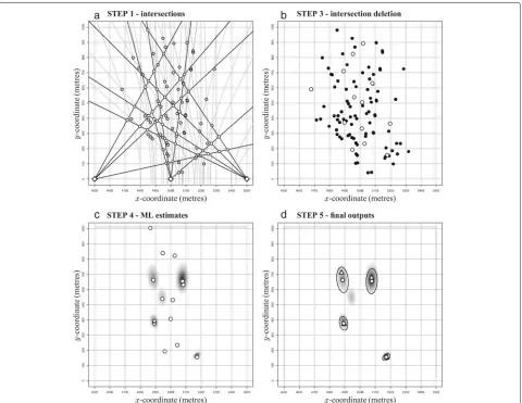
An illustrative example of the TALA is shown in Figs. 1 and 2.

2.3 Step 1: Determine initial candidate locations

An N sensor system is considered. Letn(i) denote the number of measurements, each of dimensionalitydi, gen-erated by sensori. Letz(i,j)denote thej-th measurement generated by sensori. It is assumed that target-generated measurements are corrupted by additive Gaussian noise1. Hence, for a target located at coordinatesX ∈ R3, each target-generated measurement at sensoriis given as fol-lows: error covariance of each target-generated measurement at sensori.

The first step in the TALA is to generate a set of ini-tial candidate location hypotheses, with these hypotheses then manipulated in order to determine ML estimates of the locations of an unknown number of targets. Therefore, it would seem prudent to choose candidate locations that are consistent with the measurements. To this end, the fol-lowing methodology is used to generate initial candidate locations:

(4)

Fig. 1An exemplar scenario with four target events and three sensors that provide hybrid AOA/TOA measurements. Shown are target events (marked bytriangles) and the sensors (marked bydiamonds); along with AOA measurements (black lines) and DDOA measurement hyperbolae (grey lines). Also shown is the likelihood map, withdark regionsshowing a normalised overall measurement likelihood close to unity, andwhite regions showing a normalised overall measurement likelihood close to zero. It is noted that this likelihood map is not calculated by the TALA and is shown for illustrative purposes only

point exists). In later simulations, the intersections between pairs of AOA measurements and pairs of DDOA measurements are used to generate initial candidate locations.

2. For more complex applications in which

measurement intersection cannot be performed (e.g. three-dimensional target geo-location, in which case the measurements are extremely unlikely to intersect because of the presence of measurement errors), for each pair of measurementszˆz(i1, .)z(i2, .)

, for i1=i2; a candidate locationXccan be determined by

minimising the Mahalanobis distance betweenzˆand

ˆ

f(X)f(X;i1)f(X;i2)

, i.e.

Xc = arg min X∈R3

(X)ˆ−1(X) (2)

where(X)(zˆ−fˆ(X)); andˆ is the error covariance of the measurementz.ˆ

It may be necessary to limit the number of can-didate locations by not considering all combinations

of sensor measurements in determining the intersec-tions (in two-dimensional applicaintersec-tions) or minimising (2) (in dimensional applications). Moreover, in three-dimensional geo-location applications, the optimisation in Eq. (2) may not be straightforward, and it may be more efficient to randomly select candidate locations within the surveillance region.

2.4 Step 2: Associate measurements and determine likelihood for each candidate location

It is assumed that for each sensor, a maximum of one mea-surement is generated by each target in the time window under consideration. Furthermore, for each candidate tar-get locationX, and each sensori:

1. The indexa(X;i)∈ {1,. . .,n(i)}of the measurement that is associated is the one with the largest

individual likelihood, i.e. nearest neighbour data association is performed (e.g. see [21]).

2. If every measurement generated by a sensor has an individual likelihood that is less than 100ξ% of the maximum valueli(max), then no measurement from

(5)

Fig. 2Demonstration of the TALA for the scenario with four targets.aStep 1: intersection of each pair of AOA measurements (white circles) and each pair of DDOA measurement hyperbolae (grey circles).bStep 3: intersections that are retained (white circles), and intersections that are deleted (black circles; deletion criterion 3 is not used).cStep 4: ML estimates.dStep 5: downselected ML estimates (circles), and the true target locations (triangles). Each ellipse shows the 5 standard deviation error covariance associated with each ML estimate

thresholdξ ∈[ 0, 1]is pre-specified3. It is noted that this approach is equivalent to gating the

measurement Mahalanobis distance with a threshold g=√−2 lnξ.

Therefore,a(X;i)is given as follows:

a(X;i) ⎧ ⎪ ⎨ ⎪ ⎩

arg max

j=1,...,n(i)li(X;j) ifj=max1,...,n(i)li(X;j)≥ξ×li(max)

−1 otherwise

(3)

whereli(X;j)denotes the individual likelihood at sensori as a result of associating thej-th measurementz(i,j)with candidate target locationX. For the measurement model

(1), this individual likelihood is given as follows:

li(X;j)=

1

(2π)di/2_det(_i)1/2exp

−1

2

z(i,j)

−f(X;i)−_i1z(i,j)−f(X;i)

(4)

It is noted that a(X;i) = −1 denotes that no measurement from sensor i is associated with the locationX.

The overall measurement likelihood is then given as follows:

L(X)= 1

(2π)D/2_det₍₎1/2exp

−1 2[Z

−f(X)]−1[Z−f(X)]

(6)

where:

Na total number of measurements associated with

the locationX (6)

Z concatenated vector of associated measurements (8) = (z(1,a(X; 1)) . . . z(Na,a(X;Na))) (9)

(with the sensor indices reordered to 1,. . .,Na)

f(X)=f(X; 1) . . . f(X;Na)

(10)

D= dimensionality of the concatenated vector of

all associated measurements (11)

i,j correlation between the measurements at

sensorsiandj (14)

It is noted that if the measurements from all sensors are uncorrelated (i.e. i,j = 0, for all i, j), the overall mea-surement likelihood at each candidate locationXis given by the product of the individual likelihood values of the associated measurements, i.e.

More importantly, in this case, the ensemble of mea-surements that satisfy Eq. (3), for i = 1,. . ., N, also maximises the overall measurement likelihood.

There is no practical reason why the nearest neighbour data association approach cannot be used if the measure-ments from different sensors are correlated. However, it should be noted that the resulting measurement set is not guaranteed to be close to optimal in maximising the overall measurement likelihood. In such cases, perform-ing measurement reassociation durperform-ing gradient descent (see Section 2.6.3) may be helpful in correctly resolving the complex multi-sensor/multi-target data association problem.

An exemplar likelihood map is shown in Fig. 1. It is noted that this map is shown for illustration only. The reader is reminded that the TALA calculates the likeli-hood only at the initial candidate locations and at the loca-tions determined on subsequent iteraloca-tions of the gradient descent algorithm.

2.5 Step 3: Candidate location deletion

Clearly, the number of candidate locations can be large. To reduce the computational expense of the algorithm, at this stage, some of the candidate locations are deleted. A candidate location is deleted if any of the following are true.

1. Deletion criterion 1:The candidate location does not have at leastμP_dNmeasurements associated with it (i.e. it is not consistent enough with the data). This value is set by noting that the average number of measurements generated by each target isPdNfor a

system withN sensors, and with a probabilityPdthat

each target is detected by each sensor. In simulations, a value ofμ=0.5was shown to produce excellent results.

2. Deletion criterion 2:The candidate location has exactly the same measurements associated with it as another candidate location that has greater overall likelihood.

3. Deletion criterion 3 (optional):The candidate location has one or more measurements associated with it that are also associated with another

candidate location that has greater overall likelihood. The procedure for implementing this deletion criterion is as follows:

(a) The overall likelihood is calculated for each candidate location, using the procedure described on Step 2 of the algorithm. (b) The candidate location with the greatest

overall likelihood is accepted as a potential target location.

(c) Recursively, consider the candidate location with next greatest likelihood. If this candidate location does not share any associations with any of the previously accepted candidate locations it is also accepted as a potential target location, otherwise it is deleted.

(7)

In Fig. 2b, the results of the intersection deletion step are shown for the exemplar scenario. It is noted that deletion criterion 3 is not used in this example.

2.6 Step 4: Maximum likelihood estimation

2.6.1 Background — standard Gauss-Newton approach Consider the set ofNa measurements associated with a candidate location, calculated via Eq. (3). The ML estimate

ˆ

XMLEof the target location, based on these measurements is given as follows:

The non-linear least squares problem (17) can be solved using the G-N approach (e.g. [24]). The G-N approach performs iterative gradient descent, starting with an ini-tial estimateX0. It generates a sequence of estimates as follows:

Xk+1 = Xk−δk (18)

where the full “Newton step”δkis given as follows:

δk =

The Hessian matrixF(Xk)is given as follows:

F(Xk)=

where ∇X_k is the first-order partial derivative operator with respect toXk ∈R3.

If the iterative scheme given in Eq. (18) converges, it will do so to a stationary point, thereby providing a ML estimate. However, convergence is not guaranteed and is highly dependent on the proximity of the initial estimate X0to the stationary value.

2.6.2 Implementation — Gauss-Newton approach with an adaptive step size

In light of the potential for the G-N approach to diverge, the implementation herein allows steps smaller than, and in the opposite direction to, the full “Newton step”, whilst attempting to maximise the increase in the overall mea-surement likelihood on each iteration. Specifically, the G-N approach is initialised with each initial candidate location. On each subsequent iteration, the location is modified as follows:

Xk+1 = Xk+k (21)

where, either:

• kis the increment from the set

{αδk/m: α= −m,. . .,−1, 1,. . .,m}that results in

the greatest increase in the overall measurement likelihood; whereδkis the full Newton step (19) and

m is a pre-specified positive integer;

or, if no step from the above set increases the overall measurement likelihood:

• kis a step in a randomly generated direction (i.e.

drawn from a Uniform distribution on[−π,π]) of magnitudeδM(nominally,δM =200 metres). This

random step is accepted if it increases the overall measurement likelihood.

The G-N approach is terminated if either:

1. A total of 20 random steps have been attempted. 2. The magnitude of each component of the gradient of

the normalised sum-of-squared errors (GNSSE)4is smaller than a pre-specified value (nominally10−3). Only in this case is successful convergence to a ML estimate deemed to have been achieved.

This “line search” adaptation of the G-N approach is similar to the line search approach detailed in Section 9.7 in [25]. In Fig. 2c, ML estimates calculated using the G-N approach are shown for the exemplar scenario.

2.6.3 Reassociation during gradient descent

In scenarios in which the measurement errors are large, each initial candidate location (e.g. generated from the intersection of a pair of measurements) may be distant from the ML estimate. In such cases, the measurements associated with the initial candidate location may not be the nearest to each of the subsequent iterates, Xk, k = 1, 2,. . ., of the G-N algorithm.

Motivated by this, in cases in which the measurements are inaccurate, reassociationcan beperformed after each iteration of the G-N approach. That is, having determined iterateXk, reassociation is performed, and the measure-ments associated with locationXk are used to determine the next incrementδk, and next iterateXk+1.

Performing reassociation can significantly improve per-formance when measurement errors are large. However, this is at the cost of (i) increasing the computational expense of the algorithm and (ii) making the algorithm less likely to converge to a ML estimate, hence reducing the number of target events located.

2.7 Step 5: Final downselection/outputs

(8)

criterion 3 on Step 3. It is noted that if the optional crite-rion is performed on Step 3, and provided that reassocia-tion is not performed during the gradient descent on Step 4, then this downselection has already been performed.

A final downselection step also deletes estimates that lie within the sensor perimeter. Such estimates are rare, but can occur because of incorrect associations, or conver-gence to the wrong point of intersection of the associated measurements.

The remaining ML estimates provide estimates of the target event locations. The approximate error covariance (denoted C(X)) of each estimate X is given by the inverse of the observed Fisher information matrix [28]. This covariance is as follows:

C(X) ≈ F(X)−1F(X)−1 (22)

The matrixis again given by Eq. (13); and the matrix F(.)is given by Eq. (20). In Fig. 2d, the final outputs of the target localisation algorithm are shown for the exemplar scenario.

3 Measures of optimal estimation performance

3.1 Cramér-Rao lower bound

LetXdenote the location of a target event. The Cramér-Rao lower bound (CRLB) (e.g. [23]) provides a bound on the mean square error (MSE) of any (unbiased) estimator

ˆ

where J(X) is the Fisher information matrix (FIM) and

EZ|X denotes mathematical expectation with respect to the measurement vector Z, given X. The CRLB pro-vides a bound on the performance of any unbiased target localisation algorithm.

In the case in which there can be missed detections (i.e. Pd <1), it is straightforward to show that for arealisation of target detections at each of the sensors, the conditional FIM is given as follows:

˜

J(X) = F˜(X)˜−1F˜(X) (24)

whereF˜ is the Hessian (20) determinedonlyfor sensors that have detected the target. The matrix˜ is the asso-ciated measurement error covariance. The CRLB is then approximated as follows:

wherens is the number of measurement sequence reali-sations considered, andJ˜r(X) is the conditional FIM for measurement sequence realisation r. This is referred to the “enumeration” bound [29] and has been shown to be

the least optimistic formulation of the CRLB [30] for the casePd<1.

The CRLB location root mean square error (RMSE) is then given as follows:

CRLB location RMSE=CRLB11+CRLB22+CRLB33 (26)

where CRLBiidenotes thei-th diagonal entry of the CRLB (this provides a MSE bound for the estimation of thei-th coordinate of the target event).

In the simulations that follow, for each target location X, a single measurement sequence realisation is consid-ered (i.e.ns = 1). The overall CRLB is then calculated by averaging the value of the CRLB for each of the tar-get locations, with its associated measurement sequence realisation, used in the simulations.

It is noted that this CRLB formulation can still be opti-mistic because the bound is calculated independently for each target event. The formulation therefore does not take into account the difficulty of associating measurements between targets, in multiple event scenarios. Formally, this difficulty is quantified via an information reduction matrix, which is extremely complex and can only be cal-culated via Monte Carlo integration. For full details of the approach, the reader is referred to [31].

In later simulations, there is also the potential for spuri-ous false alarm (i.e. “ghost”) measurements to occur. It is therefore noted that the CRLB formation utilised herein does not take into account the impact of these false mea-surements. The reader is referred to [32] for details of how to adjust the CRLB in the presence of false alarms.

3.2 “Genie” TALA with the measurement-to-target associations given

In light of the potential optimism of the CRLB formulation presented in the previous section, a second performance measure is provided in order to help quantify the optimal-ity of the TALA. This second performance measure is a “genie”-based algorithm, in the spirit of [10], that is given the correct measurement-to-target associations.

Specifically, for each target, the genie algorithm attempts to determine a ML estimate as follows:

1. The G-N approach (given on Step 4 of the TALA) is used in an attempt to determine a ML estimate, using the measurements generated by the target. 2. The G-N approach is initialised using the intersection

of two of the target-generated measurements, if such an intersection exists. Otherwise, an initial location is randomly generated, as in step 3 below.

(9)

generated within the surveillance region, and the G-N approach is rerun. A maximum of 20 randomly generated initial locations are attempted.

This performance measure is referred to as the “genie” TALA (gTALA). Clearly, the gTALA is likely to provide a bound on the optimal performance of the TALA because it avoids the potentially complex problem of associating measurements to targets. However, a performance bound is not guaranteed.

4 Simulations

4.1 Scenarios considered

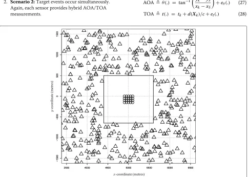
A sensor system, comprising of an array of 20 micro-phones, is deployed in order to detect and localise acoustic artillery firing events that occur within a two-dimensional geographical region (see Fig. 3).

Three scenarios are considered, given as follows:

1. Scenario 1:Target events occur at different times, with the time instance of each event sampled from a uniform distribution on [0, 100] seconds. Each sensor provides hybrid AOA/TOA measurements.

2. Scenario 2:Target events occur simultaneously. Again, each sensor provides hybrid AOA/TOA measurements.

3. Scenario 3:Target events occur simultaneously. Fifty percent of the sensors provide only AOA measurements, with the remaining sensors providing only TOA measurements.

In all scenarios, the number of false measurements gen-erated by each sensor has a Poisson distribution with mean 1.5×10−7 per square metre of the surveillance region. As a result, there are an average of 2.2 false mea-surements per sensor. Each false measurement is gener-ated at a random location uniformly distributed within the surveillance region. False alarms at different sensors are generated at different locations within the surveillance region. The parameter settings are summarised in Table 1.

4.2 Measurement generation 4.2.1 AOA and TOA measurements

Each sensor generates two-dimensional measurements of AOA (i.e. azimuth) and/or TOA of target events. If an event occurs at Cartesian coordinates Xk (xk,yk) at timetk, target-generated measurements (when they exist) are given as follows:

AOA θ(.) = tan−1

yk−yS xk−xS

+e_θ(.) (27)

TOA t(.) = tk+d(Xk)/c+et(.) (28)

(10)

Table 1Parameter values used in the simulations

Parameter Value

Number of sensors (N) 20

Locations of sensors Grid formation with separations of 50 m (see Fig. 1)

Probability of detection of each target (Pd) 0.8, 0.9, or 1.0

Average false alarms per sensor 2.2

AOA measurement error standard deviation (_σ_θ) 1o

DDOA measurement error standard deviation(√2cσt) 10 m

Signal propagation speed,c 343.2 m/s (i.e. the speed of sound in air)

Number of target events Up to 10

Target event locations Uniformly sampled in the surveillance region [3 km, 7 km]×[-2 km, 2 km], but excluding events from occurring within 500 m of the sensor array (again, see Fig. 3)

Target event times Either the same or each sampled from a uniform [0, 100] seconds distribution

whereeθ(.)andet(.), and zero-mean, Gaussian distributed measurement errors with standard deviations σθ andσt respectively;cis the signal propagation speed; andd(Xk) is the distance between the target and the sensor, i.e.:

d(Xk) =

(xk−xS)2+(yk−yS)2 (29)

where(xS,yS)are the Cartesian coordinates of the sensor.

4.2.2 DDOA measurement generation

Typically, the timestkat which the target events occur are unknown. However, these times can be factored out of the analysis by calculating the difference between the TOA measurements generated by different sensors (assuming the signal originates from the same target), giving mea-surements of the time difference of arrival (TDOA). Mul-tiplying the TDOA by the signal propagation speed, and under the assumption that the two TOA measurements are generated by the same target event, the distance dif-ference of arrival (DDOA) between TOA measurements generated by sensorsiandjis given as follows:

τ(i,j) ct(i)−t(j) (30) = di(Xk)−dj(Xk)

+cet(i)−et(j)

(31)

Importantly, Eq. (31) is independent oftk. The exploita-tion of TDOA measurements has been an area of great

interest for over three decades [33]. Each TDOA measure-ment provides a hyperbola of potential target locations, and the intersection of two such hyperbola enables the target location to be estimated (e.g. see [34]).

In determining the DDOA measurements, it is impor-tant to be aware of the potential for data incest (i.e. using the same information more than once), especially when one considers the following:

τ(i,k) = τ(i,j)+τ(j,k) (32)

In order to determine a unique set of DDOAs, in which no measurement is a linear combination of any of the other measurements, the DDOAs are calculated between a reference sensor (denoted throughout by the index “R”) and each of the other sensors. It is noted that the DDOA measurements generated by different sensors are corre-lated, because they utilise the same TOA measurement generated by the reference sensor. Indeed, it can easily be shown that Covτ(R,i),τ(R,j) = c2_σ2

t for i = j; and Cov[τ(R,i),τ(R,i)]=2c2_σ2

t fori=1,. . .,N.

The reference sensor is chosen to be the sensor at which the greatest number of measurements are generated. This ensures that the largest possible set of potential DDOA measurements is created. This is particularly important if there are missed detections, because in such cases a poor choice of reference sensor (i.e. choosing one at which very few measurements are generated) could severely restrict the number of DDOA measurement combinations eval-uated, which might negatively impact on the ability of the TALA to subsequently detect and localise the target events.

(11)

from the reverse triangle inequality that:

|dR(Xk)−di(Xk)| ≤

(xSR −xSi)2+(ySR−ySi)2 for alli

(33)

The inequality (33) states that the magnitude of each ground-truth DDOA measurement can be no greater than the distance between the reference sensor and sensori. Motivated by this, DDOA measurements are only consid-ered if they satisfy the following inequality:

|τ(R,i)| ≤

(xSR−xSi)2+(ySR−ySi)2+γ στ (34)

where στ √2cσt is the DDOA measurement error standard deviation; andγ ≥ 0 is a pre-specified multi-plier. Ifγ 1, DDOA measurements that do not satisfy Eq. (34) are likely to have been calculated from TOA measurements generated by different targets, although Eq. (34) can also be violated if TOA measurement errors are abnormally large.

4.3 TALA implementation

The TALA implementations in the three scenarios have the following features:

1. In scenarios 1–2, the TALA is implemented using the coupled AOA/DDOA measurement pairs, with the reference sensor providing only AOA measurements. 2. It is noted that the DDOA measurements

determined for different sensors are correlated, because they exploit the same TOA measurement set generated by the reference sensor. The correlation between between the DDOA measurements at different sensors isc2σ_t2. As a result, the matrix manipulations within the TALA cannot exploit the redundancy created had the measurement error covariance matrixbeen (block) diagonal5_.

3. In scenarios 1 and 3, initial candidate locations are generated as the intersection of each pair of AOA measurements and the intersection of each pair of DDOA measurements. Calculating the AOA

intersections is straightforward. However, calculating the DDOA intersections is more problematic, and an iterative N-R approach is used. Full details are given in Appendix A.

4. Scenario 2 is the most computationally complex because, respectively, the number of DDOA combinations that satisfy Eq. (34) is greater than in scenario 1, and the dimensionality of the

concatenated measurement vector is greater than in scenario 3. As a result, for scenario 2:

• Only the AOA intersections are used to generate initial candidate locations.

• The correlations between the DDOA

measurements are ignored (which simplifies the matrix manipulations within the TALA, e.g. see endnote 5).

5. In all three scenarios, in order to reduce the computational complexity of the TALA, the initial candidate locations are determined only from the intersections of measurements generated by five of the sensors.

6. In all three scenarios, deletion criterion 3 is used on Step 3. Therefore, the intersection deletion step only allows each AOA measurement to be exploited by one candidate location. As a result, in scenarios 1–2, the intersection deletion step must account for the fact that some AOA/DDOA measurement pairs share a common AOA measurement.

7. Only in scenario 3 is measurement reassociation performed during the G-N gradient descent.

A summary of the TALA settings is provided in Table 2. It is noted that some elements of the implementations (e.g. ignoring measurement correlations) can compro-mise algorithm performance for increased computational speed.

4.4 Performance evaluation

Results are based on 1000 simulations of each scenario; with either 1, 2,. . ., or 10 target events, and Pd values of 0.8, 0.9, and 1.0. In comparing the performance of the TALA with that of the gTALA and the CRLB, the overall location RMSE is calculated in each case. For the TALA, the overall location RMSE is given as follows:

overall location RMSE= NE total number of target events

detected (across the 1000 simulations) (38)

(12)

Table 2Summary of TALA settings

TALA component Details

AOA/DDOA intersections (Step 1) Based on measurements at only five sensors, only DDOAs satisfying Eq. (34) are used, withγ=2

N-R approach to determine DDOA intersections (Step 1) 10 attempts allowed: attempt #1 initialises with the corresponding AOA intersection, subsequent attempts use random starting locations

Measurement association (Step 2) Gate threshold,ξ=10−3(scenarios 1-2) gate threshold,ξ=10−2(scenarios 3)

Intersection downselection (Step 3) Only consider intersections for which the total number of associated measurements is no smaller thanNPd/2

G-N approach for ML estimation (Step 4) Determine overall likelihood for step sizes of_±20%,_±40%,_±60%,_±80%, and_±100% of the Newton step (i.e.m=5)

If no step increases the overall likelihood, consider a step of magnitude 200 m (i.e.

=δM) in a random direction

Stop iterating if the procedure above has attempted a total of 20 random steps, or each component of the GNSSEF(Xk)−1×

Z−f(Xk)

has a magnitude smaller than 10−3

Reassociation is only performed during gradient descent in scenario 3

The gTALA and CRLB overall location RMSEs are cal-culated in similar fashion, but do not require the pairing step because, in each case, the target event is pre-specified in each RMSE calculation. In order to reduce the impact of outliers, in Tables 3, 5, and 7, the overall location RMSEs are also calculated when the 1% worst geo-location esti-mates (in terms of the TALA overall location RMSE) are excluded from each calculation.

The percentage of target events detected (%E) and the average number of false events declared (#FE) are then given as follows:

%E = 100×NE/TE (39)

#FE = NFE/1000 (40)

where TE is the total number of events across the 1000 simulations, andNFE is the total number of false events declared across the 1000 simulations.

4.5 Simulation results

Simulation results are presented in Figs. 4, 5 and 6 and Tables 3, 4, 5, 6, 7 and 8. All simulations were run on an Intel®_{Core™i5-430M processor (2.26 GHz).}

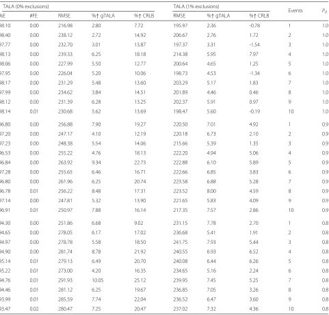
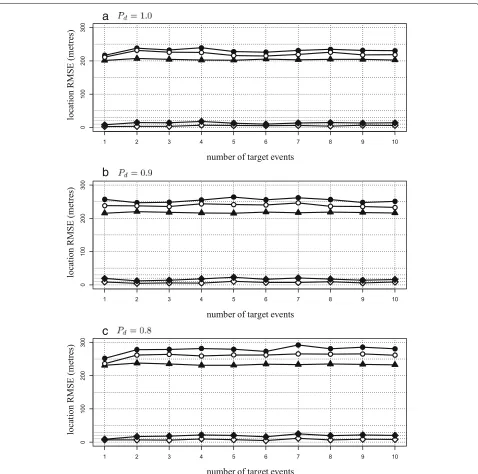
Firstly, in Fig. 4 and Table 3, the estimation accuracy of the TALA is shown for scenario 1. Estimation perfor-mance is similar to both the gTALA perforperfor-mance and the optimistic CRLB. Indeed, the RMSEs of the TALA and gTALA typically differ by less than 10%, indicating that the TALA is extremely good and making the correct asso-ciations of measurements to target events. In fact, the TALA makes the correct measurement-to-target associa-tion over 93% of the time in this scenario. Furthermore,

the RMSE of the TALA is typically within 10–20% of the CRLB. When outliers are removed from the analysis, dif-ferences in performance are even smaller, with the TALA RMSE typically around 5% greater than both the gTALA RMSE and the CRLB. The TALA is able to identify and geo-locate 93–98% of the target events (see column 1 in Table 3). Moreover, the average number of false events declared (i.e. estimates that are too geographically distant from a true target event to be considered to be detec-tion/localisation of an event) is negligible (see column 2 in Table 3).

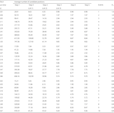
Table 4 shows the average computational time of the TALA for scenario 1. It is observed that for single events, the TALA provides almost instantaneous estimates. As the number of target events increases, the algorithm run-time increases exponentially, primarily because the num-ber of AOA and DDOA intersections that have to be computed and manipulated increases exponentially (see column 2). Nevertheless, the algorithm is still able to pro-vide estimates of the geo-locations of up to 10 target events in around 1 s.

(13)

Table 3Summary of the TALA geo-location performance for scenario 1

TALA (0% exclusions) TALA (1% exclusions)

Events Pd

%E #FE RMSE %_↑gTALA %_↑CRLB RMSE %_↑gTALA %_↑CRLB

98.10 0.00 216.98 2.80 7.72 195.97 2.36 -0.78 1 1.0

98.40 0.00 238.12 2.72 14.92 206.67 2.76 1.72 2 1.0

97.77 0.00 232.70 3.01 13.87 197.37 3.31 -1.54 3 1.0

98.13 0.00 239.33 6.25 18.18 214.38 5.95 7.97 4 1.0

98.06 0.00 227.99 5.50 12.77 200.64 4.65 1.25 5 1.0

97.95 0.00 226.04 5.20 10.06 198.73 4.53 -1.34 6 1.0

98.17 0.00 231.29 5.48 13.60 203.29 5.17 1.83 7 1.0

97.99 0.00 234.62 3.84 14.51 201.89 4.46 0.46 8 1.0

98.12 0.00 231.39 6.28 13.25 202.37 5.91 0.97 9 1.0

98.14 0.01 230.68 5.62 13.69 198.47 5.60 -0.19 10 1.0

96.80 0.00 256.88 7.90 19.27 220.50 7.01 4.92 1 0.9

97.20 0.00 247.17 4.10 12.19 220.18 6.73 2.10 2 0.9

97.23 0.00 248.38 5.54 14.06 215.66 5.39 1.35 3 0.9

96.53 0.00 255.22 4.76 18.13 222.20 4.94 5.06 4 0.9

96.84 0.00 263.92 9.34 22.73 222.88 6.10 5.89 5 0.9

97.28 0.00 255.65 6.46 16.71 222.66 6.85 3.83 6 0.9

96.80 0.00 261.96 6.25 20.74 223.58 6.88 5.28 7 0.9

96.78 0.01 256.22 8.48 17.31 223.52 8.00 4.59 8 0.9

97.14 0.00 247.81 5.32 13.90 221.65 5.83 4.09 9 0.9

96.91 0.01 250.97 7.88 16.14 217.35 7.57 2.86 10 0.9

94.30 0.00 251.86 6.68 9.02 231.15 7.78 2.70 1 0.8

94.65 0.00 278.05 6.17 17.02 236.68 5.41 1.91 2 0.8

94.97 0.00 278.78 5.58 18.50 241.75 7.93 5.44 3 0.8

94.90 0.00 281.74 8.78 21.92 240.55 6.93 6.52 4 0.8

95.14 0.01 279.13 6.49 20.70 240.08 6.44 6.26 5 0.8

95.22 0.01 273.00 4.20 16.35 234.65 5.16 2.24 6 0.8

94.76 0.01 291.93 10.05 25.12 239.95 7.45 5.25 7 0.8

94.46 0.01 281.12 6.25 19.67 236.85 7.05 3.26 8 0.8

93.99 0.01 285.59 7.74 22.04 236.52 6.47 3.60 9 0.8

93.47 0.02 280.47 7.25 20.47 237.02 7.32 4.36 10 0.8

Shown are the percentage of target events detected (%E), the average number of false events declared (#FE), and the geo-location RMSEs (in metres). RMSEs are shown for all target geo-geo-locations determined across the 1000 simulations (i.e. 0% exclusions), and with the worst 1% of geo-location estimates excluded from each RMSE calculation. Also shown are the percentage increase of the TALA RMSE over the gTALA RMSE (%↑gTALA) and the percentage increase of the TALA RMSE over the CRLB RMSE (%↑CRLB)

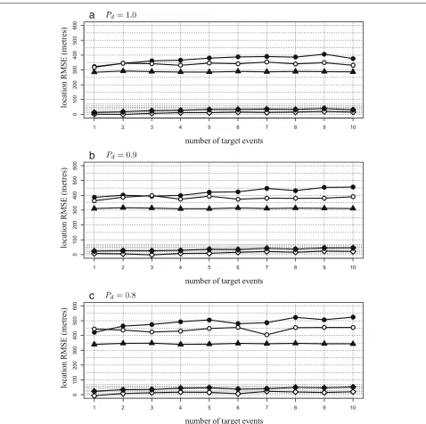
1. The geo-location performance of the TALA again compares well with the gTALA and the CRLB (see Fig. 5 and Table 5), with a degradation in

geo-location performance of just a few percent compared to scenario 1.

2. The TALA again detects 93–98% of the target events (see column 1 of Table 5).

3. The average number of false events declared is again negligible (see column 2 of Table 5).

4. The additional complexity of the data association problem has been negated by the changes to the TALA. As a result, in the most complex cases (i.e. with 10 target events), the TALA run-time remains less than 2 s (see Table 6).

(14)

a

b

c

Fig. 4Target localisation performance for scenario 1. The TALA RMSE (black circles), gTALA RMSE (white circles), and the CRLB RMSE (black triangles). The percentage differences between the performance of the TALA and (i) the CRLB (black diamonds) and (ii) the gTALA (white diamonds). Results are averaged over all 1000 simulations.aPd=1.0.bPd=0.9.cPd=0.8

occurring simultaneously, each sensor provides only AOA or TOA measurements, and not hybrid AOA/TOA mea-surements. This makes measurement association more problematic. For this reason, measurement reassocia-tion is performed on each iterareassocia-tion of the gradient descent algorithm, following the procedure described in Section 2.6.3. However, the reduced size of the concate-nated measurement vector, as a result of the reduction in the dimensionality of each measurement, does not

necessitate the computational adjustments to the TALA that were required for scenario 2.

(15)

a

b

c

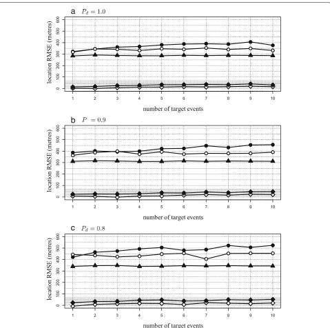
CRLB. When outliers are removed from the analysis, dif-ferences in performance are significantly reduced, with the TALA RMSE typically within 20% of both the gTALA RMSE and the CRLB. The TALA detects 83–99% of the target events (see column 1 of Table 7), whilst the average number of false events remains extremely low (see column 2 of Table 7). The reduced computational complexity of the algorithm, as a result of the reduction in the dimensionality of each concatenated measurement

vector, enables the TALA to generate estimates in the most complex scenarios in less than 0.5 s (see Table 8).

(16)

a

b

c

Conversely, setting the value of ξ too low can result in target-generated measurements failing to be gated. Via extensive experimentation in all three scenarios, thresh-old values in the range 10−3_{– 10}−2_{were shown to result} in near optimal performance. This is equivalent to gating the measurement Mahalanobis distance with a threshold gin the range 3.0–3.7.

The performance of the TALA was also assessed for both closely spaced and well separated emitters, and the

(17)

Table 4TALA average computational time, and the average number of candidate locations at the end of each step of the TALA, for scenario 1

TALA Average number of candidate positions

Events Pd

run time Step 1 Step 3 Step 3 Step 3 Step 4 Step 5

(s) (crit 1) (crit 2) (crit 3)

0.01 20.01 8.63 4.35 0.98 0.98 0.98 1 1.0

0.04 50.19 18.31 9.07 1.97 1.97 1.97 2 1.0

0.05 90.41 28.47 14.16 2.94 2.94 2.93 3 1.0

0.11 146.74 39.78 19.62 3.94 3.94 3.93 4 1.0

0.19 217.19 53.06 25.81 4.92 4.92 4.90 5 1.0

0.29 295.72 67.31 32.21 5.90 5.90 5.88 6 1.0

0.41 392.83 79.28 38.40 6.90 6.90 6.87 7 1.0

0.61 489.83 95.09 45.99 7.87 7.87 7.84 8 1.0

0.77 613.30 109.80 52.78 8.87 8.87 8.84 9 1.0

1.03 747.38 127.43 61.14 9.85 9.85 9.82 10 1.0

0.02 17.09 7.04 3.53 0.97 0.97 0.97 1 0.9

0.02 41.22 14.80 7.50 1.95 1.95 1.94 2 0.9

0.07 76.86 23.16 11.84 2.92 2.92 2.92 3 0.9

0.13 120.39 32.24 16.36 3.88 3.88 3.86 4 0.9

0.18 177.15 42.50 21.23 4.87 4.87 4.84 5 0.9

0.23 242.85 54.03 26.81 5.86 5.86 5.84 6 0.9

0.35 319.59 63.91 31.86 6.81 6.81 6.78 7 0.9

0.47 393.38 76.07 37.77 7.78 7.78 7.75 8 0.9

0.60 494.43 88.45 43.77 8.77 8.77 8.75 9 0.9

0.86 606.16 102.99 50.96 9.74 9.74 9.70 10 0.9

0.02 15.21 5.65 2.96 0.95 0.95 0.94 1 0.8

0.03 34.04 11.86 6.13 1.90 1.90 1.90 2 0.8

0.04 60.84 18.28 9.58 2.86 2.86 2.85 3 0.8

0.10 98.99 25.73 13.55 3.81 3.81 3.80 4 0.8

0.16 144.13 34.58 18.10 4.78 4.78 4.76 5 0.8

0.22 195.82 44.28 22.70 5.74 5.74 5.72 6 0.8

0.29 254.63 51.31 26.48 6.68 6.68 6.64 7 0.8

0.40 320.04 61.82 31.65 7.61 7.61 7.57 8 0.8

0.50 393.89 71.18 36.43 8.50 8.50 8.47 9 0.8

0.67 470.19 81.29 41.61 9.39 9.39 9.36 10 0.8

5 Discussion

There is a tradeoff between the run-time and the performance of the TALA. Adjustments that reduce the run-time, such as reducing the initial number of candidate locations (e.g. by not considering all mea-surement intersections), ignoring the correlations between DDOA measurements (e.g. to simplify the matrix manipulations in the gradient descent), and more quickly reducing the number of candidate loca-tions (e.g. by performing downselection on Step 3),

(18)

Events Pd

98.20 0.00 221.55 4.97 9.99 199.36 4.13 0.93 1 1.0

98.40 0.00 240.13 3.59 15.89 208.14 3.49 2.44 2 1.0

97.67 0.00 235.85 4.40 15.41 198.36 3.83 -1.05 3 1.0

98.02 0.00 240.26 6.67 18.65 214.88 6.20 8.23 4 1.0

97.72 0.00 227.59 5.31 12.57 203.19 5.98 2.54 5 1.0

97.73 0.00 230.52 7.29 12.24 202.06 6.28 0.32 6 1.0

97.86 0.00 233.17 6.34 14.53 204.34 5.71 2.35 7 1.0

97.75 0.00 236.42 4.63 15.39 203.31 5.19 1.17 8 1.0

97.83 0.00 235.20 8.03 15.11 204.10 6.82 1.83 9 1.0

97.76 0.00 235.39 7.78 16.02 202.92 7.96 2.04 10 1.0

96.60 0.00 261.04 9.65 21.20 222.55 8.01 5.89 1 0.9

97.20 0.00 248.90 4.82 12.97 221.57 7.40 2.75 2 0.9

97.00 0.00 250.68 6.52 15.11 219.06 7.06 2.95 3 0.9

96.60 0.00 260.54 6.95 20.60 227.29 7.34 7.47 4 0.9

96.50 0.01 262.33 8.68 21.99 225.08 7.15 6.94 5 0.9

97.08 0.00 259.16 7.92 18.31 224.81 7.88 4.84 6 0.9

96.49 0.00 264.01 7.08 21.68 226.14 8.10 6.49 7 0.9

96.38 0.01 262.57 11.17 20.22 227.18 9.76 6.30 8 0.9

96.66 0.01 253.79 7.86 16.65 226.42 8.10 6.33 9 0.9

96.25 0.01 257.98 10.90 19.39 221.94 9.84 5.04 10 0.9

94.30 0.00 251.48 6.52 8.85 232.14 8.24 3.14 1 0.8

94.45 0.01 284.93 8.80 19.91 238.50 6.22 2.69 2 0.8

95.00 0.00 285.47 8.11 21.34 246.61 10.10 7.56 3 0.8

94.55 0.00 287.55 11.02 24.43 244.97 8.90 8.48 4 0.8

94.74 0.01 289.19 10.32 25.05 239.86 6.35 6.17 5 0.8

94.87 0.01 277.23 5.81 18.15 238.06 6.69 3.72 6 0.8

94.34 0.01 290.23 9.41 24.39 243.57 9.08 6.84 7 0.8

94.03 0.02 290.22 9.69 23.54 241.85 9.31 5.43 8 0.8

93.38 0.02 288.33 8.77 23.21 240.69 8.35 5.42 9 0.8

92.60 0.02 289.14 10.56 24.19 240.79 9.03 6.02 10 0.8

Again, shown are the percentage of target events detected (%E), the average number of false events declared (#FE), and the geo-location RMSEs (in metres). RMSEs are shown for all target geo-locations determined across the 1000 simulations (i.e. 0% exclusions), and with the worst 1% of geo-location estimates excluded from each RMSE calculation. Again, also shown are the percentage increase of the TALA RMSE over the gTALA RMSE (%↑gTALA) and the percentage increase of the TALA RMSE over the CRLB RMSE (%↑CRLB)

Deciding when it is necessary to make computational simplifications can be performed “on-the-fly”, based on the number of measurements generated within the time window under consideration. A larger number of mea-surements may indicate a large number of emitters and/or signals that are closely spaced in time, which may then necessitate computational savings. Of course, the algorith-mic complexity that can be afforded depends on the time-criticality of the application, specifically whether the

com-mander requires the processing to be performed almost instantaneously (e.g. in order to immediately perform a retaliatory strike), or whether a longer processing time can be tolerated (e.g. when conducting post-event analysis).

6 Future work

(19)

Events Pd

0.01 20.60 8.14 4.00 0.98 0.98 0.98 1 1.0

0.01 53.16 17.36 8.36 1.97 1.97 1.97 2 1.0

0.02 95.94 27.17 13.19 2.94 2.94 2.93 3 1.0

0.07 157.20 38.03 18.28 3.94 3.94 3.92 4 1.0

0.14 224.86 50.44 23.96 4.91 4.91 4.89 5 1.0

0.23 303.82 63.97 29.81 5.89 5.89 5.87 6 1.0

0.42 397.65 75.00 35.38 6.88 6.88 6.85 7 1.0

0.63 494.44 90.18 42.58 7.85 7.85 7.82 8 1.0

0.98 602.77 103.05 48.20 8.84 8.84 8.81 9 1.0

1.53 731.13 119.31 55.76 9.81 9.81 9.78 10 1.0

0.00 17.70 6.64 3.24 0.97 0.97 0.97 1 0.9

0.01 44.37 14.07 6.96 1.95 1.95 1.94 2 0.9

0.02 82.47 22.38 11.20 2.92 2.92 2.91 3 0.9

0.05 129.90 31.09 15.43 3.88 3.88 3.87 4 0.9

0.11 186.77 41.34 20.24 4.85 4.85 4.83 5 0.9

0.20 253.62 52.50 25.55 5.85 5.85 5.83 6 0.9

0.34 330.56 62.03 30.28 6.79 6.79 6.76 7 0.9

0.49 406.79 74.07 36.12 7.75 7.75 7.72 8 0.9

0.73 500.82 85.82 41.60 8.72 8.72 8.70 9 0.9

1.08 603.86 99.32 48.15 9.68 9.68 9.64 10 0.9

0.00 15.82 5.38 2.77 0.95 0.95 0.94 1 0.8

0.01 37.45 11.43 5.76 1.90 1.90 1.89 2 0.8

0.01 68.19 17.84 9.18 2.87 2.87 2.85 3 0.8

0.02 110.12 25.08 13.02 3.80 3.80 3.79 4 0.8

0.09 158.49 33.88 17.42 4.76 4.76 4.74 5 0.8

0.16 213.10 43.44 21.94 5.72 5.72 5.70 6 0.8

0.24 273.47 50.27 25.60 6.65 6.65 6.61 7 0.8

0.39 340.90 60.32 30.59 7.58 7.58 7.54 8 0.8

0.52 415.07 69.45 35.09 8.45 8.45 8.42 9 0.8

0.76 495.93 79.54 40.03 9.31 9.31 9.28 10 0.8

used in deletion criterion 1 on Step 3, and (iii):γ >0 in Eq. (34). The performance of the TALA is also dependent on the measurement errors (i.e.σ_θandσt

in the focal simulations). It would be interesting to analyse the performance of the TALA as a function of these parameters, in order to determine optimal values for the heuristic parameters as a function of the measurement errors. Such an analysis may offer valuable insight into how to optimise the

performance of the TALA across a broad range of operational scenarios.

2. The performance of the TALA was compared to both the CRLB [23] and the performance of a “genie” TALA that exploited the true measurement-to-target associations. It would be interesting to compare the performance of the TALA to that of existing methods developed for specific applications, most notably the approaches of [2, 10, 19, 20] developed for multi-target localisation using TOA

(20)

Events Pd

98.80 0.00 322.48 1.35 13.32 288.98 2.88 3.74 1 1.0

97.95 0.00 345.15 0.13 17.89 297.41 2.14 3.58 2 1.0

97.07 0.01 361.52 5.67 25.05 290.89 3.33 2.52 3 1.0

95.23 0.01 366.09 10.33 27.86 307.61 6.49 9.54 4 1.0

94.52 0.01 379.98 9.55 32.95 310.85 9.98 10.97 5 1.0

93.05 0.01 387.99 13.53 33.68 317.57 12.24 11.60 6 1.0

93.01 0.02 390.64 10.55 35.78 313.90 10.25 11.27 7 1.0

91.60 0.02 386.88 13.69 33.54 309.56 10.31 8.95 8 1.0

91.17 0.03 406.21 16.30 40.65 325.19 11.81 14.79 9 1.0

89.81 0.03 376.56 13.63 31.32 315.84 13.47 12.36 10 1.0

98.10 0.00 386.89 6.51 24.38 320.99 6.38 6.05 1 0.9

96.10 0.01 401.60 3.73 26.66 330.65 5.99 6.90 2 0.9

95.63 0.01 394.15 -1.23 25.29 327.46 3.16 7.42 3 0.9

93.13 0.02 399.20 6.69 28.96 326.57 8.49 8.00 4 0.9

92.18 0.01 421.33 6.91 36.20 339.06 6.76 12.38 5 0.9

89.65 0.03 423.84 13.28 34.23 341.83 10.26 11.17 6 0.9

90.30 0.03 446.99 17.38 43.35 350.90 12.17 15.52 7 0.9

88.42 0.03 431.47 13.49 37.18 345.19 12.75 12.70 8 0.9

87.40 0.04 453.87 19.29 44.99 360.63 15.51 18.17 9 0.9

86.34 0.04 456.16 16.64 46.35 353.35 17.47 16.77 10 0.9

94.00 0.01 421.12 -5.11 23.97 359.77 4.31 10.18 1 0.8

94.15 0.02 464.01 6.32 33.56 366.50 6.98 9.12 2 0.8

91.73 0.02 473.74 11.72 36.06 377.14 9.41 12.75 3 0.8

90.22 0.03 492.75 14.66 45.12 381.17 13.08 15.81 4 0.8

88.86 0.04 504.91 12.79 47.65 392.40 13.57 18.91 5 0.8

86.60 0.05 479.99 5.59 38.64 385.92 9.54 15.16 6 0.8

86.80 0.06 486.42 20.15 41.21 382.79 15.62 15.09 7 0.8

85.00 0.05 522.25 15.20 50.37 397.93 14.58 18.81 8 0.8

83.92 0.07 506.22 11.31 47.08 401.54 17.14 20.90 9 0.8

83.08 0.08 524.07 15.39 52.56 404.82 19.72 22.49 10 0.8

Again, shown are the percentage of target events detected (%E), the average number of false events declared (#FE), and the geo-location RMSEs (in metres). RMSEs are shown for all target geo-locations determined across the 1000 simulations (i.e. 0% exclusions), and with the worst 1% of geo-location estimates excluded from each RMSE calculation. Again, also shown are the percentage increase of the TALA RMSE over the gTALA RMSE (%↑gTALA) and the percentage increase of the TALA RMSE over the CRLB RMSE (%↑CRLB)

3. The TALA implementation introduced herein implicitly assumes that the measurement error standard deviations are known. Extensive field testing of a prototype system may enable accurate error statistics to be determined, making this a valid assumption. In cases for which field testing is not practicable, or in extended operating conditions, measurement error standard deviations may not be

(21)

Events Pd

0.01 55.53 10.05 5.04 1.01 1.01 0.99 1 1.0

0.01 97.69 22.35 11.86 2.01 1.99 1.96 2 1.0

0.04 149.39 35.80 20.03 3.00 2.98 2.92 3 1.0

0.03 215.67 53.84 31.83 3.94 3.92 3.82 4 1.0

0.08 284.31 76.63 47.35 4.91 4.88 4.74 5 1.0

0.12 368.60 102.52 65.49 5.83 5.79 5.59 6 1.0

0.17 463.94 130.97 86.62 6.77 6.72 6.53 7 1.0

0.24 563.94 171.32 116.61 7.69 7.63 7.35 8 1.0

0.33 674.47 213.64 149.62 8.62 8.55 8.24 9 1.0

0.43 803.40 267.18 191.98 9.48 9.40 9.01 10 1.0

0.01 52.12 8.24 4.18 1.02 1.01 0.98 1 0.9

0.02 89.31 17.86 9.72 1.99 1.96 1.93 2 0.9

0.02 134.80 28.85 16.10 2.96 2.93 2.88 3 0.9

0.04 187.96 42.65 25.40 3.88 3.83 3.74 4 0.9

0.04 247.24 60.20 37.14 4.81 4.75 4.62 5 0.9

0.13 318.68 79.85 51.03 5.67 5.58 5.40 6 0.9

0.17 396.73 102.12 67.94 6.61 6.53 6.35 7 0.9

0.24 476.01 129.76 88.87 7.46 7.38 7.11 8 0.9

0.31 571.35 163.07 114.19 8.30 8.20 7.91 9 0.9

0.41 674.19 204.32 147.04 9.18 9.07 8.67 10 0.9

0.01 50.18 8.90 5.22 1.21 1.18 0.95 1 0.8

0.01 81.14 19.47 11.79 2.18 2.14 1.90 2 0.8

0.01 116.63 31.50 20.02 3.11 3.04 2.77 3 0.8

0.03 162.80 48.00 31.80 4.05 3.97 3.64 4 0.8

0.05 214.78 71.33 48.32 4.94 4.85 4.48 5 0.8

0.11 272.45 95.83 66.88 5.82 5.70 5.25 6 0.8

0.17 330.48 122.64 87.85 6.74 6.59 6.13 7 0.8

0.20 401.28 160.11 116.92 7.60 7.45 6.85 8 0.8

0.27 477.67 201.82 149.49 8.40 8.26 7.63 9 0.8

0.36 564.86 250.12 188.52 9.28 9.11 8.38 10 0.8

7 Conclusions

In this paper, a novel target acquisition and localisation algorithm (TALA) has been introduced that offers a capa-bility for detecting and localising an unknown number of targets using the intermittent “signals-of-opportunity” they generate (e.g. “events” such as acoustic impulses or radio frequency transmissions). The TALA is a batch estimator, and its novelty lies in the mechanism by which it circumnavigates the need to perform global

(22)

location. The algorithm then determines maximum like-lihood estimates of potential target locations, before a final downselection step ensures that each measurement is associated with no greater than one estimate.

The performance of the TALA is demonstrated for simulated scenarios with a network of 20 sensors and up to 10 targets. The sensors generate angle-of-arrival (AOA), time-of-arrival (TOA), or hybrid AOA/TOA mea-surements. Both simultaneous and non-simultaneous tar-get events are considered, though clearly simultaneous events are more challenging, as the problem of resolv-ing the association of measurements to events has greater ambiguity.

For non-simultaneous events, and with homogeneous sensors providing hybrid AOA/TOA measurements, the target localisation errors of the TALA are typically within 10–20% of an optimistic Cramér-Rao lower bound (CRLB) that ignores the multi-target data association problem. A better comparison shows that the local-isation errors of the TALA are typically within 10% of the errors generated by a “genie” algorithm that is given the correct measurement-to-target associations. Percentage differences in performance are reduced when a small percentage (i.e. 1%) of outliers are removed from the comparisons, with the TALA RMSE typi-cally then around 5% greater than both the gTALA RMSE and the CRLB. For simultaneous events, again with sensors providing hybrid AOA/TOA measurements, there is only a few percent degradation in geo-location performance compared to the case of non-simultaneous events. In both cases, the TALA successfully detect 93–98% of the targets, with virtually no false targets declared.

In the most difficult scenarios considered, with simulta-neous events, and heterogesimulta-neous sensors providing either AOA or TOA measurements, the TALA continues to per-form well in comparison to the gTALA and the optimistic CRLB. To elaborate, in this case, the RMSEs of the TALA and gTALA typically differ by 10–20%, with the RMSE of the TALA typically 20–50% greater the CRLB. Again, when outliers are removed from the analysis, differences in performance are reduced significantly, with the TALA RMSE typically within 20% of the CRLB. The TALA detects 83–99% of the target events, whilst the average number of false events remains extremely low.

The computational expense of the TALA is shown to remain manageable as the number of targets increases. This allows the approach to be implemented in challeng-ing time-critical scenarios, such as in the localisation of artillery firing events, for which there may be only a small window of opportunity in which to perform a retaliatory strike. It is concluded that the TALA provides a pow-erful situational awareness aid for passive surveillance operations.

Endnotes

1_{This is a common assumption in target state}

estima-tion problems (e.g. see [22]). For scenarios in which this assumption is violated, there are two options; either (i) a Gaussian approximation can be made or (ii) the likelihood functions and ML estimation approach within the TALA be modified in order to correctly account for the change in the measurement model.

2_{The maximum value of the individual likelihood is}

li(max)=det(i)−1/2/(2π)di/2.

3_{Via experimentation, likelihood threshold values}_ξ _in

the range 10−3– 10−2were shown to generate excellent results. At the ML estimate, the GNSSE has a value of 0.

5_{For example, if the measurement error covariance}

matrixwere block diagonal, it can easily be shown that

F(Xk)−1[Z−f(Xk)]= ment error covariance matrix (given in Eq. (13)) has complexityO(N_a3).

Appendix A: Determining the AOA and DDOA measurement intersections

AOA intersections

Consider two AOA measurementsθ(i)generated by sen-sorsi=1, 2. It is straightforward to show that the point of intersection(xI,yI)of these two measurements is given as follows:

wherexandyare the distances between the two sen-sors in the x- andy- coordinate directions respectively, i.e.