OpenSWPC: an open source integrated parallel simulation code for modeling seismic wave propagation in 3D heterogeneous viscoelastic media

TECHNICAL REPORT

OpenSWPC: an open-source integrated

parallel simulation code for modeling seismic

wave propagation in 3D heterogeneous

viscoelastic media

Takuto Maeda

_{, Shunsuke Takemura}

_{and Takashi Furumura}

Abstract

We have developed an open-source software package, Open-source Seismic Wave Propagation Code (OpenSWPC), for parallel numerical simulations of seismic wave propagation in 3D and 2D (P-SV and SH) viscoelastic media based on the finite difference method in local-to-regional scales. This code is equipped with a frequency-independent attenuation model based on the generalized Zener body and an efficient perfectly matched layer for absorbing boundary condition. A hybrid-style programming using OpenMP and the Message Passing Interface (MPI) is adopted for efficient parallel computation. OpenSWPC has wide applicability for seismological studies and great portability to allowing excellent performance from PC clusters to supercomputers. Without modifying the code, users can conduct seismic wave propagation simulations using their own velocity structure models and the necessary source represen-tations by specifying them in an input parameter file. The code has various modes for different types of velocity struc-ture model input and different source representations such as single force, moment tensor and plane-wave incidence, which can easily be selected via the input parameters. Widely used binary data formats, the Network Common Data Form (NetCDF) and the Seismic Analysis Code (SAC) are adopted for the input of the heterogeneous structure model and the outputs of the simulation results, so users can easily handle the input/output datasets. All codes are written in Fortran 2003 and are available with detailed documents in a public repository.

Keywords: Seismic waves, Numerical simulation, Finite difference method, Parallel computing, Open-source software

© The Author(s) 2017. This article is distributed under the terms of the Creative Commons Attribution 4.0 International License (http://creativecommons.org/licenses/by/4.0/), which permits unrestricted use, distribution, and reproduction in any medium, provided you give appropriate credit to the original author(s) and the source, provide a link to the Creative Commons license, and indicate if changes were made.

Background

The numerical simulation of seismic wave propagation is a fundamental tool for seismological studies such as estimation of the heterogeneous velocity structure (e.g., Tape et al. 2009; Chen and Lee 2015), the study of seis-mic source processes (e.g., Lee et al. 2006; Imperatori and Gallovič 2017), wave propagation in the heterogeneous Earth (e.g., Frankel and Clayton 1986; Emoto et al. 2010) and hazard assessment (e.g., Graves et  al. 2010; Maeda et al. 2016). Significant improvements in numerical sim-ulation techniques, high-resolution velocity structure

models and high-performance computer systems have enabled the use of 3D numerical simulations as a practi-cal tool for regular data processing studies with currently available parallel computers.

Of the wide variety of numerical methods used to simulate seismic wave propagation, the staggered-grid finite difference method (FDM) has been widely used in the seismological community. The staggered-grid FDM with second-order accuracy in space and time to simulate seismic waves was first proposed by Madariaga (1976); then, it was expanded to fourth-order accuracy in space by Levander (1988). The 3D FDM simulation of seismic wave propagation at regional scales has been conducted after Olsen et  al. (1995) and Graves (1996). Since then, the FDM simulations have been widely used for the numerical modeling of seismic wave propagation

Open Access

*Correspondence: maeda@eri.u-tokyo.ac.jp

1 _{Earthquake Research Institute, The University of Tokyo, 1-1-1 Yayoi,} Bunkyo 113-0032, Tokyo, Japan

(see Moczo et  al. 2014 and references therein) due to the relative simplicity of its numerical algorithm as well as its computational efficiency in parallel computing. Multiple available FDM codes, such as GMS (Aoi and Fujiwara 1999; Aoi et  al. 2004), FDMPI (Bohlen 2002), AWP-ODC (Cui et al. 2013), FDSim (Moczo et al. 2014) and SW4 (Petersson and Sjogreen 2014), have been used to numerically model seismic wave propagation. Many other available community codes including other numerical methods such as the spectral-element method are described in Igel (2016).

In this study, we developed a new staggered-grid FDM code to model seismic waves in 3D and 2D viscoelastic media in local-to-regional scale. By improving the usa-bility of the code, called the Open-source Seismic Wave Propagation Code (OpenSWPC), the numerical simula-tion with parallel computing of a wide variety of targets is made accessible to users. The original version of this code, designed to be implemented on supercomputers (Furumura and Chen 2005; Inoue et al. 2013), was fully restructured to have excellent performance on a variety of computer architectures to be fully open to the seismo-logical community.

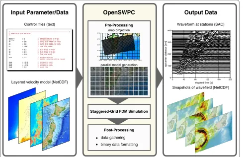
The development of OpenSWPC was in particular intended to improve its usability for non-experts who are not so familiar with numerical simulation techniques. For this purpose, OpenSWPC combines the necessary pre- and post-processing functions in its main simu-lation code (Fig. 1), and all the necessity information for the simulations are defined in input text parameter files. Therefore, users do not need to modify the code to apply it to individual simulation targets. We adopt de facto standard formats for the binary input and out-put datasets; the velocity structure inout-put model is given in the Network Common Data Form (NetCDF; Rew and Davis 1990), and the simulation results are output in the NetCDF and the Seismic Analysis Code (SAC; Goldstein et al. 2003; Helffrich et al. 2013) formats. Following the input parameters, OpenSWPC dynamically allocates the computer memory, automatically generates grids for a heterogeneous velocity model and performs parallel numerical simulations of seismic wave propagation.

In the following, we briefly review the strategy of the FDM simulation of seismic wave propagation in hetero-geneous viscoelastic media with frequency-independent attenuation and the numerical techniques adopted in the

Input Parameter/Data

Controll files (text)

OpenSWPC

Layered velocity model (NetCDF)

128˚E129˚E130˚E131˚E132˚E133˚E134˚E135˚E136˚E 30˚N

31˚N 32˚N 33˚N 34˚N

Pre-Processing map projection

parallel model generation

Staggered-Grid FDM Simulation

Post-Processing data gathering binary data formatting

Output Data

Waveform at stations (SAC)

Snapshots of wavefield (NetCDF) 0

100 200 300 400

epicenter distance [km

]

elapsed time [s]

200 160 120 80 40 0

present code. Then, examples of numerical simulations are demonstrated to show how the present code works.

Methods

In this section, we briefly introduce the staggered-grid FDM method for simulating seismic waves in viscoelastic media and the algorithms adopted in OpenSWPC. The details of theories for viscoelasticity and numerical algo-rithms can be found in Moczo et al. (2014) and Igel (2016).

Seismic wave modeling with a viscoelastic body

We solve the equation of motion of continuum mechan-ics described by the velocity and stress components in the Cartesian coordinate system such that

where ND is the model dimension (ND=2 or 3), vi is the particle velocity of the elastic motion in the ith compo-nent, ρ is the density, σij is the i, jth component of the

stress tensor and fi is the ith component of the body

force. In the following, we primarily describe the three-dimensional case, ND=3; however, it is straightforward to reproduce the two-dimensional P-SV or SH formulae from this case.

The stress is related to the particle velocity via the con-stitutive equation. In this study, we adopted the General-ized Zener Body (GZB) (e.g., JafarGandomi and Takenaka

2007; Maeda et  al. 2013) of the viscoelasticity, which is expressed as a parallel connection of Zener bodies (e.g., Aki and Richards 2002, Chapter 5) having different physi-cal constants. Note that the GZB is known to be equiva-lent to the generalized Maxwell body (Moczo and Kristek

2005; Cao and Yin 2014), which is also widely used for seismic wave modeling (e.g., Emmerich and Korn 1987).

Following Robertsson et  al. (1994), the constitutive equation of the viscoelastic body is written as

where ǫij is the i, jth component of the strain tensor, ψ˙π(t) and ψ˙µ(t) are the time derivatives of the relaxation

func-tions for two independent relaxed moduli πR≡R+µR and µR, respectively. For the GZB, they are represented using the L different relaxation times τ_ℓσ (ℓ=1,. . .,L )

As a consequence of introducing the viscoelasticity, the phase speeds of the body waves become a function of the frequency due to the physical dispersion effect (Aki and Richards 2002). Therefore, they follow the given velocity structure at a given reference frequency fR.

In the actual Earth medium, QP and QS do not

signifi-cantly depend on frequency over a wide frequency range below ∼1 Hz. To yield an approximately constant Q over a frequency range, we introduced memory variables fol-lowing Robertsson et al. (1994) with the τ-method pro-posed by Blanch et al. (1995). The τ-method assumes that

the ratios between the relaxation and creep times are constant among all Zener bodies (ℓ=1,. . .,L):

From a given set of relaxation times, the τ-method gives

optimized values for the parameters τP and τS using the least squares method, so that the attenuation QP and QS

become approximately constant over a given frequency range. The constitutive equation based on this τ-method is written as follows:

where rijℓ is the memory variable of the (i, j)th

compo-nent of the stress tensor and the ℓth Zener body and sat-isfy the following auxiliary equation:

The selection of the relaxation times, τ_ℓσ, is not a

an approximately constant Q over two orders of the frequency range below 2 Hz using three Zener bodies (L₌3). Frequency range of the approximately constant

Q is adjustable by input parameter of the code.

Discretization

The equation of motion, Eq. (1), and the constitutive equations, Eqs. (5) and (6), are solved numerically based on a staggered-grid FDM with fourth-order accuracy in space and second-order accuracy in time (e.g., Levander

1988). We adopt the Cartesian coordinate system with

x1=x and x2=y as the horizontal direction and vertical

axis x3=z was taken to be positive downward with aver-age sea level height at z₌0. Figure 3 shows the layout of

the staggered-grid adopted in this study.

We adopted the first-order Crank–Nicolson method to calculate the time integration of the constitutive equa-tion, Eq. (5), and the auxiliary equation for the memory variables, Eq.  (6). This enables us to solve the original implicit scheme equations explicitly. The discretized for-mula can be found in Maeda et al. (2013).

The evaluation of the medium properties defined in the staggered-grid system requires appropriate averag-ing of the medium parameters defined on the neighbor-ing grids. In this code, all medium properties (relaxed medium parameters _R and _µR, density _ρ, and attenuation parameters τP and τS) are defined on the same grid as

the normal stress components (Fig. 3). Averaging of the density on neighboring grids is necessary when evaluat-ing the velocity, Eq. (1), and averaging the relaxed rigidity

modulus is necessary when evaluating the shear stress components and the accompanying memory variables (Eqs. 5, 6). For the averaging, we adopted an arithmetic and a harmonic averaging for the density and the relaxed rigidity modulus, respectively. Notice that no averaging is necessary for _R because it is used only for updating the normal stress components.

Boundary conditions

The free surface and ocean bottom boundary condi-tions are implemented in the FDM simulation based on the efficient Heterogeneity, Oceanic layer and Topogra-phy (HOT) FDM method (Nakamura et  al. 2012). This method was originally developed for a second-order FDM method to include the topographic variations of volcanoes (Ohminato and Chouet 1997). Later, it was shown that this condition could be applied effectively for fluid–solid boundaries (Okamoto and Takenaka 2005). Currently, HOT-FDM is widely applied in regional-scale modeling of seismic wave propagation in coastal areas (e.g., Maeda and Furumura 2013; Maeda et al. 2013, 2014; Nakamura et al. 2012, 2015; Noguchi et al. 2016; Todoriki et al. 2017), in high-frequency seismic wave simulations of topographic scattering (Takemura et al. 2015), and in the synthesis of elastic wave propagation in cylinder-shaped materials on the scale of 10 cm (Yoshimitsu et al. 2016), demonstrating the ability of the HOT-FDM to include irregular topography and curved surfaces in FDM.

In this HOT-FDM method, the air column is treated as a medium with a very small density and zero wavespeeds for the P- and S-waves as αR=βR=0 [km/s]. This

col-umn is treated as a vacuum where no seismic wave can propagate due to zero wavespeeds. The ocean column is treated as an elastic medium having ρ₌1.0  [g/cm3], 0.0002

0.0005 0.001 0.002 0.005 0.01 0.02

Q

−1

10−3 ₁₀−2 ₁₀−1 ₁₀0 ₁₀1 ₁₀2

frequency [Hz]

Fig. 2 An example of a nearly constant Q model using three Zener bodies (bold black curve), considering a constant Q (=100) in the frequency range between 0.02 and 2 Hz. Dotted lines show the contri-butions from three Zener bodies

vx vy

σii

σxy

σyz σxz

x y z vz

αR=1.5 [km/s] and βR=0.0 [km/s]. On the free surface

and seafloor, a reduced, second-order FDM scheme is applied instead of the fourth-order FDM. To apply such a reduced-order FDM across the boundaries, the location of the boundaries are detected automatically in Open-SWPC by searching for the grid positions where µR and

_R change from zero to a finite value.

Except in whole-Earth seismic wave modeling, an appropriate absorbing boundary condition surrounding the bounded model is necessary to avoid artificial reflec-tions from the boundaries of the computational model. We adopt the Perfectly Matched Layer (PML) boundary condition (after Chew and Liu 2011) to minimize artifi-cial reflections. Up to now, various PML methods have been developed (for example, Kristek et  al. 2009 and references therein); we adopted an implementation pro-posed by Zhang and Shen (2010) to consider its effective-ness in and applicability to OpenSWPC.

This PML method solves the auxiliary differential equa-tions in addition to the equaequa-tions of motion and the con-stitutive equations in the absorbing zone with complex and frequency-shifted absorbing functions. Typically 10–20 grids are used for the thickness of the PML zone surrounding the model; this can be defined in the input parameters. To avoid large computational loads when solving the auxiliary equations of the PML, we assumed that the material in the PML zone was perfectly elastic and did not calculate the memory variables (Eq. 6), for the anelasticity.

Even though the PML efficiently absorbs outgoing waves from the model, it occasionally causes severe instabilities during the calculation, in particular when the seismic waves propagate in highly heterogeneous structures with very large velocity contrasts (Maeda et al.

2013). Therefore, we also implemented the stable sponge boundary condition of Cerjan et al. (1985), which simply attenuates the waves in the absorbing layer by multiply-ing small values to the stress and velocity components in the absorbing zone at each time step so that users can select the appropriate boundary condition. Note that the sponge condition is perfectly stable but less efficient when absorbing outgoing waves.

Seismic source representation

The seismic moment tensor source can be implemented in the FDM either by couples of body forces (Graves

1996) or based on a stress discontinuity representa-tion (Coutant et al. 1995; Pitarka 1999). In OpenSWPC, the stress discontinuity representation was adopted to implement the moment tensor sources. The seismic source can be implemented in OpenSWPC with a sin-gle point source. A finite-fault source can be represented

using multiple point sources (Graves and Wald 2001; Takenaka and Fujii 2008). In this code, there is no restriction on the number of point sources; the code automatically detects the number of sources and allo-cates the required memory. We also implemented a sin-gle-force source that is widely used for modeling seismic signals excited in volcanic environments (e.g., Ohmi-nato et al. 1998). Both moment tensor and single-force sources are placed on the nearest grid point of the nor-mal stress component. This source grid point is averaged with the neighboring source grid points if necessary when updating the shear stress and velocity components (Coutant et al. 1995).

The seismic source time function is represented by bell-like functions (Fig. 4) of various forms such as box-car, triangle and cosine functions, Herrmann’s quadratic function (Herrmann 1979) and Küpper’s wavelet of a sin-gle cycle (Mavroeidis and Papageorgiou 2003). They have a common cutoff frequency, which is a reciprocal of the source duration time, but have different roll-offs above the cutoff frequency.

The incidence of plane P- or S-waves with near-vertical angles was also implemented in OpenSWPC. The plane-wave incidence uses a solution of the up-going plane-wave of the 1D wave equation in a homogeneous medium as an initial condition of the velocity and stress components at the bottom of the model (e.g., Emoto et  al. 2010). A bell-like-shaped spatial distribution corresponding to the source time function (Fig. 4) is assumed as initial condi-tions. Even though the OpenSWPC allows a non-vertical incidence angle to be set for the plane wave, note that artificial reflections may arise at both sides of the plane wave traveling in the absorbing boundaries with increas-ing plane-wave incidence angles.

Simulations exchanging source and station positions are sometimes conducted because the reciprocity theo-rem (e.g., Aki and Richards 2002) implies the equivalence of both simulation results under certain conditions. The use of the reciprocity theorem is very effective to obtain a large number of synthetic seismograms for a small number of stations when there is a very large number of source grids, e.g., when calculating Green’s function with reduced computational cost (e.g., Graves and Wald 2001; Eisner and Clayton 2001; Zhao et  al. 2006; Hsieh et  al.

Software implementations

Parallel computing

All codes in OpenSWPC were written following to the standards of Fortran 2003 (e.g., Adams et al. 2008) with very few compiler-unique functions; therefore, this code should work in a variety of computational environ-ments without modification. This code uses the external

libraries of Message Passing Interface (MPI) and NetCDF for parallel computing and data I/O, respectively. Note that these external libraries also work in many environments.

In OpenSWPC, all definitions such as parallelization strategies, model size, discretization and output file-names are defined in the input parameter files. Because

0

the computational memory is allocated dynamically, users do not need to re-compile the code to perform simula-tions with different model sizes. OpenSWPC adopts a domain-partitioning procedure for the parallel comput-ing uscomput-ing MPI. It performs 2D and 1D model partition-ing in the horizontal directions for the 3D and 2D codes, respectively (see Fig. 5 for the partitioning for the 3D code). Then, OpenSWPC sets up the velocity structure model for the partitioned domain on each CPU or CPU core, and calculates the seismic wave propagation in the domain using MPI data communication at each time step.

To maintain wavefield continuities across the par-titioned domain, the velocity and stress components defined at the two-point-thick outermost layer are exchanged with those of the neighboring partitioned domains at every time step using MPI (Fig. 5b). We adopted hybrid-style programming using OpenMP and MPI (e.g., Furumura and Chen 2005) to make full use of many CPUs with multiple CPU cores; directive-based OpenMP parallel programming is applied to parallel-ize the computation among the CPU cores, and the MPI data communication between the CPUs is performed explicitly. Compared to the flat-MPI application which explicitly exchanges data for all cores, this hierarchical OpenMP/MPI parallel programming method is expected

to reduce the data communication overhead (Furumura and Chen 2005).

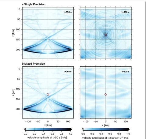
The simulations are performed with a mix of single- and double-floating-point-precision arithmetic. Static parameters such as the medium velocities or density are defined in single precision; however, the FDM calculation and the stress discontinuity at the sources are evaluated more accurately in double precision. We found that sim-ulations in single precision often lead to numerical insta-bility after long-time step calculations, as demonstrated in Fig. 6. The panels in Fig. 6a show snapshots of the par-ticle velocity amplitude in the seismic wavefield obtained by a 2D P-SV numerical simulation using single-precision arithmetic. After a long elapsed time, it was confirmed that a randomly oscillating noise was continuously being radiated from the source location. Such unstable noise is suspected to occur due to the wide dynamic range of the wavefield amplitude near the seismic source, which can-not be handled accurately using single-precision arith-metic. The accumulation of this small error over long time steps may cause problems or instabilities in the simulation. The use of double-precision arithmetic can effectively avoid this problem (Fig. 6b); however, it leads to a considerable increase in the memory usage and com-putation time. OpenSWPC has an option to evaluate all

node (1, 1)

node (2, 1)

node (3, 1)

node (4, 1)

node (nproc_x, 1)

node (1,2

)

node (1,3

)

node (1,4

)

node (1,

npoc_y

)

x _y

z

x

y

a

b

node (1,1

)

nproc_x

nodes nproc_y nodes

MPI data communication s

MPI data communicatio

ns

node (ip, jp) MPI

node (ip+1, jp) node (ip+1,jp+1)

node (ip, jp+1) MPI MPI

MPI

calculations using single-precision arithmetic to reduce the computational cost.

Model input

For the 3D simulation of seismic wave propagation, we consider a layered structure model formed by a set of velocity layers with varying depths. Each layer describes the medium discontinuities with the definitions of medium parameters of density, P- and S-wave velocities, and attenuation (QP,QS) beneath the layer. The depth of

the shallow-most layer corresponds to the topography.

The topography is treated as a staircase boundary with a sufficiently small FDM grid. We assume that z=0 on

the depth axis corresponds to the average sea level; the topography deeper than zero is treated as the seafloor, and the seawater column is filled between the seafloor and z=0.

We adopted NetCDF as the input data format for each layer. The NetCDF format is commonly used in the seismological community, such as in Generic Mapping Tools (GMT; Wessel et al. 2013). In OpenSWPC, a set of NetCDF files and a list of these files associated with the

0

50

100

150

200

z [km

]

−100 −50 0 50 100 x [km]

t=050 s

b Mixed Precision

0.0 0.2 0.4 0.6 0.8 1.0 velocity amplitude at t=50 s [m/s]

−100 −50 0 50 100 x [km]

t=500 s

0.0 0.2 0.4 0.6 0.8 1.0 velocity amplitude at t=500 s [10−4 _m/s] 0

50

100

150

200

z [km]

t=050 s

a Single Precision

t=500 s

medium parameters are used as input to OpenSWPC. Each NetCDF file is defined in geographical coordinates (longitude and latitude) and contains the depth informa-tion at each coordinate locainforma-tion.

Even though the input NetCDF files describe the depths of the boundary at the locations defined by the geograph-ical coordinates, the FDM simulation model needs the depths of the boundary at grids in the Cartesian coordi-nate system. Therefore, a coordicoordi-nate transform is neces-sary to model seismic waves in the Cartesian coordinate system. For this purpose, a coordinate transform based on a power-series expression of the Gauss–Krüger trans-form (Kawase 2011) is embedded in OpenSWPC. Users are requested to input the center of the simulation model in longitude and latitude for the coordinate transform, and the OpenSWPC automatically generates the veloc-ity structure model in the Cartesian coordinate system. Because the grid locations in a Cartesian coordinate sys-tem are usually not identical to the grid locations of the input NetCDF files, a bicubic interpolation is applied to obtain the depth of the boundary.

The layered velocity structure model can be superim-posed by a random velocity fluctuation described by sta-tistical characteristics such as the Gaussian or von Kármán power spectrum density functions (Sato et al. 2012), to sim-ulate the scattering of high-frequency seismic waves in het-erogeneous structures (e.g., Furumura and Kennett 2005; Takemura et al. 2015, 2016). The random velocity pertur-bation is calculated in wavenumber space based on the statistical characteristics of the random medium (Klimeš

2002; Sato et al. 2012). Utility programs to calculate these random velocity fluctuations in 2D and 3D are provided in OpenSWPC. The utility programs provide the random velocity fluctuation data in the NetCDF format, which can be used in OpenSWPC. By customizing the model gen-eration subroutine in OpenSWPC, it is easy to implement another type of velocity model in OpenSWPC if necessary.

Simulation data output

The simulation results are exported as two types of datasets: waveforms at specified station points and 2D snapshots of the seismic wavefield on 2D horizontal and vertical cross sections. For the waveforms, veloc-ity and displacement traces from specified station loca-tions (in either geographical or Cartesian coordinates) are exported in the SAC data format. Because the FDM simulations are performed with much smaller time steps compared to the dominant period of the seismic waves, a temporal decimation is often applied to reduce the data size. The decimation factor is specified in the input parameter file. Note that the integration of velocity waveforms with respect to time to obtain displacement records is performed before the decimation.

The snapshots of the wavefield are stored in NetCDF format files. These cross sections can be taken vertically or horizontally, or along the topography or bathymetry. The snapshots contain the three-component velocity or the displacement motions, or divergence and rotation of the velocity, which are related to the P- and S-waves.

Checkpoint and restart

Most computer systems restrict the maximum com-puter time for a single simulation job via their job queu-ing systems. To cope with this restriction, OpenSWPC is equipped with a checkpoint–restart function that halts the simulation at a specified checkpoint prior to the allowed CPU time and exports all data on memory to files. Then, a new job restarts the simulation from the checkpoint by reading the stored data files of the previ-ous job.

Two‑dimensional codes

OpenSWPC also provides 2D codes for the P-SV and SH models. The 2D FDM simulations use the same input parameter file, except they perform the wave propaga-tion simulapropaga-tions in the x–z plane. A 2D simulapropaga-tion along a cross section of the 3D medium has a much lighter computational load. The horizontal direction of the cross section can be chosen arbitrarily by adjusting the coor-dinate rotation parameter. Note that the 2D codes adopt one-dimensional MPI domain partitioning along the x direction.

Computation performance

Strong‑scale performance measurement

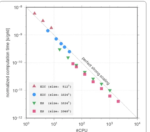
The computational efficiency of the parallel simula-tion was examined using a strong scaling test, where the computation time of a fixed-sized numerical model is measured for parallel computing using different CPU numbers. We performed this test on different computer systems and two different model sizes, a cluster-type computer of the Earthquake Information Center (EIC) system of the Earthquake Research Institute at the Uni-versity of Tokyo with up to 36 Intel Xeon E5-2680 v3 (403.2 GFlops) CPUs, and the Earth Simulator (ES) supercomputer of the Japan Agency for Marine–Earth Science and Technology (JAMSTEC) with up to 2048 the NEC SX-ACE (256 GFlops) CPUs.

The parallel performance was measured for two model sizes: 512×512×512 and 1024×1024×1024 on the

of CPUs for all models. This parallel performance fol-lows a near perfect theoretical scaling, except for cases of over parallelization using very large numbers of CPUs for the small model simulations (e.g., the result of the

1024×1024×1024 model on the ES). This result

sup-ports the efficiency of the parallel simulation of Open-SWPC using a variety of numbers of CPUs from a small (2) to large (2048) number of CPUs.

Figure 8 compares the computational speeds by adopting OpenMP/MPI hybrid computation (hybrid-MPI) relative to pure MPI (flat-MPI) computation. The measurement was taken for the model size of 1024×1024×1024 on

the EIC. A CPU of the EIC has 12 CPU cores. For the flat-MPI parallel computing, the velocity structure model was partitioned and assigned into all cores, and explicit data communications between CPU cores have been made via MPI. On the other hand, the hybrid-MPI computing uti-lizes the shared memory among CPU cores in the CPU, and the MPI data communications were performed only for inter-CPU data exchange. The comparison shows con-siderable improvement in computational performance for the hybrid-MPI, up to 25% speedup compared to the flat-MPI. The speedup ratio slightly increases with increasing numbers of CPUs. These performance improvements in the hybrid programming are in particular because of the efficient reuse of the data on the cache of CPU which are shared among CPU cores (Inoue et al. 2013). We note that the efficiency of the hybrid-MPI may depend on model configurations such as model size or number of CPUs and computer architecture.

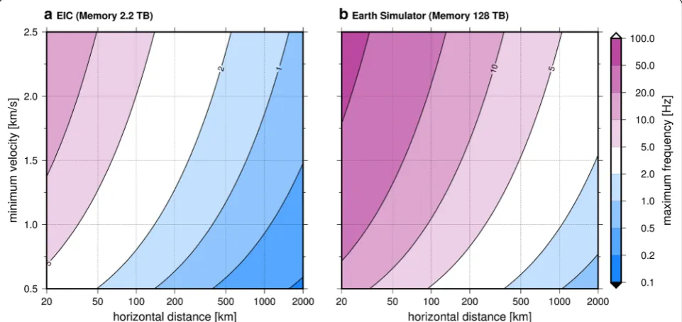
Memory requirements and maximum frequency of the 3D FDM

The maximum size of the 3D FDM simulation and the highest frequency of the seismic waves in the model are bounded by the size of the computer memory. To con-sider the maximum frequency of the simulation, suppose a simulation model has a square horizontal surface with an area of S and a depth of D. OpenSWPC requires a memory of mg =188 bytes per grid when using mixed-precision arithmetic calculations. Discretizing the 3D computational volume with a uniform grid spacing of h indicates that OpenSWPC requires a total memory size, MR, of

Further, the spatial grid size h controls the highest fre-quency allowed for the FDM simulation considering the minimum wavespeed, vmin, such that

where we assume that at least seven grid points per mini-mum wavelength are necessary to restrict the numerical dispersion of the FDM calculation within the required level. Combining the above equations (Eqs. 7, 8), the maxi-mum frequency of the 3D FDM, fmax, can be estimated by

the size of the simulation, the minimum wavespeed and the memory size of the computer Mmax such that

(7) MR=

mgSD

h3 .

(8)

fmax= vmin

7h , perfect strong scalin

g

10−12 10−11 10−10 10−9 10−8

normalized computation time [s/grid]

100 ₁₀1 ₁₀2 ₁₀3 ₁₀4

#CPU ES (size: 20483₎

ES (size: 10243₎

EIC (size: 10243₎

EIC (size: 5123₎

Fig. 7 Speedup of the computational time of the 3D simulation code with increasing numbers of CPUs for different model sizes and com-puter systems. The computation time of each model is normalized by the FDM grid numbers (see text for details)

0.2 0.5 1 2

normalized computation time [s/grid]

flat−MPI

hybrid−MPI

6 12 18 24 36

(x 10−9₎

#CPU

We evaluated the maximum frequency for the 3D FDM simulation on the EIC and the ES as a function of hori-zontal distance in the model and minimum wavespeed (Fig. 9). In this evaluation, we assumed a square simulation model in the horizontal directions with a size of √S and a fixed model depth of D=200 km as a typical simulation

model on a regional scale. For example, assuming a mini-mum S-wavespeed of 1.5 km/s, which corresponds to the P-wavespeed in the ocean column, and a horizontal scale of 200  km, OpenSWPC can simulate a high-frequency seismic wavefield up to 2 and 10 Hz using the EIC and the ES, respectively.

Simulation examples

To demonstrate the effectiveness of OpenSWPC, here we show examples of the seismic wave propagation simula-tions performed by OpenSWPC.

Comparison with the wavenumber integration method We first demonstrate the accuracy of the simulation for a laterally homogeneous medium compared to the result of the wavenumber integration method using the FKRPOG code (Saikia 1994), which is distributed along with the TDMT_INVC moment tensor estimation code (Dreger 2003). The wavenumber integration method is often employed as a reference to validate the accuracy of (9)

fmax=

vmin

7

MR

mgSD 1/3

≤ vmin 7

Mmax

mgSD 1/3

. synthetic seismograms in laterally homogeneous layered _{structures. In this experiment, we assumed the layered}

structure model of Kubo et  al. (2002) and a double-couple point source (strike: 70◦_{, dip: 30}◦ _{and rake: −50}◦₎ placed at a depth of 25 km. The FDM simulation was conducted with a model of 1024×1024×1024 grid

points, a grid size of 0.5 km and a time step of 0.025 s. The reference frequency for Q was set to 1 Hz to match the parameter of the wavenumber integration code. Fig-ure 10 compares the vertical-component seismograms along the x direction obtained by the wavenumber inte-gration method and OpenSWPC. The same band-pass filter of 0.01–0.5 Hz was applied to both traces, consid-ering the expected maximum frequency (∼0.89  Hz) of this simulation. There is excellent agreement between the synthetic seismograms of OpenSWPC and those of the wavenumber integration method from short to large distances and in the wide frequency range below ~1  Hz, demonstrating the effectiveness of OpenSWPC for simulations of seismic wave propagation in an elastic medium.

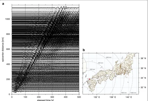
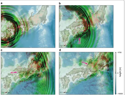
Simulation and visualization with a 3D velocity structure The next example demonstrates the result of a simula-tion of seismic wave propagasimula-tion in a 3D heterogeneous model of the Japan Integrated Velocity Structure Model (JIVSM; Koketsu et al. 2012). The JIVSM consists of a set of sedimentary layers, Conrad and Moho discontinuities, and Pacific and Philippine Sea Plate interfaces associated

with oceanic Mohos and topography. These are rep-resented by the depth variations of each layer and the medium parameters below each depth.

We performed a 3D FDM simulation of the seismic wave propagation for the 2005 West Off Fukuoka Pre-fecture (MW =6.6) earthquake. The source location and the fault mechanism were taken from the F-net moment tensor catalog (Fukuyama et  al. 1998). The simulation model has a spatial grid size of 2000×2560×500 with a

grid spacing of 0.5 km and a time step of 0.025 s with the minimum wavespeed of 1.5  km/s for the shallow-most sedimentary layer. We evaluated the seismic wave propa-gation in the long period band using a source time func-tion with a rise time of 20 s.

The record section of the vertical-component veloc-ity traces (Fig. 11) at the station locations of High Sensi-tivity Seismograph Network Japan (Hi-net) operated by National Research Institute for Earth Science and Disas-ter Resilience (Okada et al. 2004) shows very complicated waves as a result of propagation in the heterogeneous structure. In particular, there are significant wave pack-ets after the arrival of dispersive surface waves at epicen-tral distances over 500 km that seem to be incoherent in neighboring stations. The development of this peculiar

wave packet is clearly seen in the snapshots of the seis-mic wave propagation shown in Fig. 12. It is demonstrated that the direct waves were first radiated from the epicenter and then were trapped in the very low-wavespeed layer of the accretionary prism, which was formed by the subduc-tion of the Philippine Sea Plate (mark A). Then, part of the trapped seismic wave energy was released from the accre-tionary prism and propagated back to the Japanese Archi-pelago (marks B and C), as demonstrated by Furumura et al. (2008) and Guo et al. (2016). As a result, apparently incoherent arrivals appear in the record section (Fig. 11) due to significant off-great-circle propagation.

Note that the visualized seismic wavefield (Fig. 12) was obtained using an associated tool included in the Open-SWPC package. This program reads the wavefield and topography from a NetCDF-formatted output file of the simulation NetCDF file, and the spatiotemporal wave-fields over the topography map are plotted in sequentially numbered portable bitmap files.

Finite‑fault rupture and coseismic deformation

The finite source rupture over the fault is represented in OpenSWPC using multiple sources. To demonstrate this feature, we set up a finite-fault model in a homogeneous 0 10 20 30 40 50 60 70

time [s]

20 40 60 80 100 120 140 160 180 200

distance [km]

half-space as depicted in Fig. 13. A Poisson medium (α/β₌√3) is assumed with an S-wavespeed of

β₌3500  m/s and a density of ρ₌2700  kg/m3 _{. No} attenuation was included in the simulation. We assumed slip with a dip angle of 45◦ _{and a fault size of}

100 km × 50 km. The slip amount is 7.5 m, which cor-responds to a moment magnitude of MW =8.0. In this simulation, the finite-sized fault was represented by 100 × 50 (=5000) point sources along the strike and dip directions, respectively. The moment release was equally distributed over the point sources assuming homogene-ous slip on the fault. The rupture propagation starts from one corner of the fault and spreads over the fault with an assumed constant rupture speed of 2.5 km/s. The source rupture is expressed in OpenSWPC as the delay of the initiation time of each point source. The FDM simula-tion was performed with a 3D model of 600_×600_×400 grid points with a spatial grid size of 0.25 km and time step of 0.01 s.

The simulation result 200  s after the rupture starting time was compared with the analytic solution of Okada

(1985) (Fig. 14). The result of the FDM simulation for the coseismic deformation of the finite-fault source over-all agrees with the analytic solution as demonstrated in previous studies (e.g., Wald and Graves 2001; Maeda and Furumura 2013). Note that the conventional sponge absorbing boundary condition of Cerjan et  al. (1985) leads to an inaccurate estimation of final deformation pattern close to the edge of the fault. In this case, this is most significant in the horizontal dip (y) direction of the fault, and the error grows gradually with increasing time even after the termination of the fault rupture. Con-versely, the estimation using the PML boundary agrees quite well with the analytic solution even if the boundary is very close to the fault.

Plane‑wave incidence

Analysis of regional wave propagation from far-field body waves (Maeda et  al. 2014), core reflected phases (Toya et al. 2017) and the amplification and reflection of seis-mic waves in the shallow structure can be effectively eval-uated by considering the incidence of plane waves. An 0

200 400 600 800 1000

epicenter distance [km]

0 100 200 300 400 500

elapsed time [s]

132˚ E 136˚ E 140˚ E

32˚ N 34˚ N 36˚ N 38˚ N

200 km 400 km

600 km

800 km 1000 km

a

b

example of an FDM simulation for vertical incidences of plane P- and S-waves is shown in Fig. 15. This simulation was performed using the 2D P-SV code with a spatial grid size of 0.2 km and a time step of 0.01 s. The layered veloc-ity structure model of Kubo et  al. (2002) was assumed, and up-going P- and SV-wave packets with characteris-tic wavelengths of 20 km were set near the bottom of the simulation model as initial conditions.

It was found that the use of the PML absorbing bound-ary condition is essential for FDM simulations with inci-dent plane waves as well as with coseismic deformation. With the use of the conventional sponge absorbing bound-ary, artificial reflections from the edge of the model at both sides of the plane wave make it difficult to recognize later arrivals of reflected and converted phases (Fig. 15a). Such

a

b

c

d

(C) (A)

(B)

−10000 0 4700

height [m

]

Fig. 12 Example of a visualization of a seismic wave propagation simulation by OpenSWPC at the elapsed times of a 100 s, b 200 s, c 300 s and d 400 s. Superimposed on the topography map (color scale is shown in the right), scaled absolute amplitude of vertical- and horizontal-component ground velocity motions on the ground surface are shown in red and green, respectively. An additional file contains a time-sequential movie of the seismic wave propagation (Additional file 1)

0 50 100 150

y [k m]

0 50 10

0 150

x [km]

−8

0−

60

−4

0−

20

0

z [km]

artificial reflections are inevitable for plane-wave inci-dence because the attenuation of up-going plane waves in the absorbing boundary leads to artificial diffraction

propagating out of the computational domain, and a part of this packet reflects back inside the model. The situa-tion is much worse for S-wave incidence (Fig. 15b) due 0

50 100 150

0 50 100 150

a Analytic Solution

ux

0 50 100 150

uy

0 50 100 150

uz

0 50 100 150

0 50 100 150

b

ux

0 50 100 150

uy

0 50 100 150

uz

0 50 100 150

0 50 100 150

−1.5 −1.0 −0.5 0.0 0.5 1.0 1.5 u_x [m]

c Sponge

u_x

0 50 100 150

−1.5 −1.0 −0.5 0.0 0.5 1.0 1.5 u_y [m]

u_y

0 50 100 150

−4 −2 0 2 4

u_z [m] u_z

to strong S-to-P conversion at the boundary. Because the PML boundary condition does not modify seismic waves propagating parallel to the boundary, it minimizes the occurrence of such artificial reflections (Fig. 15c, d).

Simulations using the reciprocity theorem

An example of a reciprocity calculation comparing an ordinary forward simulation from the source to receiver and a simulation using the reciprocity theorem with

a P−wave Sponge

0

10

20

30

40

time [s]

0 25 50 75 100

x [km]

b S−wave Sponge

0

10

20

30

40

time [s]

0 25 50 75 100

x [km]

d S−wave PML

0 25 50 75 100

x [km]

c P−wave PML

0 25 50 75 100

x [km]

exchanged source and receiver is shown in Fig. 16. In this simulation, we adopted the JIVSM model (Koketsu et  al. 2012) in northeastern Japan including the topog-raphy variation and seawater column and calculated the seismic waveforms at a F-net station location (N.KSNF) from a source on the Pacific Plate boundary. Both sim-ulations were performed with the same model size of

3000×2400×600 grid points with a discretization of

0.25 km in space and 0.01 s in time. The seismic source is assumed to have a finite source duration time of 4 s.

Figure  16 compares the two simulations without applying a filter. They show excellent agreement with very small residual amplitudes between the two results. Note that the reciprocity theorem (Aki and Richards

2002) assures the exchange of the source and receiver positions only if the absorbing and free surface bound-ary conditions are satisfied (Eisner and Clayton 2001). Therefore, the good agreement between the two simula-tions demonstrates the effectiveness of the free surface and the absorbing boundary conditions in the FDM simulation.

Conclusions and future perspectives

This newly developed FDM simulation code for mod-eling of seismic wave propagation in heterogeneous vis-coelastic media in 2D and 3D, OpenSWPC, has wide applicability for seismological studies and great port-ability, allowing excellent performance from PC clusters to supercomputers. OpenSWPC was designed to apply various models from small to regional scales with the use of various seismic source representations and veloc-ity models. Note that all examples presented in this study were obtained by setting necessary parameters and veloc-ity model files without modifying the simulation code itself. Using OpenSWPC, we can simulate seismic waves at regional scales of up to approximately 1 Hz using PC clusters and up to approximately 10 Hz using high-per-formance supercomputers. All the codes are available with detailed documents at a public repository with an open-source (MIT) license.

In OpenSWPC, we implemented a frequency-inde-pendent attenuation model by adopting the GZB. The assumption of frequency-independent attenuation is Mxx

x−comp

a

10−12 _m

Myy 10−12 m

Mzz 10−12 _m

Myz 10−12 m

Mxz 10−12 m

0 20 40 60 80 100 time [s]

Mxy

0 20 40 60 80 100 time [s]

0 20 40 60 80 100 time [s]

10−12 _m

138˚E 140˚E 142˚E 144˚E 37˚N

38˚N 39˚N 40˚N 41˚N

100 km N.KSNF

b

valid in the low-frequency regime below ∼1 Hz, at least

to a first-order approximation (e.g., Aki and Richards

2002). However, at frequencies above about 1 Hz, attenu-ation appears to follow a power-law frequency depend-ence (e.g., Carcolé and Sato 2010; Phillips et  al. 2014). Incorporation of such different frequency-dependent attenuation properties for high frequencies can also be modeled by applying the memory variable approach (Withers et al. 2015). Such implementation of more real-istic attenuation characterreal-istics to OpenSWPC is a pros-pect for future development.

The OpenSWPC adopts the Cartesian coordinate sys-tem to mainly apply to small-to-regional-scale seismic wave modeling. Recently, Takenaka et al. (2017) proposed a method to incorporate the effect of spherical geometry of the Earth into FDM simulation model in the Cartesian coordinate system. Incorporation of such technique may lead wider applications of OpenSWPC in global seismology without significant modification of present set of the code.

Abbreviations

FDM: Finite Difference Method; EIC: Earthquake Information Center; ES: Earth Simulator; F-net: Full-range seismograph network; GZB: Generalized Zener Body; HOT: Heterogeneity, Oceanic layer and Topography; JIVSM: Japan Integrated Velocity Structure Model; MPI: Message Passing Interface; NetCDF: Network Common Data Form; PML: Perfectly Matched Layer.

Authors’ contributions

TM developed the code based on the original version of the software devel-oped by TF performed simulations with ST, and drafted the manuscript. ST contributed to the design and application of the numerical tests of the code. TF conceived the study and participated in the conception and design of the study. All authors participated in discussions and equally contributed to revising the draft of the manuscript. All authors read and approved the final manuscript.

Author details

1 _{Earthquake Research Institute, The University of Tokyo, 1-1-1 Yayoi,} Bun-kyo 113-0032, ToBun-kyo, Japan. 2 _{National Research Institute for Earth Science} and Disaster Resilience, 3-1 Tennodai, Tsukuba 305-0006, Ibaraki, Japan.

Acknowledgements

We appreciate Phil Cummins, the editor, and two anonymous reviewers for their constructive comments that greatly improved the manuscript. This study was supported by a Collaborative Research Program of the Earthquake Research Institute at the University of Tokyo (2015-B-01). TM was partly sup-ported by the Core-to-Core Collaborative Research Program of the Earthquake Research Institute at the University of Tokyo and the Disaster Prevention Research Institute at Kyoto University (2016-K-06). We used the F-net moment tensor catalog and station location information of the National Research Additional files

Additional file 1. A time-sequential movie of the seismic wave propaga-tion associated with Fig. 12. (6570 KB).

Additional file 2. A time-sequential movie of the displacement field from a finite-fault rupture with the PML absorbing boundary condition associated with Fig. 14. (81.5 KB).

Additional file 3. A time-sequential movie of the displacement field from a finite-fault rupture with the sponge absorbing boundary condition associated with Fig. 14. (94.7 KB).

Institute for Earth Science and Disaster Resilience. We used computer resources of the EIC system of the Earthquake Research Institute at the Uni-versity of Tokyo and the Earth Simulator of the Japan Agency for Marine–Earth Science and Technology.

Competing interests

The authors declare that they have no competing interests.

Availability of data and materials Project name: OpenSWPC

Project home page: http://github.com/takuto-maeda/OpenSWPC Archived version: Version 3.7

https://github.com/takuto-maeda/OpenSWPC/releases Operating system: platform independent

Programing language: Fortran2003 with message passing interface Other requirements: NetCDF library (http://www.unidata.ucar.edu/netcdf) License: MIT license

Any restriction to use by non-academics: None.

Publisher’s Note

Springer Nature remains neutral with regard to jurisdictional claims in pub-lished maps and institutional affiliations.

Received: 27 February 2017 Accepted: 14 July 2017

References

Adams JC, Brainerd WS, Hendrickson RA, Maine RE, Martin JT, Smith BT (2008) The Fortran 2003 Handbook, the complete syntax, features and proce-dures. Springer, London. doi:10.1007/978-1-84628-746-6

Aki K, Richards PG (2002) Quantitative seismology, 2nd edn. University Science Books, Sausalito

Aoi S, Fujiwara H (1999) 3D finite-difference method using discontinuous grids. Bull Seismol Soc Am 89:918–930

Aoi S, Hayakawa T, Fujiwara H (2004) Ground motion simulator: GMS. Butsuri Tansa 57:651–666 (in Japanese with English abstract)

Blanch JO, Robertsson JOA, Symes WW (1995) Modeling of a constant Q: methodology and algorithm for an efficient and optimally inexpensive viscoelastic technique. Geophysics 60:176–184. doi:10.1190/1.1443744 Bohlen T (2002) Parallel 3-D viscoelastic finite difference seismic modelling.

Comput Geosci 28:887–899. doi:10.1016/S0098-3004(02)00006-7 Cao D, Yin X (2014) Equivalence relations of generalized rheological models for

viscoelastic seismic-wave modeling. Bull Seismol Soc Am 104:260–268. doi:10.1785/0120130158

Carcolé E, Sato H (2010) Spatial distribution of scattering loss and intrinsic absorption of short-period S waves in the lithosphere of Japan on the basis of the Multiple Lapse Time Window Analysis of Hi-net data. Geo-phys J Int 180:268–290. doi:10.1111/j.1365-246X.2009.04394.x Cerjan C, Kosloff D, Kosloff R, Reshef M (1985) A nonreflecting boundary

condition for discrete acoustic and elastic wave equations. Geophysics 50:705–708. doi:10.1190/1.1441945

Chen P, Lee EJ (2015) Full-3D seismic waveform inversion. Springer, Cham. doi:10.1007/978-3-319-16604-9

Chew WC, Liu QH (2011) Perfectly matched layers for elastodynamics: a new absorbing boundary condition. J Comput Acoust 04:341–359. doi:10.1142/S0218396X96000118

Coutant O, Virieux J, Zollo A (1995) Numerical source implementation in a 2D finite difference scheme for wave propagation. Bull Seismol Soc Am 85:1507–1512

Cui Y, Poyraz E, Olsen KB, Zhou J, Withers K, Callaghan S, Larkin J, Guest C, Choi D, Chourasia A, Shi Z, Day SM, Maechling JP, Jordan TH (2013) Physics-based seismic hazard analysis on petascale heterogeneous supercomputers. In: Proceedings of SC13 70. doi:10.1145/2503210.2503300

Eisner L, Clayton RW (2001) A reciprocity method for multiple-source simula-tions. Bull Seismol Soc Am 91:553–560. doi:10.1785/0120000222 Emmerich H, Korn M (1987) Incorporation of attenuation into time-domain

computations of seismic wave fields. Geophysics 52:1252–1264. doi:10.1190/1.1442386

Emoto K, Sato G, Nishimura T (2010) Synthesis of vector wave envelopes on the free surface of a random medium for the vertical incidence of a plane wavelet based on the Markov approximation. J Geophys Res 115:B08306. doi:10.1029/2009JB006955

Frankel A, Clayton RW (1986) Finite difference simulations of seismic scatter-ing: implications for the propagation of short-period seismic waves in the crust and models of crustal heterogeneity. J Geophys Res 91:6465–6489. doi:10.1029/JB091iB06p06465

Fukuyama E, Ishida M, Dreger DS, Kawai H (1998) Automated seismic moment tensor determination by using on-line broadband seismic waveforms. Zisin2 51:149–156 (in Japanese with English Abstract)

Furumura T, Chen L (2005) Parallel simulation of strong ground motions during recent and historical damaging earthquakes in Tokyo, Japan. Parallel Comput 31:149–165. doi:10.1016/j.parco.2005.02.003

Furumura T, Kennett BLN (2005) Subduction zone guided waves and the heterogeneity structure of the subducted plate: Intensity anoma-lies in northern Japan. J Geophys Res 110:B10302. doi:10.1029/200 4JB003486

Furumura T, Hayakawa T, Nakamura M, Koketsu K, Baba T (2008) Development of long-period ground motions from the Nankai Trough, Japan, earth-quakes: observations and computer simulation of the 1944 Tonankai (Mw 8.1) and the 2004 SE Off-Kii Peninsula (Mw 7.4) earthquakes. Pure Appl Geophys 165:585–607. doi:10.1007/s00024-008-0318-8

Goldstein P, Dodge D, Firpo M, Minner L (2003) SAC2000: signal processing and analysis tools for seismologists and engineers. In: Lee WHK, Kanamori H, Jennings PC, Kisslinger C (eds) The IASPEI international handbook of earthquake and engineering seismology. Academic Press, London Graves RW (1996) Simulating seismic wave propagation in 3D elastic

media using staggered-grid finite differences. Bull Seismol Soc Am. 86:1091–1106

Graves RW, Wald DJ (2001) Resolution analysis of finite fault source inversion using one- and three-dimensional Green’s functions: 1. Strong motions. J Geophys Res 106:8745–8766. doi:10.1029/2000JB900436

Graves R, Jordan TH, Callaghan S, Deelman E, Field E, Juve G, Kesselman C, Maechling P, Mehta G, Milner K, Okaya D, Small P, Vahi K (2010) Cyber-shake: a physics-based seismic hazard model for southern California. Pure Appl Geophys 168:367–381. doi:10.1007/s00024-010-0161-6

Guo Y, Koketsu K, Miyake H (2016) Propagation mechanism of long-period ground motions for offshore earthquakes along the Nankai Trough: effects of the accretionary wedge. Bull Seismol Soc Am 106:1176–1197. doi:10.1785/0120150315

Helffrich G, Wookey J, Bastow I (2013) The Seismic Analysis Code—a primer and user’s guide. Cambridge University Press, Cambridge. doi:10.1017/ CBO9781139547260

Herrmann RB (1979) SH-wave generation by dislocation sources—a numerical study. Bull Seismol Soc Am 69:1–15

Hsieh MC, Zhao L, Ji C, Ma K-F (2016) Efficient inversions for earthquake slip distributions in 3D structures. Seismol Res Lett 87:1342–1354. doi:10.1785/0220160050

Igel H (2016) Computational seismology: a practical introduction. Oxford University Press, Oxford

Imperatori W, Gallovič F (2017) Validation of 3D velocity models using earth-quakes with shallow slip: case study of the 2014 Mw 6.0 South Napa, California, event. Bull Seismol Soc Am 107. doi:10.1785/0120160041 Inoue S, Tsutsumi S, Maeda T, Minami K (2013) Performance optimization of

seismic wave simulation code on the K computer. IPSJ Trans Adv Comput Syst 6:22–30 (in Japanese with English abstract)

JafarGandomi A, Takenaka H (2007) Efficient FDTD algorithm for plane-wave simulation for vertically heterogeneous attenuative media. Geophysics 72:H43–H53. doi:10.1190/1.2732555

Kawase K (2011) A general formula for calculating meridian arc length and its application to coordinate conversion in the Gauss–Krüger projection. Bull Geosp Inf Auth Jpn 59:1–13

Klimeš L (2002) Correlation functions of random media. Pure Appl Geophys 159:1811–1831. doi:10.1007/s00024-002-8710-2

Koketsu K, Miyake H, Suzuki H (2012) Japan integrated velocity structure model version 1. In: Proceedings of 15th WCEE:1773

Kristek J, Moczo P, Galis M (2009) A brief summary of some PML formulations and discretizations for the velocity-stress equation of seismic motion. Stud Geophys Geodaet 53:459–474. doi:10.1007/s11200-009-0034-6 Kubo A, Fukuyama E, Kawai H, Nonomura K (2002) NIED seismic moment

tensor catalogue for regional earthquakes around Japan: qual-ity test and application. Tectonophysics 356:23–48. doi:10.1016/ S0040-1951(02)00375-X

Lee S-J, Ma K-F, Chen H-W (2006) Three-dimensional dense strong motion waveform inversion for the rupture process of the 1999 Chi-Chi, Taiwan, earthquake. J Geophys Res 111:B11308. doi:10.1029/2005JB004097 Levander AR (1988) Fourth-order finite-difference P-SV seismograms.

Geo-physics 53:1425–1436. doi:10.1190/1.1442422

Madariaga R (1976) Dynamics of an expanding circular fault. Bull Seismol Soc Am 66:639–666

Maeda T, Furumura T (2013) FDM Simulation of seismic waves, ocean acoustic waves, and tsunamis based on tsunami-coupled equations of motion. Pure Appl Geophys 170:109–127. doi:10.1007/s00024-011-0430-z Maeda T, Furumura T, Noguchi S, Takemura S, Sakai S, Shinohara M, Iwai K,

Lee S-J (2013) Seismic- and tsunami-wave propagation of the 2011 Off the Pacific Coast of Tohoku Earthquake as inferred from the tsunami-coupled finite-difference simulation. Bull Seismol Soc Am 103:1456–1472. doi:10.1785/0120120118

Maeda T, Furumura T, Obara K (2014) Scattering of teleseismic P-waves by the Japan Trench: a significant effect of reverberation in the seawater col-umn. Earth Planet Sci Lett 397:101–110. doi:10.1016/j.epsl.2014.04.037 Maeda T, Iwaki A, Morikawa N, Aoi S, Fujiwara H (2016) Seismic-hazard analysis

of long-period ground motion of megathrust earthquakes in the Nankai Trough based on 3d finite-difference simulation. Seismol Res Lett 87:1265–1273. doi:10.1785/0220160093

Mavroeidis GP, Papageorgiou AS (2003) A mathematical representation of near-fault ground motions. Bull Seismol Soc Am 93:1099–1131. doi:10.1785/0120020100

Moczo P (2002) 3D Heterogeneous staggered-grid finite-difference modeling of seismic motion with volume harmonic and arithmetic averaging of elastic moduli and densities. Bull Seismol Soc Am 92:3042–3066. doi:10.1785/0120010167

Moczo P, Kristek J (2005) On the rheological models used for time-domain methods of seismic wave propagation. Geophys Res Lett 32:L01306. doi:1 0.1029/2004GL021598

Moczo P, Kristek J, Galis M (2014) The finite-difference modelling of earth-quake motions. Cambridge University Press, Cambridge. doi:10.1017/ CBO9781139236911

Nakamura T, Takenaka H, Okamoto T, Kaneda Y (2012) FDM simulation of seismic-wave propagation for an aftershock of the 2009 Suruga bay earthquake: effects of ocean-bottom topography and seawater layer. Bull Seismol Soc Am 102:2420–2435. doi:10.1785/0120110356

Nakamura T, Takenaka H, Okamoto T, Ohori M, Tsuboi S (2015) Long-period ocean-bottom motions in the source areas of large subduction earth-quakes. Sci Rep 5:16648. doi:10.1038/srep16648

Noguchi S, Maeda T, Furumura T (2016) Ocean-influenced Rayleigh waves from outer-rise earthquakes and their effects on durations of long-period ground motion. Geophys J Int 205:1099–1107. doi:10.1093/gji/ggw074 Ohminato T, Chouet BA (1997) A free-surface boundary condition for includ-ing 3D topography in the finite-difference method. Bull Seismol Soc Am 87:494–515

Ohminato T, Chouet BA, Dawson P, Kedar S (1998) Waveform inversion of very long period impulsive signals associated with magmatic injec-tion beneath Kilauea volcano. Hawaii. J Geophys Res 103:23839–23862. doi:10.1029/98JB01122

Okada Y (1985) Surface deformation due to shear and tensile faults in a half-space. Bull Seismol Soc Am 75:1135–1154

Okada Y, Kasahara K, Hori S, Obara K, Sekiguchi S, Fujiwara H, Yamamoto A (2004) Recent progress of seismic observation networks in Japan— Hi-net, F-net, K-NET and KiK-net—. Earth Planets Space 56:xv–xxviii. doi:10.1186/BF03353076

Olsen KB, Pechmann JC, Schuster GT (1995) Simulation of 3D elastic wave propagation in the Salt Lake Basin. Bull Seismol Soc Am 85:1688–1710 Petersson NA, Sjogreen B (2014) SW4 user’s guide. Lawrence Livermore

National Laboratory technical report LLNL-SM-662014. https://geody-namics.org/cig/software/github/sw4/v1.1/SW4-v1.1-UsersGuide.pdf. Last accessed June 2017

Petukhin A, Miyakoshi K, Tsurugi M, Kawase H, Kamae K (2016) Visualiza-tion of Green’s funcVisualiza-tion anomalies for megathrust source in Nankai Trough by reciprocity method. Earth Planets Space 68:4. doi:10.1186/ s40623-016-0385-5

Phillips WS, Mayeda KM, Malagnini L (2014) How to invert multi-band, regional phase amplitudes for 2-D attenuation and source parameters: tests using the USArray. Pure Appl Geophys 171:469–484. doi:10.1007/ s00024-013-0646-1

Pitarka A (1999) 3D Elastic finite-difference modeling of seismic motion using staggered grids with nonuniform spacing. Bull Seismol Soc Am 89:54–68 Rew R, Davis G (1990) NetCDF: an interface for scientific data access. IEEE

Comput Graph Appl 10:76–82. doi:10.1109/38.56302

Robertsson JOA, Blanch JO, Symes WW (1994) Viscoelastic finite-difference modeling. Geophysics 59:1444–1456. doi:10.1190/1.1443701 Saikia CK (1994) Modified frequency-wavenumber algorithm for regional

seismograms using Filon’s quadrature: modelling of Lg waves in eastern North America. Geophys J Int 118:142–158. doi:10.1111/j.1365-246X.1994. tb04680.x

Sato H, Fehler MC, Maeda T (2012) Seismic wave propagation and scat-tering in the heterogeneous Earth, 2nd edn. Springer, Berlin. doi:10.1007/978-3-642-23029-5

Takemura S, Furumura T, Maeda T (2015) Scattering of high-frequency seismic waves caused by irregular surface topography and small-scale velocity inhomogeneity. Geophys J Int 201:459–474. doi:10.1093/gji/ggv038 Takemura S, Maeda T, Furumura T, Obara K (2016) Constraining the source

location of the 30 May 2015 (Mw 7.9) Bonin deep-focus earthquake using seismogram envelopes of high-frequency P waveforms: occurrence of deep-focus earthquake at the bottom of a subducting slab. Geophys Res Lett 43:4297–4302. doi:10.1002/2016GL068437

Takenaka H, Fujii Y (2008) A compact representation of spatio-temporal slip distribution on a rupturing fault. J Seismol 12:281–293. doi:10.1007/ s10950-007-9087-6

Takenaka H, Komatsu M, Toyokuni G, Nakamura T, Okamoto T (2017) Quasi-Cartesian finite-difference computation of seismic wave propagation for a three-dimensional sub-global model. Earth Planets Space 69:67. doi:10.1186/s40623-017-0651-1

Tape C, Liu Q, Maggi A, Tromp J (2009) Adjoint tomography of the southern California crust. Science 325:988–992. doi:10.1126/science.1175298 Todoriki M, Furumura T, Maeda T (2017) Effects of sea water on elongated

duration of ground motion as well as variation in its amplitude for off-shore earthquakes. Geophys J Int 208:226–233. doi:10.1093/gji/ggw388 Toya M, Kato A, Maeda T, Obara K, Takeda T, Yamaoka K (2017) Down-dip

variations in a subducting low-velocity zone linked to episodic tremor and slip: a new constraint from ScSp waves. Sci Rep 7:2868. doi:10.1038/ s41598-017-03048-6

Wald DJ, Graves RW (2001) Resolution analysis of finite fault source inver-sion using one- and three-dimeninver-sional Green’s functions: 2. Combining seismic and geodetic data. J Geophys Res 106:8767–8788. doi:10.1029/2 000JB900435

Wessel P, Smith WHF, Scharroo R, Luis J, Wobbe F (2013) Generic Mapping Tools: improved version released. EOS Trans AGU 94:409–410. doi:10.100 2/2013EO450001

Withers KB, Olsen KB, Day SM (2015) Memory-efficient simulation of frequency-dependent Q. Bull Seismol Soc Am 105:3129–3142. doi:10.1785/0120150020

Yoshimitsu N, Furumura T, Maeda T (2016) Geometric effect on a laboratory-scale wavefield inferred from a three-dimensional numerical simulation. J Appl Geophys 132:184–192. doi:10.1016/j.jappgeo.2016.07.002 Zhang W, Shen Y (2010) Unsplit complex frequency-shifted PML

implementa-tion using auxiliary differential equaimplementa-tions for seismic wave modeling. Geophysics 75:T141–T154. doi:10.1190/1.3463431