Time evolution of the fluid flow at the top of the core.
Geomagnetic jerks
Minh Le Huy1,2, Mioara Mandea1, Jean-Louis Le Mou¨el1, and Alexandra Pais1
1Institut de Physique du Globe de Paris, B.P. 89, 4 Place Jussieu, 75252 Paris cedex 5, France 2Hanoi Institute of Geophysics, Nghia do - Tu Liem - Hanoi - Vietnam
(Received August 30, 1999; Revised November 15, 1999; Accepted November 15, 1999)
The knowledge of the geomagnetic field and its secular variation allows us to compute the fluid flow at the core surface. The poloidal and toroidal components of the fluid flow at the core-mantle boundary (CMB) have been calculated every year from the Bloxham and Jackson model (1992) and plotted at 50 year intervals over the last three centuries. The flow patterns conserve some broad features over this whole time-span. The time constant of the degree 1 component of the motion is larger than the time constant of the rest of the flow. The average motion over 300 years appears to be in large part symmetrical with respect to the equator. This average flow can be represented by the sum of a few geostrophic vectors. The acceleration fields corresponding to the well documented jerks of 1969, 1979, 1992 have also been computed. The geometry of these acceleration fields is the same, within a change of sign, for the three events. Moreover, this geometry has close connections with the geometry of the flow itself. The spatial and temporal variations of the flow field can be simply described, in a first approximation; it is possible to give an analytical schematic representation of the flow field during the last three decades. Some characteristics of the decadal length-of-day variations follow if the coupling torque between core and mantle is topographic.
1.
Introduction
The last 20 years (since MAGSAT) have seen spectacu-lar advances in our ability to generate realistic maps of the Earth’s magnetic field outside the planet and at the interface between the fluid core and the overlying solid mantle, us-ing data collected at or above the Earth’s surface. Studies of the field over the last 300 years have revealed some re-markably stable features in the morphology of the field, and it has been discussed whether these features might even have been stable over palaeomagnetic time-scales. Temporal vari-ations are nevertheless conspicuous in data from the last few hundred years, and these variations have implications for the dynamics of the fluid flow at the core-mantle boundary and the coupling mechanism between the core and mantle.
In this paper we will first rely on maps and graphs to single out simple basic features of the behavior of the geomagnetic field in time and space. We will then infer a simplified an-alytic expression of this time-space behavior and use it to suggest an interpretation of decadal length-of-day variations.
2.
Evaluation of the Main Field Variation
Until recent decades, maps and models of the geomagnetic field were usually established for navigation, rather than for understanding the physical process that generates the Earth’s main magnetic field. First restricted to either long time pe-riods sparsely sampled (Fritsche, 1903; Braginsky, 1972; Benkovaet al., 1974 (BKC hereafter); Barraclough, 1974) or to short periods described with some temporal details (Malin,
Copy right cThe Society of Geomagnetism and Earth, Planetary and Space Sciences (SGEPSS); The Seismological Society of Japan; The Volcanological Society of Japan; The Geodetic Society of Japan; The Japanese Society for Planetary Sciences.
1969; Malin and Clark, 1974), models gained more and more accuracy, involved longer time-spans and were produced in a more and more homogeneous way over the period consid-ered.
The Bloxham and Jackson model (1992) (BJ hereafter) is unquestionably the most complete and homogeneous histori-cal description of the main magnetic field presently available. The spatial dependency of the field is represented by a spher-ical harmonic expansion, and the time dependency by a cubic B-spline basis. The expansion in spherical harmonics of the BJ models is limited to order and degree 14. For the tem-poral cubic B-spline basis the knot points have been chosen every 2.5 years. The model consists of two parts (before and after 1840, a limit imposed by the absence of field intensity measurements before this date). The resulting model covers three centuries (1690–1990).
The corresponding maps of the vertical component of the fieldBr(t)at the CMB from 1690 to 1990 are well-known, in the form of a sequence of snapshots at 50 years intervals (see again Bloxham and Jackson, 1992). In the following we only recall some prominent features of the field at the core mantle boundary (CMB). A remarkable standing feature consists of two pairs of intense flux patches, one located under Artic Canada and south-east of Tierra del Fuego and the other un-der Siberia and south-east of Australia. They have remained largely the same for 300 years (Bloxham and Gubbins, 1985). These two pairs of enhanced positive-negative flux patches have been seen as the signature of convective rolls (Gubbins and Bloxham, 1987). Gubbins and Kelly (1993) and Kelly and Gubbins (1997) argue that the two pairs of patches are still present, although subdued, on maps derived from
Fig. 1. Auto-correlation coefficients for different degrees of the geomag-neticfield models considered in this study (thin lines—BCK model, thick lines—BJ model). Left:n=1 (solid line),n=2 (dotted line),n=3 (dashed line) andn= 4 (dot-dashed line). Right: n =5 (solid line),
n=6 (dotted line),n=7 (dashed line) andn=8 (dot-dashed line).
magnetic data averaged over one million years. But Carlut and Courtillot (1995, 1998) claimed that no significant non-zonal term exists in the models derived from palaeomagnetic data. Hulot and Le Mouel (1994) concluded from a study of¨ BJ model that, while the characteristic time constant of the non-dipole terms of thefield model is not larger than some 200 years, the probability of features remaining stationary for a few hundreds years is not negligible.
The Hulot and Le Mouel (1994) analysis considered a three¨ centuries time-span constrained by the BJ models. Using the BKC models, one can go one century further in the past. Let us recall the Hulot and Le Mouel analysis. A quantitative¨ estimate of the stability of the different harmonics(n)can be obtained by computing the correlation function:
Kngh(τ)
used to calculate the current correlation function for a given delayτ; T is the considered time interval (i.e., 300 yr for the BJ models and 400 yr for the BCK models) andδt is the time-step of the geomagnetic models (δt= 1 year here);
gm
n,hmn are the Gauss coefficients.
Figure 1 illustrates the results. K1gh(τ)keeps close to 1 for both models, varying by less than 1 % over four centuries. The decreasing trend for degreesn = 2 andn >5 is
con-firmed. Also, the tendency ofK3gh(τ)andK4gh(τ)to remain stable and larger than 0.5 after 200 years is clear. The prob-ability that such a behavior is compatible with the statistical model of Hulot and Le Mouel is then weaker than considered¨ by the authors when using a shorter 300 years period. The stability of theflux patches is to be related with this longer correlation time of the degrees 3 and 4 harmonics.
Another outstanding feature of the secular variation over the last three centuries is the regular westward drift, at a rate of about 0.28◦/year, of a negative spot on the map of the time derivative (secular variation), B˙r(t), of the vertical component of the field centered on the equator from 1700 (see the BJ models). This does not mean a global westward drift of the secular variationfield; in fact, a westward motion of thefluid at the CMB concentrated in the vicinity of the equator and limited to the western hemisphere was pointed out some time ago (e.g., Gire et al., 1986; Bloxham and Gubbins, 1985).
In the following we will use the vertical component of the magneticfield Br at the CMB, as well as of its secular variationB˙r(t), both provided by the BJ models, from 1690 to 1990. For this time-span we will compute and analyse the evolution of theflow at the top of the core.
3.
Computation of the Flow at the CMB
Wefirst present the evolution of theflow at the CMB on the long term, from 1690 to the present, then for the three last decades of the present century, with more detail.
3.1 Computation of theflow
We compute the large-scale flow using the frozen-flux and tangentially geostrophic hypothesis (Roberts and Scott, 1965; Le Mou¨el, 1984; Gireet al., 1984; Gire and Le Mouel,¨ 1990), which has been supported by recent computations performed locally at the surface of the CMB (Chulliat and Hulot, 1999):
whereuis the horizontal velocityfield at the surface of the core (of the main stream), ∇Hthe gradient operator reduced to horizontal coordinates, θ the co-latitude, ρ is the core density,0is the Earth’s mean rotation,nthe unit outward
radial vector and ∇pthe pressure gradient.
The velocityfield at the top of the core can be represented as the sum of two terms:
u=c∇HS−cn∧ ∇HT (5)
whereSm(c,s) n andT
m(c,s)
n are elementary poloidal and toroidal vectors (e.g., Backus, 1986):
Snm(c,s)=c∇HYnm(c,s) (7)
Tnm(c,s)= −cn∧ ∇HYnm(c,s) (8)
with
Ynm(c,s)=Pnm(cosθ)(cosmφ,sinmφ) (9) wherePnmare Schmidt normalised associated Legendre func-tions. Thesm(c,s)
n ,t m(c,s)
n are the poloidal and toroidal coef-ficients (inr ad yr−1). But, within the geostrophic
approx-imation, u can also be expanded on a basis of elementary geostrophic vectors (Le Mou¨elet al., 1985; Backus and Le Mouel, 1986):¨
u =c
∞
n=1
tn0Tn0+
n
m=1
(snmcVnmc+snmsVnms)
(10)
where T0
n,V m(c,s)
n are the elementary geostrophic vectors.
u(t)has been computed fromBr(t)andB˙r(t), applying the
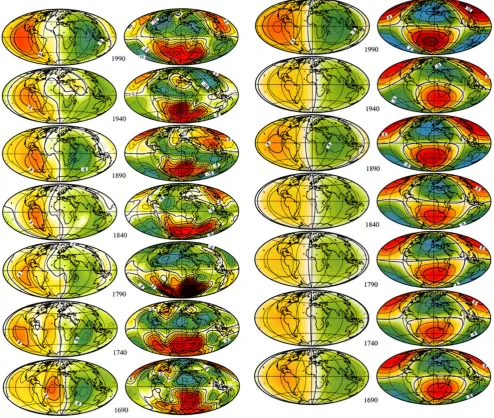
Fig. 2. Poloidal (left) and toroidal (right) scalars,S(t)andT(t), every 50 years. Contour interval: 4·10−4r ad yr−1.
inversion method proposed by Gire and Le Mouel (1990) and¨ discussed by Hulotet al.(1992), with an appropriate choice of parameters. The expansions (6) and (10) are truncated at degree 13.
Figure 2 shows the corresponding maps of the poloidal and toroidal scalars S(t)andT(t)every 50 years. In the following discussion, the zonal toroidal part of theflow is not retained because from our point of view it is partly a secondaryflow accelerated by the pressure torque exerted by the primary non-zonalflow (Jault and Le Mouel, 1990).¨ Afirst simple observation can be readily made: the general organization of theflow tends to conserve some gross fea-tures over the whole considered time-span (the maps suffer of course from large inaccuracies). Let us examine this in more detail. Figure 3 shows the degree 1 component of the poloidal scalar (asinθcos(φ −φ0), wherea is the
ampli-tude of the component of thefirst degree); there is no zonal poloidal component in a geostrophic flow) and the degree 2 component of the toroidal scalar (containingY1
2 andY
2 2
Fig. 4. Auto-correlation coefficients for different degrees of the poloidal (left) and toroidal (right) components of theflow at the CMB:n=1 (solid line),n=2 (dotted line),n=3 (dashed line) andn=4 (dot-dashed line).
harmonics; the zonal toroidal terms will be considered sep-arately for reasons given below). Clearly, the geometry of these components has remained remarkably constant over the period under study (in the case ofY1
1, only the stability
of the origin meridian is of course significant).
As in the case of thefield itself, we have computed the cor-relation function for each degree of the motion. The function
Ks
n is computed for the poloidal part by Eq. (1) wheregmn,
hmn are replaced by snmc, and snms; the function Knt is com-puted for the toroidal part also by Eq. (1) wheregnm,hmn are replaced bytnmc, andtnms. Figure 4 shows the results. Clearly the correlation coefficientsK1s(τ)andK2t(τ)have a behavior different from the others and remain close to 1 for the whole time-span. This means in particular that the geostrophic el-ementary vector:
aV11=a(S11+ηT21) (11)
(ηis a known coefficient; for its expression see Le Mouel¨ et al., 1985; Gire and Le Mouel, 1990), is a stable component¨ of the expansion (10), within a varying amplitudea.
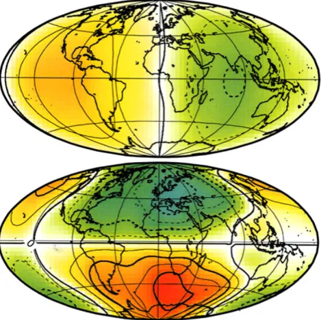
We have also computed the meanflow over the 1690– 1990 time span. Figure 5 shows the average poloidal and toroidal scalars. Clearly S11 andT21 are heavily present in the averageflow; and the flow has a large ingredient sym-metrical with respect to the equator. Figures 6 and 7 repre-sent respectively the equatorially symmetric and equatorially anti-symmetric parts of the poloidal and toroidal scalars (see Hulotet al., 1990) for conventions about the symmetric and anti-symmetric parts of theflow). The symmetric part ofuis quite close toV1
1 (in factV 1s
1 ; the symmetry with respect to
the Greenwich meridian could appear strange; it is not more
Fig. 5. Poloidal (top) and toroidal (bottom) scalars of the motion averaged over three centuries (1690–1990). Contour interval: 4·10−4r ad yr−1.
Fig. 6. Equatorially symmetrical part of the poloidal (top) and toroidal (bottom) scalars of the average motion over three centuries (1690–1990). Contour interval: 4·10−4r ad yr−1.
than for any other meridian). Nevertheless the antisymmet-ric component is not negligible (the energy associated with this component represents about 30 % of the energy of the total averageflow) and contains essentiallyY1
2 andY
2 3 for the
poloidal scalar andY1 1,Y
1 3,Y
2 2,Y
2
4 for the toroidal one. In
Fig. 7. Equatorially anti-symmetrical part of the poloidal (top) and toroidal (bottom) scalars of the motion averaged over three centuries (1690–1990). Contour interval: 4·10−4r ad yr−1.
bV21+dV32=b S21+ζT11+ηT31
+d S32+ζT22+ηT42
. (12)
Figure 8 represents the poloidal and the toroidal scalars corresponding toaV1
1 +bV 1 2 +dV
2
3 (to be compared with
Fig. 5).
To summarize this section, let us say that theflow at the surface of the CMB, taken on average over a few hundreds of years, consists basically of the weighted sum of three elementary geostrophic vectors, one symmetric,V1
1, and the
two other ones antisymmetric, V21 andV32, with respect to the equator. Looking again at Fig. 4, it would be tempting to conjecture thatV1
1 has a longer life time and thatV 1 1 alone
gives, in the main, the average geometry of theflow on larger time spans (larger than a few 102years).
RemarkThe models of thefluidflow at the core surface depend obviously on the quality of the geomagnetic field and secular variation models they are computed from. When using other geomagnetic field and secular variation mod-els (those of Braginsky, 1972; Benkova et al., 1974; and Barraclough, 1974), we find that the morphologies of the correspondingfluidflows, at a given epoch, are quite similar and that the above mentioned characteristics are the same. In fact, the main features of thefluidflow at the CMB can be obtained from secular variation data provided by a distribu-tion of stadistribu-tions as heterogeneous as that of the present-day observatories. For example, using 1959–1986 annual means from 74 observatories, we constructed a secular variation model for every year of the 1960–1985 period in the form of a spherical harmonic expansion up to degree 5 (and degree 1 for the external signal) and derived afluidflow whose mor-phology and energy evolution are the same as for theflow
Fig. 8. Poloidal (top) and toroidal (bottom) scalars of the motion corre-sponding to the sum of three geostrophic vectors,aV1
1,bV 1 2 anddV
2 3.
Contour interval: 4·10−4r ad yr−1.
model derived from the BJfield models (with a much more homogeneous distribution of the observations). This remark underlines the rapid convergence of computations made in the frozen-flux and tangentially geostrophic approximations. In fact, the main features of theflow depend on a small num-ber of parameters (six for the averageflowa,b,dand vector phases; only three if onefixes the symmetry with respect to
φ=0).
4.
The Geomagnetic Jerks and the Behavior of the
Flow during the Last Few Decades
We have considered up to now the evolution of theflow over the whole period where direct observations are available. We will now focus on the last few decades, for which a much finer time sampling is possible. Firstly, we will summarize the methods used to study the so-called geomagnetic jerks. Secondly, we will compare the geometry of successive jerks and the geometry of the velocity flow and the acceleration field, in order to study the relationship between the velocity flow prevailing between the geomagnetic jerks and the ac-celerationfield at the times of these jerks. Finally, we will investigate the space-time variation of theflow at the core-mantle boundary and the consequences on the core-core-mantle coupling and the length-of-day.
4.1 The geomagnetic jerks
Examination of geomagnetic data from worldwide obser-vatories has revealed sudden changes in the trend of the sec-ular variation which have been called“geomagnetic jerks” or“secular variation impulses”and have been discussed by a number of authors (Courtillotet al., 1978; Malin and Hodder, 1982; Malin et al., 1983; Courtillot and Le Mouel, 1984;¨ Kerridge and Barraclough, 1985; McLeod, 1985; Gavoret
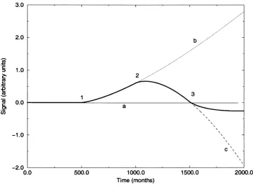
Fig. 9. Thick solid line: Synthetic signal composed of 3 jerks located att0 =(500,1000,1500)with regularitiesα=(1.4,1.6,1.5)and amplitudes
β=(+1.0,−0.75,+1.5). Three lines are extrapolations of the signal obtained by extinguishing successively jerks: the thin solid line (a) is what the signal would have been in the absence of jerks 1, 2, and 3; the dotted line (b) is what the signal would have been if jerks 2 and 3 were absent, and the dashed line (c) is what the signal would have been if jerk 3 was absent.
former analyses established the global character and the in-ternal origin of the jerks. In order to recover more accurate information about these events (time of occurrence, duration, distribution, and other characteristics), we recently applied a wavelet analysis to geomagnetic time series from about one hundred observatories (Alexandrescuet al., 1995, 1996). We found that seven such events took place during the 1900–1990 period, two of which at least (1969 and 1979) could be de-scribed as global in character. A more recent geomagnetic jerk occurring in 1992 has been pointed out by Macmillan (1996) and De Micheliset al. (1998), which has also a world-wide character (Le Huyet al., 1998).
All the events, everywhere, for each component of the geomagneticfield, reveal a singular behavior with a regular-ity close to 1.5. Let us recall what this means. A general expression for the jerk signal is:
j(t|α, β,t0)=βH(t−t0) (t−t0)α, (13)
whereH(t)is the Heaviside distribution,β is an amplitude factor,t0is the starting date of the jerk, andαis its regularity.
The larger the regularity, the smoother the variation of the function. Let us, for illustration, consider a signal f (t)made of 3 jerks:
f (t)= j(t|1.4,1,500)+j(t|1.6,−0.75,1000)
+ j(t|1.5,1.5,1500) . (14)
This signal is shown on Fig. 9. Using wavelet transform allows us to retrieve both the times of the jerks and the reg-ularitiesα (1.4, 1.6, 1.5 in the example); it also gives the amplitudesβ(1.0,−0.75, 1.5) in this synthetic case. In the
case of real data a long series of homogeneous monthly mean values is required to provide good estimates ofβ. Too few series of this kind exist to allow maps of the jerk amplitude (for the three components) to be safely drawn.
So we have used a cruder technique in order to take advan-tage of as many observatories as possible. Let us then recall the technique used by Le Huyet al. (1998). It is considered that in a given time interval [t1,t2], only one geomagnetic
jerk exists at timet0. For a givent0, for each observatory and
for each component (X˙,Y˙,Z˙), two straight-line segments were computed which bestfit the data in the least-squares sense for the time intervals before and aftert0:
˙
E(t)=a1t+b1 t ≤t0
˙
E(t)=a2t+b2 t ≥t0. (15)
The amplitude of the geomagnetic jerkδE¨, for each compo-nent, at each observatory, is defined as the difference between the coefficientsa2anda1. The obtained values are of the
or-der of a fewnT yr−2. The three componentsδX¨,δY¨ and
δZ¨, for the three jerks, are then submitted to a spherical har-monic analysis up to degree 4 (see Le Huyet al., 1998 for details). We checked that the wavelet analysis and Le Huy
et al. techniques provide results in reasonable agreement. Taking the time derivative of Eq. (2) just before and just after the occurrence time of a jerk,t0, and assuming thatBr,
˙
Br (α >1) anduare continuous att =t0:
¨
Br+− ¨Br−= − ∇H. u˙ +− ˙
u−
Br
(16)
i.e.:
Fig. 10. Equatorially symmetrical part of the poloidal (left) and toroidal (right) scalars of the acceleration jumps corresponding to the three jerks (1969, 1979, 1992). Contour interval: 0.4·10−4r ad yr−2.
Fig. 12. a) Degree 2 component of the equatorially symmetric part of the poloidal (left) and toroidal (right) scalars of acceleration jumps cor-responding to the three jerks (1969, 1979, 1992). Contour interval: 0.2·10−4r ad yr−2. b) Degree 2 component of the equatorially
sym-metric part of the poloidal (left) and toroidal (right) scalars of the 1990 flow. Contour interval: 4·10−4r ad yr−1.
where the superscripts“-”and“+”refer to the values before and after the jerk,δB¨r is the radial component of the geo-magnetic jerk at the CMB, andδγis the corresponding jump in the acceleration of thefluidflow at the CMB. The model of Br is again that of Bloxham and Jackson (1992) for the three epochs: 1969, 1979 and 1992 (the model for the latter date is extrapolated from the models of the mainfield and
secular variation for 1990). δB¨ris given by the model ofδB¨
Fig. 11. Equatorially anti-symmetrical part of the poloidal (left) and toroidal (right) scalars of the acceleration jumps corresponding to the three jerks (1969, 1979, 1992). Contour interval: 0.4·10−4r ad yr−2.
Fig. 13. a) Degree 2 component of the equatorially anti-symmetric part of the poloidal (left) and toroidal (right) scalars of acceleration jumps corresponding to the three jerks (1969, 1979, 1992). Contour inter-val: 0.1·10−4r ad yr−2. b) Degree 2 component of the equatorially
anti-symmetric part of the poloidal (left) and toroidal (right) scalars of the 1990flow. Contour interval: 2·10−4r ad yr−1.
computed as described above from (δX¨,δY¨andδZ¨). Brand
Fig. 14. a) Degree 3 component of the equatorially symmetric part of the poloidal (left) and toroidal (right) scalars of acceleration jumps cor-responding to the three jerks (1969, 1979, 1992). Contour interval: 0.2·10−4r ad yr−2. b) Degree 3 component of the equatorially
sym-metric part of the poloidal (left) and toroidal (right) scalars of the 1990 flow. Contour interval: 4·10−4r ad yr−1.
of elementary geostrophic vectors as in Eq. (10).
4.2 Comparison of the geometry of successive jerks
We will focus on the 1969, 1979, 1992 jerks since they are by far the best documented. We have already discussed this comparison in Le Huyet al. (1998); we now elaborate on this and emphasize outstanding features.
Figure 10 shows the equatorially symmetric parts of the poloidal and toroidal scalars corresponding to the three jerks. The geometry is broadly the same for the three jerks, with a change of sign in 1979 compared to 1969 and 1992. Figure 11 is the same for the equatorially anti-symmetric part. The sim-ilarity of the geometries, within the sign change in 1979, is even more striking, especially for the toroidal scalar. Figures 12 (a), 13 (a), 14 (a), 15 (a) show the same pictures separately for the components of degrees 2 and 3 of the poloidal and toroidal scalars, for the three jerks. The similarity of the 1969, 1979 and 1992figures, within a sign change in 1979, is conspicuous (despite some observable phase shifts).
4.3 Comparison of the geometries of the velocityflow and the accelerationfield
Let us now compare the geometry of the flow u deter-mined at a given time—we chose 1990, the last date of the BJ model—with the geometry of the jerks (the same for all three in afirst gross approximation—as described above). For this comparison we retain only the low degree terms (the expansion of ugoes to degree 13, while the expansion of
δγ goes only up to degree 4;δB¨r models, obtained as de-scribed above, are more difficult to get and less accurate than models of secular variation). Figures 12 (b), 13 (b), 14 (b), 15 (b) show the degree 2 and 3 components of the
equatori-Fig. 15. a) Degree 3 component of the equatorially anti-symmetric part of the poloidal (left) and toroidal (right) scalars of acceleration jumps corresponding to the three jerks (1969, 1979, 1992). Contour inter-val: 0.1·10−4r ad yr−2. b) Degree 3 component of the equatorially
anti-symmetric part of the poloidal (left) and toroidal (right) scalars of the 1990flow. Contour interval: 2·10−4r ad yr−1.
ally symmetric part and the equatorially anti-symmetric part of the poloidal scalar of the 1990flowu, to be compared with the samefigures (a).
The components of theflow and of the acceleration jump for the same degrees have similar morphologies. However, there is a distinct shift in longitude (about 40–50◦), between theflow and the acceleration jump, for a given degree.
4.4 Space time variation of theflow at the CMB for the last three decades
1) In previous papers (Alexandrescuet al., 1995, 1996) it was shown that the regularity of the jerks is the same (≈ 3/2) for the three components of thefield, everywhere at the Earth’s surface, both for the 1969 and 1979 events and it seems to be again the same in 1992 (in most observatories the lengths of the geomagnetic series after this date are not long enough to allow a proper analysis of this last jerk by wavelets). It results that each jerk component ofB(θ, φ,t)
(Bx,By,Bz) defined as in Eq. (13) is of the form:
Bi j(θ, φ,t)=bi j(θ, φ)H(t−tj)(t−tj)3/2 (18)
where j= 1969, 1979, 1992,i=x,y,z.
2) The present study shows that the acceleration jump— jerk —is, in afirst approximation, the same for the three eventstj within a sign change. From the remarks 1) and 2) and the form of the induction equation, it results that a simple schematic representation of the velocityfielduat the CMB, from a few years before 1969 up to now is:
u(t, θ, φ)= u0(t, θ, φ)
Fig. 16. Behavior of length-of-day monthly means averaged overfive years (dashed line) and of residuals of a quadratic regression applied to a synthetic signal composed of 3 jerks (see also Fig. 9) located att0=(1969,1979,1992)with the regularitiesα=(1.5,1.5,1.5)and amplitudesβ=(+1.0,−1.0,+1.0) (solid line).
+η2H(t−t2)·(t−t2)1/2
+η3H(t−t3)·(t−t3)1/2]δγ (θ, φ) (19)
where the coefficientsη1, η2, η3, with dimensionL T−3/2are
the amplitudes of thet1,t2,t3jerks in the velocityfield. δγ
(dimensionless) characterises the geometry of the jerk in the velocityu(regularity 1/2).
4.5 Consequences on the core-mantle coupling and length-of-day
From Eq. (3), the pressure p has a similar expression to (19):
p(t, θ, φ)= p0(t, θ, φ)+
η1H(t−t1)·(t−t1)1/2
+η2H(t−t2)·(t−t2)1/2
+η3H(t−t3)·(t−t3)1/2
·δp(θ, φ)ρ0c (20)
whereρis density,0the Earth’s mean rotation andδp(θ, φ)
(dimensionless) characterizes the geometry of the jerk on pressure (regularity 1/2).
Let us suppose that the axial torque exerted on the mantle by the core is essentially a topographic torque (Hide, 1989; Jault and Le Mouel, 1989, 1999; Hide¨ et al., 1993):
(t)= −
C M B
p(t, θ, φ)∂h
∂φ(θ, φ)dS (21)
wherehis the deviation of the CMB from the mean sphere. Whence, due to the fact thath(θ, φ) is constant in time, it comes:
(t)=0(t)+
η1H(t−t1)·(t−t1)1/2+η2H(t−t2)
·(t−t2)1/2+η3H(t−t3)·(t−t3)1/2
1 (22)
with
0(t)= −
C M B
p0(t, θ, φ)
∂h
∂∗φ(θ, φ)dS (23)
1= −ρ0c
C M B
δp(θ, φ)∂h
∂φ(θ, φ)dS. (24)
Now, fromImd/dt=, it comes:
(t)=(t0)+
t
t0
(0(t)/Im)dt+ 2
3
1 Im
η1H(t−t1)(t−t1)3/2+η2H(t−t2)(t−t2)3/2
+η3H(t−t3)(t−t3)3/2
. (25)
The termtt
0(0(t)/Im)dt is actually unknown. It includes
not only the effect of a smoothly changing pressure on a standing topography h(θ, φ), but also the effect of the dis-placement —due to rotation itself—of the pressurefield
p0with respect toh (Jault and Le Mouel, 1991). It has to¨
be supposed, if the topography is as large as given by some seismologists (Morelli and Dziewonski, 1987; Forte et al., 1995), that the value of0 is much smaller than the value
which could be derived from order of magnitude compu-tations; some orthogonality relationship between p0 andh
must be satisfied. Such a relation betweenδp andh is not assumed; there is a quite significant phase shift between the jerk acceleration and theflow (Fig. 12 to 15), and the jerk contribution is smaller (the contribution of thetjjerk is just zero at timetj).
Therefore we just compute a smooth simple trend to rep-resent(t0)+
t
the jerk signal (3rd member of the right hand side of Eq. (25)) gives a good representation of the length-of-day from, say, 1960. The essential point is that the singularities are in the jerk signal; the same regularityαis assumed for each singu-larity. The results are illustrated in Fig. 16. The 1969, 1979, 1992 magnetic events are followed by maxima in, with a lag of a few years (about 3 years). This is to be compared with the features of the real data curve, as was done by Pais
et al., 1999. Note that singularities with regularitiesα=3/2 should be found in length-of-day data at timetj. The present reasoning remains of course qualitative.
5.
Conclusion
We have tried to single outfirst-order gross features of the spatio-temporal behavior of theflow at the CMB computed in the frozen-flux and tangential geostrophic approximations. The geometry as well as the temporal variation look—to this approximation—very simple. Theflow can indeed be represented, for its main part, by the sum of a few geostrophic elementary vectors. Coming to a more accurate description of the last three decades, the geometries of the acceleration flows corresponding to the three jerks of 1969, 1979, 1992 are similar, within a sign change for the 1979 event. Simi-larities also exist between the geometry of the acceleration jumps and theflow itself. The memory of the jerkflows over ten year time intervals is probably not to be attributed to some kind of interaction with the mantle through the CMB. More probably, it is a consequence of the existence of sim-ple standing features of theflow. No physical interpretation has been tempted here. We have also derived an analytical schematic representation of theflowfield for the last three decades which could account for some characteristics of the decade of length-of-day variations. As usual, the inadequacy of the data appears as a main limitation to the analysis. Com-bining simultaneous satellite and observatory data will in the near future help in better understanding these processes.
Acknowledgments. We thank Hisayoshi Shimizu and David
Barraclough for their helpful comments on an earlier version of the manuscript. This is IPGP contribution 1642.
References
Alexandrescu, M., D. Gibert, G. Hulot, J. -L. Le Mou¨el, and G. Saracco, Detection of geomagnetic jerks using wavelet analysis,J. Geophys. Res.,
100(B7), 12557–12572, 1995.
Alexandrescu, M., D. Gibert, G. Hulot, J. -L. Le Mou¨el, and G. Saracco, Worldwide wavelet analysis of geomagnetic jerks,J. Geophys. Res.,
101(B10), 21975–21994, 1996.
Backus, G. E., Poloidal and toroidalfields in geomagneticfield modeling,
Rev. Geophys.,24, 75–109, 1986.
Backus, G. E. and J. -L. Le Mou¨el, The region of the core-mantle boundary where geostrophic velocityfields can be determined from frozen-flux magnetic data,Geophys. J. R. Astron. Soc.,85, 617–628, 1986. Barraclough, D. R., Spherical harmonic analyses of the geomagneticfield
for eight epochs between 1600 and 1910,Geophys. J. R. Astron. Soc.,36, 497–513, 1974.
Benkova, N. P., G. I. Kolomiytseva, and T. N. Cherevko, Analytical model of the geomagneticfield and its secular variation over a period of 400 years (1550–1950),Geomagn. Aeron.,14, 751–755, 1974.
Bloxham, J. and D. Gubbins, The secular variation of Earth’s magneticfield,
Nature,317, 777–781, 1985.
Bloxham, J. and A. Jackson, Time-dependent mapping of the magneticfield at the core-mantle boundary,J. Geophys. Res.,97, 19537–19564, 1992. Braginsky, S. I., Spherical analyses of the main geomagneticfield in 1550–
1800,Geomag. Aeron.,12, 524–529, 1972.
Carlut, J. and V. Courtillot, Geomagnetic paleosecular variation in the last 5 million years: How many multipoles are actually resolvable? (abstract),
EOS Suppl.,76(46), 166 , 1995.
Carlut, J. and V. Courtillot, How complex is the time-averaged geomagnetic field over the past 5 Myr?,Geophys. J. Int,134, 527–544, 1998. Chulliat, A. and G. Hulot, Local computation of the geostrophic pressure at
the top of the core,Phys. Earth Planet. Inter.,117, 309–328, 2000. Courtillot, V. and J. -L. Le Mou¨el, Geomagnetic secular variation impulses,
Nature,311, 709–716, 1984.
Courtillot, V., J. Ducruix, and J. -L. Le Mou¨el, Sur une acc´el´eration r´ecente de la variation s´eculaire du champ magn´etique terrestre,C. R. Acad. Sci. Paris,287, S´erie D., 1095–1098, 1978.
De Michelis, P., L. Cafarella, and A. Meloni, Worldwide character of the 1991 jerk,Geophys. Res. Lett.,25, 377–380, 1998.
Forte, A. M., J. X. Mitrovica, and R. L. Woodward, Seismic-geodynamic de-termination of the origin of excess ellipicity of the core-mantle boundary,
Geophys. Res. Lett.,22(9), 1013–1016, 1995.
Fritsche, H.,Atlas des Erdmagnetismus, pp. 1–26, Riga, 1903.
Gavoret, J., D. Gibert, M. Menvielle, and J. -L. Le Mou¨el, Long-term vari-ations of the external and internal components of the Earth’s magnetic field,J. Geophys. Res.,91(B5), 4787–4796, 1986.
Gire, C. and J. -L. Le Mou¨el, Tangentially geostrophicflow at the core-mantle boundary compatible with the observed geomagnetic secular vari-ation: the large-scale component of theflow,Phys. Earth Planet. Inter.,
59, 259–287, 1990.
Gire, C., J. -L. Le Mou¨el, and J. Ducruix, Evolution of the geomagnetic secular variationfield from the beginning of the century,Nature,307, 349–352, 1984.
Gire, C., J. -L. Le Mou¨el, and T. Madden, Motions at the core surface derived from secular variation data,Geophys. J. R. Astron. Soc.,84, 1–29, 1986. Golovkov, V. P., T. I. Zvereva, and A. O. Simonyan, Common features and differences between“jerks”of 1947, 1958 and 1969,Geophys. Astrophys. Fluid Dyn.,49, 81–96, 1989.
Gubbins, D. and J. Bloxham, Morphology of the geomagneticfield and implications for the geodynamo,Nature,325, 509–511, 1987. Gubbins, D. and L. Tomlinson, Secular variation from monthly means from
Apia and Amberley magnetic observatories,Geophys. J. R. Astron. Soc.,
86, 603–616, 1986.
Gubbins, D. and P. Kelly, Persistent patterns in the geomagneticfield over the past 2.5 Myr,Nature,365, 829–832, 1993.
Hide, R., Fluctuations in the Earth’s rotation and the topography of the core-mantle interface,Phil. Trans. R. Soc. Lond.,A328, 351–363, 1989. Hide, R., R. W. Clayton, B. H. Hager, M. A. Speith, and C. V. Voorhies, Topographic core-mantle coupling andfluctuations in the Earth’s rotation, inRelating Geophysical Structures and Processes: The Jeffreys Volume, edited by K. Aki and R. Dmowska, Geophys. Monog., Amer. Geophys. Un.,76, 107–120, 1993.
Hulot, G. and J. -L. Le Mou¨el, A statistical approach to the Earth’s main magneticfield,Phys. Earth Planet. Inter.,82, 167–183, 1994.
Hulot, G., J. -L. Le Mou¨el, and D. Jault, Theflow at the core-mantle bound-ary: symmetry properties,J. Geomag. Geoelectr.,42, 857–874, 1990. Hulot, G., J. -L. Le Mou¨el, and J. Wahr, Taking into account truncation
problems and geomagnetic model accuracy in assessing computedflows at the core-mantle boundary,Geophys. J. Int.,108, 224–246, 1992. Jault, D. and J. -L. Le Mou¨el, The topographic torque associated with a
tangentially geostrophic motion at the core surface and inferences on the flow inside the core,Geophys. Astrophys. Fluid Dyn.,48, 273–296, 1989. Jault, D. and J. -L. Le Mou¨el, Core mantle boundary shape: constraints inferred from the pressure torque acting between the core and the mantle,
Geophys. J. Int.,101, 233–241, 1990.
Jault, D. and J. -L. Le Mou¨el, Exchange of angular momentum between the core and the mantle,J. Geomag. Geoelectr.,43, 111–129, 1991. Jault, D. and J. -L. Le Mou¨el, Comment on‘On the dynamics of
topograph-ical core-mantle coupling’by Weijia Kuang and Jeremy Bloxham,Phys. Earth Planet. Inter.,114, 211–215, 1999.
Kelly, P. and D. Gubbins, The geomagneticfield over the past 5 million years,Geophys. J. Int.,128, 315–330, 1997.
Kerridge, D. J. and D. R. Barraclough, Evidence for geomagnetic jerks from 1931 to 1971,Phys. Earth Planet. Inter.,39, 228–236, 1985.
Le Mou¨el, J. -L., Outer-core geostrophicflow and secular variation of Earth’s geomagneticfield,Nature,311, 734–735, 1984.
Le Mou¨el, J. -L., C. Gire, and T. Madden, Motions at the core surface in the geostrophic approximation,Phys. Earth Planet. Inter.,39, 270–287, 1985.
characteristics of successive geomagnetic jerks,Earth Planets Space,50, 723–732, 1998.
Macmillan, S., A geomagnetic jerk for the early 1990’s,Earth Planet. Sci. Lett.,137, 189–192, 1996. Malin, S. R. C., Geomagnetic secular varia-tion and its changes, 1942.5 to 1962.5,Geophys. J. R. Astron. Soc.,17, 415–441, 1969.
Malin, S. R. C. and A. D. Clark, Geomagnetic secular variation, 1962.5 to 1967.5,Geophys. J. R. Astron. Soc.,36, 11–20, 1974.
Malin, S. R. C. and B. M. Hodder, Was the 1970 geomagnetic jerk of internal or external origin?,Nature,296, 726–728, 1982.
Malin, S. R. C., B. M. Hodder, and D. R. Barraclough, Geomagnetic secular variation: a jerk in 1970, in75th Anniversary Volume of Ebro Observa-tory, edited by J. O. Card´us, pp. 239–256, Ebro Obs., Tarragona, Spain, 1983.
McLeod, M. G., On the Geomagnetic jerk of 1969,J. Geophys. Res.,90, 4597–4610, 1985.
Morelli, A. and M. Dziewonski, Topography of the core-mantle boundary
and lateral homogeneity of the liquid core,Nature,325, 678–683, 1987. Pais, A., G. Hulot, M. Mandea Alexandrescu, Does the geomagnetic secular variation anticipate or correlate with decade length of day variations? (Abstract), IUGG Birmingham, 1999.
Roberts, P. H. and S. Scott, On the analysis of the secular variation. 1. A hydromagnetic constraint: theory.,J. Geomag. Geoelectr.,17, 137–151, 1965.
Stewart, D. N. and K. Whaler, Geomagnetic disturbancefields: An analysis of observatory monthly means,Geophys. J. Int.,108, 215–223, 1992. Whaler, K. A., A new method for analysing geomagnetic impulses,Phys.
Earth Planet. Inter.,48, 221–240, 1987.