Performance analysis of wavelet transforms and morphological operator based classification of epilepsy risk levels

(1)

R E S E A R C H

Open Access

Performance analysis of wavelet transforms and

morphological operator-based classification of

epilepsy risk levels

Rajaguru Harikumar

*

, Thangavel Vijayakumar

Abstract

The objective of this paper is to compare the performance of singular value decomposition (SVD), expectation maximization (EM), and modified expectation maximization (MEM) as the postclassifiers for classifications of the epilepsy risk levels obtained from extracted features through wavelet transforms and morphological filters from electroencephalogram (EEG) signals. The code converter acts as a level one classifier. The seven features such as energy, variance, positive and negative peaks, spike and sharp waves, events, average duration, and covariance are extracted from EEG signals. Out of which four parameters like positive and negative peaksand spike and sharp waves, events and average duration are extracted using Haar, dB2, dB4, and Sym 8 wavelet transforms with hard and soft thresholding methods. The above said four features are also extracted through morphological filters. Then, the performance of the code converter and classifiers are compared based on the parameters such as performance index (PI) and quality value (QV).The performance index and quality value of code converters are at low value of 33.26% and 12.74, respectively. The highest PI of 98.03% and QV of 23.82 are attained at dB2 wavelet with hard thresholding method for SVD classifier. All the postclassifiers are settled at PI value of more than 90% at QV of 20.

Keywords:EEG signals; Morphological operators; Wavelet transforms; Code converter; Singular value decomposition; Expectation maximization; Modified expectation maximization

1 Introduction

The electroencephalogram (EEG) is a measure of cumu-lative firing of neurons in various parts of the brain [1]. It contains information regarding changes in the elec-trical potential of the brain obtained from a given set of recording electrodes. These data include the characteris-tic waveforms with accompanying variations in ampli-tude, frequency, phase, etc., as well as brief occurrence of electrical patterns such as spindles, sharps, and spike waveforms [2]. EEG patterns have shown to be modified by a wide range of variables including biochemical, metabolic, circulatory, hormonal, neuroelectric, and be-havioral factors in [3]. In the past, the encephalographer, by visual inspection, was able to qualitatively distinguish normal EEG activity from either the localized or gener-alized abnormalities contained within relatively long EEG records [4]. The most important activity possibly

detected from the EEG is the epilepsy [5]. Epilepsy is characterized by an uncontrolled excessive activity or potential discharge by either a part or all of the central nervous system [5]. The different types of epileptic seizures are characterized by different EEG waveform patterns [6]. With real-time monitoring to detect epi-leptic seizures gaining widespread recognition, the advent of computers has made it possible to effectively apply a host of methods to quantify the changes occur-ring based on the EEG signals [4]. The EEG is an im-portant clinical tool for diagnosing, monitoring, and managing neurological disorders related to epilepsy [7]. This disorder is characterized by sudden recurrent and transient disturbances of mental function and/or movements of body that results in excessive discharge group of brain cells [8]. The presence of epileptiform activity in the EEG confirms the diagnosis of epilepsy, which sometimes may be confused with other disor-ders producing similar seizure-like activity [9]. Be-tween seizures, the EEG of a patient with epilepsy may * Correspondence:[email protected]

Bannari Amman Institute of Technology, Sathyamangalam, Tamil Nadu 638401, India

(2)

be characterized by occasional epileptic form transients-spikes and sharp waves [10]. Seizures are featured by short episodic neural synchronous discharges with considerably enlarged amplitude. This uneven synchrony may hap-pen in the brain accordingly, i.e., partial seizures can be visible only in few channels of the EEG signal or generalized seizures, that are seen in every channel of the EEG signal involving the whole brain [11]. Epileptic seizure is an abnormality in EEG gathering and is featured by short and episodic neuronal synchronous discharges with severely high amplitude. This anomal-ous synchrony may happen in the brain locally (partial seizures) and is visible only in fewer channels of the EEG signal or including the entire brain, i.e., visible in all the channels of the EEG signal [12].

1.1 Related works

In the last three decades, the analysis and classification of epilepsy from EEG signal has become a fascinating research. A huge volume of research has already been performed which includes spike detection, classification epilepsy seizures, ictal and inter ictal analysis, nonlinear and linear analysis and soft computing methods. Gotman [9] discussed the improvement of epileptic seizure detec-tion and evaluadetec-tion. Pang et al. [10] summarized the history and evaluation of various spike detecting algorithms. The authors in [13] have discussed the different neural networks as a function approximation and universal approximation for epilepsy diagnosis. Rezasarang [14] encapsulated the performance of spike detecting algorithms in terms of sen-sitivity, specificity, and average detection. Rezasarang [14] orders the performance of spike detecting algorithms in terms of good detection ratio (GDR). McSharry et al. [8] discussed and enumerated the nonlinear methods and its relevance to predict epilepsy by considering EEG samples as time series. Majumdar [15] reviews various soft comput-ing approaches of EEG signals which emphasize more on pattern recognition techniques. The paper [15] mainly fo-cuses on dimensionality reduction, SNR problems, linear and soft computing techniques for EEG signal processing. Majumdar concludes that the neural network and Bayesian approaches are two popular choices even though linear statistical discriminants are easier to implement. Great deals of support vector machines (SVM) are also discussed in this paper for their classification accuracy. Hence, the EEG signal occupies a great deal of data regarding the work of the brain. However, classification and estimation of the signals are inadequate. As there is no explicit category sug-gested by the experts, visual examination of EEG signals in time domain may be deficient. Routine clinical diagnosis necessitates the analysis of EEG signals [13]. Hence, auto-mation and computer methods have been utilized for this reason. Current multicenter clinical analysis indicates con-firmation of premonitory symptoms in 6.2% of 500 patients

with epilepsy [16]. Another interview-based study found that 50% of 562 patients felt‘auras’before seizures. Those clinical data provide a motivation to search for pre-monitoring alterations on EEG recordings from the brain and to employ a device that can act without human inter-vention to forewarn the patient [17]. On the other hand, despite decades of research, existing techniques do not yield to better performance. This paper addresses the ap-plication and comparison of singular value decomposition (SVD), expectation maximization (EM), and modified expectation maximization (MEM) classifiers towards optimization of code converter outputs in the classifi-cation of epilepsy risk levels.

Weber et al. [18] have proposed the three-stage design of an EEG seizure detection system. The first stage of the seizure detector compresses the raw data stream and transforms the data into variables which represent the state of the subject's EEG. These state measures are re-ferred to as context parameters. The second stage of the system is a neural network that transforms the state measures into smaller number of parameters that are intended to represent measures of recognized phenom-ena such as small seizure in the EEG [9,10]. The third stage consists of a few simple rules that confirm the ex-istence of the phenomena under consideration. Similarly, this paper also presents a three-stage design for epilepsy risk level classification. The first stage extracts the seven required distinct features from raw EEG data stream of the patient in time domain. The next stage transforms these features into a code word through a code converter with seven alphabets which represents the patient's state in five distinct risk levels for a 2-s epoch of EEG signal per chan-nel. The last stage is a SVD, EM, or MEM which optimizes the epilepsy risk level of the patient. The organization of the paper is as follows. Section 1 introduces the paper and materials, and its methods are discussed in Section 2. Section 3 describes about the SVD, EM, and MEM as post-classifiers for epilepsy risk level classification. Results are discussed in Section 4, and the paper is concluded in Section 5.

2 Materials and methods

2.1 Data acquisition of EEG signals

(3)

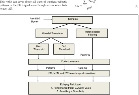
duration. A 2-s epoch is long enough to detect any signifi-cant changes in activity and presence of artifacts and also short enough to avoid any redundancy in the signal [19]. For a patient, there are 16 channels over three epochs. Having a frequency of 50 Hz, each epoch was sampled at a frequency of 200 Hz. Each sample corresponds to the instantaneous amplitude values of the signal, totaling to 400 values for an epoch. Figure 1 shows the model of the flow diagram of epilepsy risk level classification system. Four types of artifacts were present in our data. They included eye blink, electromyography (EMG) artifact, and chewing and motion artifacts [20]. Approximately, 1% of the data was artifacts. We did not make any attempt to select certain number of artifacts and of a specific nature. The objective of including artifacts was to have spikes versus nonspike categories of waveforms. The latter could be a normal background EEG and/or artifacts [21]. In order to train and test the feature extractor and classifiers, we need to select a suitable segment of EEG data. In our experiment, the training and testing were selected through a short sampling window and all EEG signals were visually examined by a qualified EEG technologist. A neurologist's decision regarding EEG features (or normal EEG segment) was used as the gold standard. We choose a sample window of 400 points corresponding to 2 s of the EEG data. This width can cover almost all types of transient epileptic patterns in the EEG signal, even though seizure often lasts longer [22].

In order to classify the risk level of the patients, certain parameters were chosen which are detailed below:

1. For every epoch, the energy is calculated as [4]

E¼X

n

i¼1

x2i ð1Þ

where xiis the signal sample value and n is the number

of such samples.

2. One of the simplest linear statistics that may be used for investigating the dynamics of underlying the EEG is the variance of the signal calculated in consecutive nonoverlapping windows. The variance (σ) is given by

σ2_¼

Xn i¼1 xi

−μ

ð Þ2

n ð2Þ

whereμis the average amplitude of the epoch.

3. For the average variance, the covariance of duration is determined by using the equation below:

CD¼

Xp i¼1

D−ti

ð Þ2

pD2 ð3Þ

EM, MEM and SVD used as post classifiers

Epilepsy Risk Level 1. Performance Index 2.Quality value

3. Sensitivity 4.Specificity Code converters

Samples Raw EEG

Signals

Patterns Patterns

Morphological Filtering

Soft Threshold Wavelet Transform

Features Hard

Threshold

(4)

The following are the four parameters which are ex-tracted using morphological filters and wavelet transforms:

1. The total number of positive and negative peaks is found above the threshold.

2. For a zero crossing function, if it lies between 20to 70 ms, then the spikes can be detected. If the zero crossing function lies between 70to 200 ms then the sharp waves are detected when the zero crossing function lies between 70 to 200 ms.

3. After having detected, the total number of spikes and sharp waves were determined as the events. 4. The duration for these waves is determined by the

relation:

D¼

Xp i¼1

ti

p ð4Þ

wheretiis the peak to peak duration and pis the

num-ber of such durations.

2.2 Wavelet transforms for feature extraction

The brain signals are nonstationary in nature. In order to capture the transients and events of the waveforms, we are in dire state to visualize the time and frequency simultaneously. Hence, the wavelet transforms are the better choice to extract the transient features and events from the EEG signals. The wavelet transform-based fea-ture extraction is discussed as follows:

Let us consider a functionf(t). The wavelet transform of this function is defined as [23]

wf að ;bÞ ¼

Z∞

−∞

f tð Þψ_a_;_bð Þt dt ð5Þ

where ψ* (t) is the complex conjugate of the wavelet functionψ(t).

With the set of the analyzing function, the wavelet family is deduced from the mother waveletψ(t) by [24]

ψ a;bð Þ ¼t

1

ffiffiffi

2

p ψ t−b a

ð6Þ

whereais the dilation parameter andbis the translation parameter.

The feature extraction process is initialized by studying the effect of simple Haar threshold. The Haar wavelet function can be represented as [25].

ψð Þ ¼t

1;0≤t<1=2

−1;1

=

₂≤t<1 0:otherwise

8 > < >

: ð7Þ

Wavelet thresholding is a signal estimation technique that exploits the capabilities of wavelet transform for sig-nal denoising or smoothing. It depends on the choice of a threshold parameter which determines to a great ex-tent the efficacy of denoising.

ρTð Þ ¼x

x;if xj j>T

0;if xj j≤T

ð8Þ

whereTis the threshold level.

Typical threshold operators for denoising include hard threshold, soft threshold, and affine (firm) threshold. Hard threshold is defined as [24]. Soft thresholding (wavelet shrinkage) is given by

ρTð Þ ¼x

x−T;if xð ≥TÞ xþT;if xð ≤TÞ

0;if xj j<−T

8 <

: ð9Þ

Haar, Db2, Db4, and Sym8 wavelets with hard thresh-olding and four types of soft threshthresh-olding methods such as heursure, minimax, rigsure, and sqtwolog are used to extract the parameters from EEG signals. With the help of an expert's knowledge and our experiences with the references [5,20,26], we have identified the following parametric ranges for five linguistic risk levels (very low, low, medium, high, and very high) in the clinical de-scription for the patients which is shown in Table 1.

The output of code converter is encoded into the strings of seven codes corresponding to each EEG signal parameter based on the epilepsy risk levels threshold values as set in Table 1. The expert defined threshold values as containing noise in the form of overlapping ranges. Therefore, we have encoded the patient risk level into the next level of risk instead of a lower level. Like-wise, if the input energy is at 3.4, then the code con-verter output will be at medium risk level instead of low level [26].

2.3 Code converter as a preclassifier

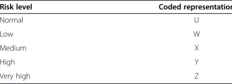
The encoding method processes the sampled output values as individual code. Since working on definite al-phabets is easier than processing numbers with large decimal accuracy, we encode the outputs as a string of alphabets. The alphabetical representation of the five classifications of the outputs is shown in Table 2.

(5)

epoch. A sample output with actual patient readings is shown in Table 3 for eight channels over three epochs.

It can be seen that channel 1 shows low-risk levels while channel 7 shows high-risk levels. Also, the risk level classification varies between adjacent epochs. There are 16 different channels for input to the system at three epochs. This gives a total of 48 input and output pairs. Since we deal with known cases of epileptic patients, it is necessary to find the exact level of epilepsy risk in the patient. This will also aid towards the development of automated systems that can be precisely classify the risk level of the epileptic patient under observation. Hence, an optimization is necessary. This will improve the classification of the patient and can provide the EEG with a clear picture [20]. The outputs from each epoch are not identical and are varying in condition such as [YYZXXXX] to [WYZYYYY] to [YYZZYYY]. In this case, energy factor is predominant and thus results in the high-risk level for two epochs and low-risk level for middle epoch. Channels 5 and 6 settle at high-risk level. Due to this type of mixed state output, we cannot come to a proper conclusion. Therefore, we group four adja-cent channels and optimize the risk level. The frequently repeated patterns show the average-risk level of the group channels. Same individual patterns depict the con-stant risk level associated in a particular epoch. Whether a group of channel is at the high-risk level or not is identified by the occurrences of at least one Z pattern in an epoch. It is also true that the variation of the risk level is abrupt across epochs and eventually in channels. Hence, we are in a dilemma and cannot come up with the final verdict. The five risk levels are encoded as Z >

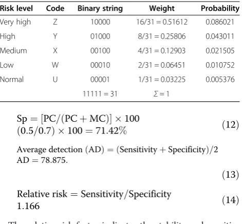
Y > X > W > U in binary strings of length five bits using weighted positional representation as shown in Table 4. Encoding each output risk level gives us a string of seven alphabets, the fitness of which is calculated as the sum of probabilities of the individual alphabets. For example, if the output of an epoch is encoded as ZZYXWZZ, its fitness would be 0.419352.

The performance index of the code converter is given as [19].

PI¼PC‐MC‐FA

PC 100 ð10Þ

Where PI is the performance index, PC is the perfect classification, MC is the missed classification and FA is the false alarm.

The performance of code converter is 44.81%. The perfect classification represents when the physician agrees with the epilepsy risk level. Missed classification represents a high level as low level. False alarm repre-sents a low level as high level with respect to the physi-cian's diagnosis. The other performance measures are also defined as below:

The sensitivity Se and specificity Sp are represented as [19]

Se¼½PC=ðPCþFAÞ 100 0:5=0:6

ð Þ 100¼83:33% ð11Þ

Table 1 Parameter ranges for various risk levels

Normalized parameters

Risk levels

Normal Low Medium High Very high

Energy 0 to 1 0.7 to 3.6 2.9 to 8.2 7.6 to 11 9.2 to 30

Variance 0 to 0.3 0.15 to 0.45 0.4 to 2.2 1.6 to 4.3 3.8 to 10

Peaks 0 to 2 1 to 4 3 to 8 6 to 16 12 to 20

Events 0 to 2 1 to 5 4 to 10 7 to 16 15 to 28

Sharp waves 0 to 2 1 to 5 4 to 8 7 to 11 10 to 12

Average duration 0 to 0.3 0.15 to 0.45 0.4 to 2.4 1.8 to 4.6 3.6 to 10

Covariance 0 to 0.05 0.025 to 0.1 0.09 to 0.4 0.28 to 0.64 0.54 to 1

Table 2 Representation of risk level classifications

Risk level Coded representation

Normal U

Low W

Medium X

High Y

Very high Z

Table 3 Output of code converter for patient 2

Epoch1 Epoch2 Epoch3

WYYWYYY WYYWYYY WZYYWWW

YZZYXXX YYYYXXX YYYXYYY

ZZZYYYY YYYYYYY YYYYYYY

YYZXYYY XZZXYYY YYYYYYY

ZZZYYYY WYYYXXX YYYXYYY

YYZXXXX WYZYYYY YZZYYYY

ZZZYYYY YYYYYYY ZZZYYYY

(6)

Sp¼½PC=ðPCþMCÞ 100 0:5=0:7

ð Þ 100¼71:42% ð12Þ

Average detection ADð Þ ¼ðSensitivityþSpecificityÞ=2 AD¼78:875:

ð13Þ

Relative risk¼Sensitivity=Specificity

1:166 ð14Þ

The relative risk factor indicates the stability and sensitiv-ity of the classifier. For an ideal classifier, the relative risk will be unity. More sensitive classifier will have this factor slightly above unity, whereas slow response classifier makes this factor lower than unity. We have obtained a low value of just 40% for performance index and 83.33%, 71.42%, 78.87%, and 1.166 for sensitivity, specificity, average detec-tion, and relative risk for the code converter. Due to the low performance measures, it is essential to optimize the output of the code converter. Performance index of code converters output using different wavelet transforms for hard thresholding methods are tabulated in Table 5.

2.4 Rhythmicity of code converter

Now, we are about to identify the rhythmicity of code converter techniques which is associated with nonlinearities of the epilepsy risk levels. Let the rhythmicity be defined as [10]

R¼C=D ð15Þ

whereCis the number of categories of patterns andDis the total number of patterns which is 960 in our case. For an ideal classifier, Cis to be one and R= 0.001042. Table 6 shows the rhythmicity of the code converter classifier for hard thresholding of each wavelet. Table 6

shows that the value ofRis highly deviated from its ideal value. Hence, it is necessary to optimize the code converter output to endure a singleton risk level. In the following section, we discuss about the morphological filtering of EEG signals.

2.5 Morphological filtering for feature extraction of EEG signals

Morphological filtering was chosen over other methods such as the temporal approach of the EEG signal and wavelet-based approach due to the fact that morphological filtering can precisely determine the spikes with a very high accuracy rate [14]. Let us call it as a functionf(t). Let us also take into account a structuring element g (t) which together withf(t) be the subsets of Euclidean spaceE.

Accordingly, the Minkowski addition and subtraction [6] for the functionf(t) is given by the relation

Addition:

f⊕g

ð Þð Þ ¼t max t−u∈F u∈G

f tð−uÞ þg uð Þ

f g ð16Þ

Subtraction:

fΘg

ð Þð Þ ¼t min t−u∈F u∈G

f tð−uÞ g uð Þ

f g ð17Þ

The opening and closing functions of the morpho-logical filter is given as:

Opening:

f_g

t

ð Þ ¼fΘgS⊕g ð Þt ð18Þ

Closing:

f•g

ð Þð Þ ¼t f ⊕gSΘg ð Þt ð19Þ

The abovementioned equations help us in determining the peaks and valleys in the original recording [7]. The opening function (erosion-dilation) is used in smoothing of the convex peak of the original signal, and the closing function (dilation-erosion) is used in smoothing the concave peak of the signal. Combinations of opening and closing function lead to the formation of a new filter which when fed with the original signal can divide it into two, the first signal being defined by a structuring element and the second signal being the residue off(t). This type of filtering Table 4 Binary representation of risk levels

Risk level Code Binary string Weight Probability

Very high Z 10000 16/31 = 0.51612 0.086021

High Y 01000 8/31 = 0.25806 0.043011

Medium X 00100 4/31 = 0.12903 0.021505

Low W 00010 2/31 = 0.06451 0.010752

Normal U 00001 1/31 = 0.03225 0.005376

11111 = 31 Σ= 1

Table 5 Performance of code converter output based on wavelet transform along hard thresholding

Wavelets Perfect classification

Missed classification

False alarm

Performance index

Haar 61.45 15.625 22.91 37.58

Db2 61.18 16.14 22.65 36.44

Db4 64.57 12.49 22.91 44.72

Sym8 63.52 11.44 23.95 44.81

Table 6 Rhythmicity of code converter for wavelets with hard thresholding

Wavelets Number of categories of patterns

Rhythmicity

R=C/D

Haar 31 0.032292

Db2 41 0.042708

Db4 30 0.03125

(7)

is done in order to detect the spikes with high accuracy. For two structuring elements, say g1 (t) and g2 (t), the open-close (OC) and close-open (CO) functions are defined as

OCðf tð ÞÞ ¼f tð Þ_g

1ð Þt •g2ð Þt ð20Þ

COðf tð ÞÞ ¼f tð Þ•g₁ð Þt _g

2ð Þt ð21Þ

When considered separately, the OC and CO func-tions result in a variation in amplitude, i.e., while OC results in lower amplitude; the CO function yields higher amplitude. For easier interpretation and calcula-tion, we go for the average of the two defined as opening-closing and closing-opening (OCCO) function. The same is depicted below as

OCCOðf tð ÞÞ ¼½OCðf tð ÞÞ þCOðf tð ÞÞ=2 ð22Þ

f(t) is the original signal represented as

f tð Þ ¼x tð Þ þOCCOðf tð ÞÞ ð23Þ

wherex(t) is the spiky part of the signal.

Performance index, sensitivity, and specificity of code converter outputs through morphological filter-based feature extraction arrived at the low value of 33.46%, 76.23%, and 77.42%, respectively. This scenario impacts the optimization of code converter outputs using postclassifier to accomplish a singleton result. The following section describes about the outcome of SVD, EM, and MEM techniques as postclassifier.

3. Singular value decomposition, expectation maximization, and modified EM as postclassifier for classification of epilepsy risk levels

In this section, we discuss the possible usage of SVD, EM, and MEM as a postclassifier for classification of epilepsy risk levels. The SVD was established in 1870s by Beltrami and Jordan for real square matrices [27]. It is used mainly for dimensionality reduction and deter-mining the modes of a complex linear dynamical system [27]. Since then, SVD is regarded as one of the most important tools of modern numerical analysis and numerical linear algebra.

3.1 SVD theorem

Let us have an m×nmatrix A= [a1, a2, a3…………, an]. The SVD theorem states that [28]:

A¼USVT ð24Þ

whereA∈Rm×n(withm≥n),U∈Rm×n,V∈Rn×n,AndS

is a diagonal matrix of sizeRn×n.

Equation 24 can be further realized as:

A¼XPσkukvTk ð25Þ

The columns ofU are called the left singular vectors of matrixA, and the columns ofVare called the right singular vectors ofA. P= min (m,n) and∑is called as the singular value matrix with along the diagonal.

We have taken the EEG records of 20 patients for our study. Each patient's sample is composed of a 16 × 3 matrix as code converter outputs depicted in Table 3. Considering this to be as matrixA, SVD is computed. The so obtained eigenvalue is eventually regarded as the patient's epilepsy risk level. The similar procedure is carried out in finding out the remaining eigenvalues of other patients as well.

3.2 Expectation maximization as a postclassifier

The EM is often defined as a statistical technique for maxi-mizing complex likelihoods and handling incomplete data problem. EM algorithm consists of two steps namely:

Expectation step (E Step): Say for datax, having an estimate of the parameter and the observed data, the expected value is initially computed [29]. For a given measurement,y1and based on the current estimate

of the parameter, the expected value ofx1is

computed as given below:

x½1kþ1¼E x1jy1;pk

ð26Þ

This implies

x½1kþ1¼y1 1=4

1

4 þp

k

½ 2

ð27Þ

Maximization step (M Step): From the expectation step, we use the data which were actually measured to determine the maximum likelihood (ML) estimate of the parameter.

Considering the code converter output, let us take a set of unit vectors to be asХ. We will have to find out the parametersμandκof the distribution Md (μ,k). Accordingly, we can form the equation as [30]

Х¼fXijXieMdðμ;kÞfor 1≤i≤ng ð28Þ

Consideringxi∈Х, the likelihood ofХis:

PðХjμ;kÞ ¼Pðxi……::xnjμ;kÞ ¼Yn_i_¼1fðxijμ;kÞ ¼Yn_i_¼1cdð Þk ekμ

T_x i

ð29Þ

The log likelihood of Equation25can be written as:

LðХjμ;kÞ ¼ lnPðХjμ;kÞ ¼nlncdð Þ þk kμTr ð30Þ

(8)

In order to obtain the likelihood parametersμandκ, we will have to maximize Equation28with the help of Lagrange operatorλ. The equation can be written as:

Lðμ;λ;κ;ХÞ ¼nlncdð Þ þk kμTrþλð1− μT μÞ

ð31Þ

Derivating Equation29with respect toμ,λ, andκ and equating these to zero will yield the parameter constraints as

^ μ¼ k^

2^λr ð32Þ

^

μT_μ_^_¼₁ _ð₃₃_Þ

nc′ð^kÞ cdð^kÞ

¼−μ^T_r _ð₃₄_Þ

In the expectation step, the threshold data are estimated, given the observed data and current estimate of the model parameters [31]. This is achieved using the conditional expectation,

explaining the choice of terminology. In the M step, the likelihood function is maximized under the assumption that the threshold data are known. The estimate of the missing data from the E step is used in lieu of the actual threshold data.

3.3 Modified expectation maximization algorithm

In this paper, a ML approach uses a modified EM algorithm for pattern optimization. Similar to the conventional EM algorithm, this algorithm alternated between the estimation of the complete loglikelihood function (E step) and the maximization of this estimate over values of the unknown parameters (M step) [32]. Because of the difficulties in the evaluation of the ML function [33], modifications are made to the EM algorithm as follows.

The method of maximum likelihood corresponds to many well-known estimation methods in statistics. For ex-ample, one may be interested in the heights of adult female giraffes, but been unable due to cost or time constraints, to measure the height of every single giraffe in a population. Assuming that the heights are normally (Gaussian) distrib-uted with some unknown mean and variance, the mean and variance can be estimated with MLE while only know-ing the heights of some sample of the overall population.

Given a set of samplesX= {x1,x2…xn}, the complete data set S= (X,Y) consists of the sample set X and a set Yof variable indicating from which component of the mixtures the samples came. The description which is given below ex-plains how to estimate the parameters of the Gaussian mix-tures with the maximization algorithm. After optimization of the patterns, maximum likelihood is adopted to redesign the intracranial area into two clusters. Basically, maximum

likelihood algorithm is a statistical estimation algorithm used for finding log likelihood estimates of parameters in probabilistic models [30].

1. Find the initial values of the maximum likelihood parameters which are mean, covariance, and mixing weights.

2. Assign eachxito its nearest cluster centerck by

Euclidean distance (d).

3. In maximization step, maximization can be used.The likelihood function is written as:

Qθiþ1θi¼ maxQ θiθ ;θiþ1

¼ arg maxQθ;θi ð35Þ d pð ;qÞ ¼d pð ;qÞ ¼

ffiffiffiffiffiffiffiffiffiffiffiffiffiffiffiffiffiffiffiffiffiffiffiffiffiffiffiffiffiffiffi X_n

iþ1ðqi−piÞ

2

q

ð36Þ

4. Repeat iterations and do not stop the loop until it becomes small enough.

The algorithm terminates when the difference between the log likelihood for the previous iteration and current iteration fulfills the tolerance. For μ= 0 and σ= 1, the likelihood function was applied to the 16 × 3 matrix of the code converter output by having truncated to the known endpoints.

4. Results and discussion

To study the relative performance of these code converter and SVD, EM, and MEM, we measure two parameters, the performance index and the quality value. These parameters are calculated for each set of 20 patients and compared.

4.1 Performance index

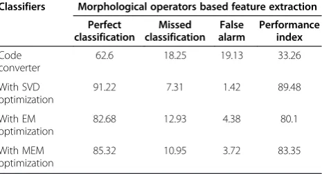
A sample of performance index of morphological filter-based feature extraction with code converters, singular value decomposition, EM, and MEM for an average of 20 known epilepsy data set shown in Table 7. As shown in Table 7, the morphological filter-based feature extraction along with SVD optimization is ranked at first with high PI

Table 7 Performance index for morphological based feature extraction

Classifiers Morphological operators based feature extraction

Perfect classification

Missed classification

False alarm

Performance index

Code converter

62.6 18.25 19.13 33.26

With SVD optimization

91.22 7.31 1.42 89.48

With EM optimization

82.68 12.93 4.38 80.1

With MEM optimization

(9)

of 89.48% against the 80.1% and 83.35% of EM and MEM methods, respectively. But the morphological filter may be plugged into more missed classification rather than less false alarm which is a dangerous trend. Therefore, this method will be considered as a lazy and high threshold classifier.

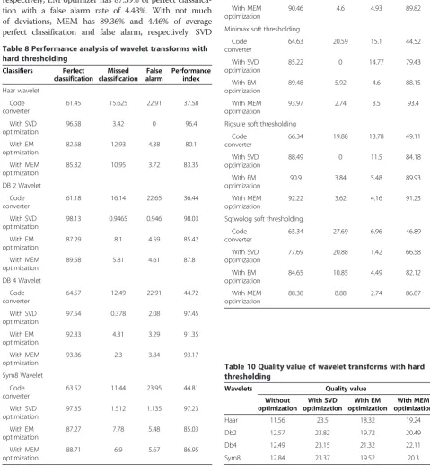
Table 8 depicts the performance analysis of wavelet trans-form with hard thresholding method. In case of hard thresholding, while code converter has got an average classification rate and false alarm of 62.68% and 18.105%, respectively, EM optimizer has 87.39% of perfect classifica-tion with a false alarm rate of 4.43%. With not much of deviations, MEM has 89.36% and 4.46% of average perfect classification and false alarm, respectively. SVD

Table 8 Performance analysis of wavelet transforms with hard thresholding

61.45 15.625 22.91 37.58

96.58 3.42 0 96.4

82.68 12.93 4.38 80.1

85.32 10.95 3.72 83.35

DB 2 Wavelet

Code converter

61.18 16.14 22.65 36.44

98.13 0.9465 0.946 98.03

87.29 8.1 4.59 85.42

89.58 5.81 4.61 87.81

DB 4 Wavelet

Code converter

64.57 12.49 22.91 44.72

97.54 0.378 2.08 97.45

92.33 4.31 3.29 91.35

93.86 2.3 3.84 93.17

Sym8 Wavelet

Code converter

63.52 11.44 23.95 44.81

97.35 1.512 1.135 97.23

87.27 7.78 5.48 85.03

88.71 6.9 5.67 86.95

Table 9 Performance analysis of Haar wavelet transforms with soft thresholding

66.1 19.18 11.93 52.82

87.21 2.84 9.94 82.64

89.03 6.79 4.16 87.88

90.46 4.6 4.93 89.82

Minimax soft thresholding

Code converter

64.63 20.59 15.1 44.52

85.22 0 14.77 79.43

89.48 5.92 4.6 88.15

93.97 2.74 3.5 93.4

Rigsure soft thresholding

Code converter

66.34 19.88 13.78 49.11

88.49 0 11.5 84.18

90.9 3.84 5.48 89.93

92.22 3.62 4.16 91.25

Sqtwolog soft thresholding

Code converter

65.34 27.69 6.96 46.89

77.69 20.88 1.42 66.58

84.65 10.85 4.49 82.12

88.38 8.88 2.74 86.87

Table 10 Quality value of wavelet transforms with hard thresholding

Haar 11.56 23.5 18.32 19.24

Db2 12.57 23.82 19.72 20.49

Db4 12.49 23.15 21.32 22.11

(10)

optimization has the highest value of perfect classification rate of 96.58% with zero false alarms. Hence, SVD optimizer can be regarded as the best postclassifier. In all the four wavelet transforms, SVD postclassifier is the best suited one to achieve the high classification rate. EM and MEM techniques fail miserably to achieve better classifica-tion accuracy when compared with SVD classifier.

Table 9 represents the performance analysis of wavelet transforms with soft thresholding with code converter, SVD, EM, and MEM. It can be found that, in soft thresh-olding, the code converter has an average perfect classifica-tion of 65.6 and false alarm of 11.94. SVD has a classification rate of over 85% with comparatively higher values of false alarms. MEM optimizer claims to be the best optimizer as it has a classification rate of 93.97% with a false alarm rate of 3.5 only. This is obtained when Haar wavelet is used with minimax soft thresholding.

4.2 Quality value

This parameter determines the overall quality of the classi-fiers used. The relation for quality value is given by [19],

QV ¼

C Rfaþ0:2

ð Þ TdlyPdctþ6Pmsd

ð37Þ

WhereCis the scaling constant,Rfais the false alarm per set,Tdly is the average delay of onset classification,Pdct is the percentage of perfect classification, and Pmsd is the percentage of perfect risk level missed.

By setting the value of‘C’to a constant value, say 10, the classifier with the highest QV is the better one. Table 10 depicts the quality value of wavelet transforms with hard thresholding and SVD, EM, and MEM optimization methods. It was observed that SVD with dB2 wavelet in hard thresholding attained the maximum value of QV at 23.82, and EM with Haar wavelet has the low value of QV at 18.32.

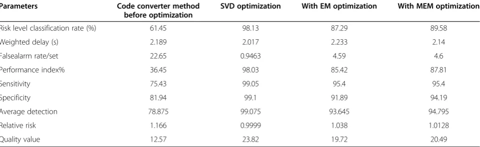
Table 11 shows the performance analysis of 20 patients using dB2 wavelet hard thresholding with SVD, EM, and MEM as postclassifiers. The evaluation parameters achieved an appreciable value in the case of SVD postclassi-fier when compared to the other two classipostclassi-fiers. Hence, we can choose SVD as a good postclassifier for epilepsy risk level classification. All the three postclassifiers are bestowed with the best sensitivity and specificity measures. EM and MEM classifiers are plugged into the higher false alarm rate, and this leads to the lower QV and PI for the system.

Since the Haar wavelet is a predominant wavelet, we had chosen this wavelet for the four types of soft thresholding methods and the same is depicted in Table 12. As seen in Table 12, the highest QV of 22.54 is attained in the minimax soft thresholding with MEM as a postclassifier.

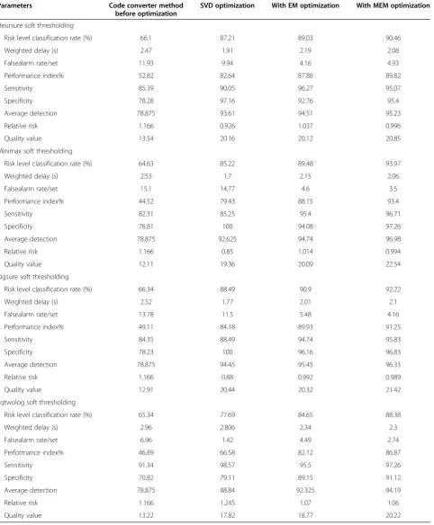
Table 13 exhibits the performance analysis of 20 patients using Haar wavelet in soft thresholding with SVD, EM, and MEM postclassifiers. MEM postclassifier with minimax soft thresholding reached the better QV and PI when compared to SVD and EM classifiers. A slight incremental tradeoff in the weighted delay for MEM is responsible for this perfor-mancewhen comparedwith SVD and EM classifiers. SVD fails to achieve a good performance in this methodology due to more false alarm rate. EM is struck in the middle path as far as performance index is concerned.

Table 14 shows the performance analysis of 20 patients using morphological filters with SVD, EM, and MEM Table 11 Performance analysis of twenty patients using db2 wavelet hard thresholding with SVD, EM, and MEM postclassifiers

Parameters Code converter method before optimization

SVD optimization With EM optimization With MEM optimization

Risk level classification rate (%) 61.45 98.13 87.29 89.58

Weighted delay (s) 2.189 2.017 2.233 2.14

Falsealarm rate/set 22.65 0.9463 4.59 4.6

Performance index% 36.45 98.03 85.42 87.81

Sensitivity 75.43 99.05 95.4 95.4

Specificity 81.94 99.1 91.89 94.19

Average detection 78.875 99.075 93.645 94.795

Relative risk 1.166 0.9999 1.038 1.0128

Quality value 12.57 23.82 19.72 20.49

Table 12 Quality value of Haar wavelet transforms with soft thresholding

Haar wavelet with soft thresholding

Quality value

Code converter

Heursure 13.54 20.16 20.12 20.85

Mini max 12.11 19.38 20.09 22.54

Rigsure 12.91 20.44 20.32 21.42

(11)

Table 13 Performance analysis of 20 patients using Haar wavelet in soft thresholding with SVD, EM, and MEM postclassifiers

Parameters Code converter method before optimization

SVD optimization With EM optimization With MEM optimization

Heursure soft thresholding

Weighted delay (s) 2.47 1.91 2.19 2.08

Sensitivity 85.39 90.05 96.27 95.07

Specificity 78.28 97.16 92.76 95.4

Relative risk 1.166 0.926 1.037 0.996

Quality value 13.54 20.16 20.12 20.85

Minimax soft thresholding

Weighted delay (s) 2.53 1.7 2.15 2.06

Sensitivity 82.31 85.25 95.4 96.71

Specificity 76.81 100 94.08 97.26

Relative risk 1.166 0.85 1.014 0.994

Quality value 12.11 19.36 20.09 22.54

Rigsure soft thresholding

Weighted delay (s) 2.52 1.77 2.01 2.1

Sensitivity 84.35 88.49 94.74 95.83

Specificity 78.23 100 96.16 96.83

Relative risk 1.166 0.88 0.992 0.989

Quality value 12.91 20.44 20.32 21.42

Sqtwolog soft thresholding

Weighted delay (s) 2.96 2.806 2.34 2.3

Sensitivity 91.34 98.57 95.5 97.26

Specificity 70.82 79.11 89.15 91.12

Relative risk 1.166 1.245 1.07 1.06

(12)

postclassifiers. In this method, SVD outperforms other clas-sifiers in terms of QV and PI. This morphological filtering is inherited with slow response and is considered to be a high-threshold classifier. SVD classifier is summed with low false alarm and weighted delays. All these methods are in an average, positioned at more than 90% of performance index, and around quality value of 18. Since for all these classifiers, the obtained weighted delay is more than 2 s; it leads to larger threshold and slow response system.

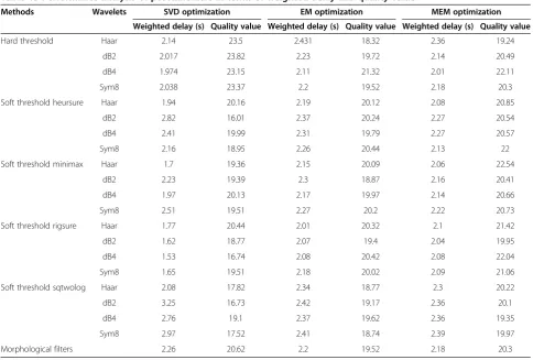
We wish to analyze the time complexity of the postclassi-fiers in terms of weighted delay and quality value. Table 15

shows the performance analysis of postclassifiers in terms of weighted delay and quality value. It is observed that the four types of wavelet transforms in hard thresholding method along with SVD postclassifier attained low weighted delay and high value of QV.

In the case of Table 15, the EM and MEM classifiers are either plugged into more missed classification or false alarms and subsequently leads to lower value of QV less than 20 in most of the wavelet transforms. In case of soft thresholding, dB2 wavelet in rigsure thresholding for MEM postclassifier outperforms other fifteen methods. Table 14 Performance analysis of 20 patients using morphological filters with SVD, EM, and MEM postclassifiers

Parameters Code converter method SVD optimization With EM optimization With MEM optimization

Weighted delay (s) 2.34 2.26 2.2 2.18

Sensitivity 77.84 98.57 95.59 98.97

Specificity 78.91 92.65 98.11 97.67

Relative risk 1.166 1.063 0.974 1.013

Quality value 12.74 20.62 19.52 20.3

Table 15 Performance analysis of postclassifiers in terms of weighted delay and quality value

Methods Wavelets SVD optimization EM optimization MEM optimization

Weighted delay (s) Quality value Weighted delay (s) Quality value Weighted delay (s) Quality value

Hard threshold Haar 2.14 23.5 2.431 18.32 2.36 19.24

dB2 2.017 23.82 2.23 19.72 2.14 20.49

dB4 1.974 23.15 2.11 21.32 2.01 22.11

Sym8 2.038 23.37 2.2 19.52 2.18 20.3

Soft threshold heursure Haar 1.94 20.16 2.19 20.12 2.08 20.85

dB2 2.82 16.01 2.37 20.24 2.27 20.54

dB4 2.41 19.99 2.31 19.79 2.27 20.57

Sym8 2.16 18.95 2.26 20.44 2.13 22

Soft threshold minimax Haar 1.7 19.36 2.15 20.09 2.06 22.54

dB2 2.23 19.39 2.3 18.87 2.16 20.41

dB4 1.97 20.13 2.17 19.97 2.14 20.66

Sym8 2.51 19.51 2.27 20.2 2.22 20.73

Soft threshold rigsure Haar 1.77 20.44 2.01 20.32 2.1 21.42

dB2 1.62 18.77 2.07 19.4 2.04 19.95

dB4 1.53 16.74 2.08 20.42 2.08 22.04

Sym8 1.65 19.51 2.18 20.02 2.09 21.06

Soft threshold sqtwolog Haar 2.08 17.82 2.34 18.77 2.3 20.22

dB2 3.25 16.73 2.42 19.17 2.36 20.1

dB4 2.76 19.1 2.37 19.62 2.36 19.35

Sym8 2.97 17.52 2.41 18.74 2.39 19.97

(13)

Morphological filters are stacked at higher delay with QV set at near 20.

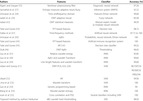
Table 16 shows a good collection of recent papers in this area are given in the review paper by Rajendra Acharya etal. in [34]. Studies that presented techniques for two-class (normal, ictal) epilepsy activity classification are that of Nigam and Graupe [35] who used a multistage nonlinear pre-processing filter along with an artificial neural network (ANN) for the automated detection of epileptic signals and obtained an accuracy of around 97.20%. Nonlinear parame-ters like CD, LLE, H, and entropy were used to characterize the EEG signal and discriminate epileptic and alcoholic EEG from normal EEG with more than 90%accuracy [36]. Using the same dataset, the same group automatically clas-sified EEG signals into normal and epileptic using different entropies using an adaptive neuro-fuzzy interference sys-tem(ANFIS) and obtained an accuracy of 92.22% [37]. Time domain and frequency domain EEG features combined with Elman network were used to classify the two classes with an accuracy, sensitivity, and specificity of 99.6% [38]. Normal and epileptic EEG signals were automatically iden-tified with a classification accuracy of85.9% using discrete wavelet transform (DWT) sub-band energy as input

features to adaptive neural fuzzy network [39]. Srinivasan et al. [40] developed an automated epileptic EEG detection system using approximate entropy as the feature in Elman and probabilistic neural networks. Elman network yielded an overall accuracy of 100%. Tzallas et al. [41] employed time-frequency methods to analyze selected segments of EEG signals for automated detection of seizure using neural network and obtained an accuracy ranging from 97.72% to 100%. Subasi [42] applied DWT on EEG signals and decomposed them into frequency sub-bands. DWT coeffi-cients were converted into four statistical features, and these were fed to a modular neural network called mixture of experts (MEs). They classified normal and epileptic EEG signals with an accuracy of 94.5%, sensitivity of 95%, and specificity of 94%. Polat and Gunes [43] classified EEG sig-nals into epileptic and normal using fast Fourier transform (FFT)-based Welch method and decision tree classifier and achieved a maximum classification accuracy of 98.72%, sensitivity of 99.4%, and specificity of 99.31%. The same group [44] used the Welch FFT method for feature extrac-tion, PCA for dimensionality reducextrac-tion, and a new hybrid automated identification system based on artificial immune recognition system (AIRS) with fuzzy resource allocation

Table 16 Summary of previous works for automated detection of normal and epileptic classes

Authors Features Classifier Accuracy (%)

Nigam and Graupe [35] Nonlinear preprocessing filter Diagnostic neural network 97.20

Kannathal et al. [37] Entropy measures adaptive neuro-fuzzy Inference system (ANFIS) 92.22

Srinivasan et al. [38] Time andfrequency domain Features Elman network 99.60

Sadati et al. [39] DWT adaptive neural Fuzzy network 85.90

Subasi [42] DWT statistical measures Mixture expert model

(a modular neural network)

94.50

Polat and Gunes [43] FFT-based features Decision tree 98.72

Tzallas et al. [41] Time-frequency methods Artificial neural network 97.72 to 100

Srinivasan et al. [40] ApEn Probabilistic neural network, Elman network 100

Polat and Gunes [44] FFT-based features Artificial immune recognition system 100

Polat and Gunes [45] AR C4.5 Decision tree classifier 99.32

Ocak [46] DWT-ApEn Thresholding 96.65

Guo et al. [47] Relative wavelet energy ANN 95.85

Guo et al. [48] ApEn and wavelet Transform ANN 99.85

Guo et al. [49] Line length features and wavelet transform ANN 99.60

Subasi and Gursoy [51] DWT-PCA, ICA, LDA SVM 98.75(PCA)

99.50(ICA)

100(LDA)

Ubeyli [52] AR SVM 99.56

Lima et al. [53] Wavelet transform SVM 100

Guo et al. [50] Genetic programming based KNN 99

Wang et al. [54] Wavelet packet entropy KNN 100

Iscan et al. [55] Cross correlation and PSD Several classifiers including SVM 100

(14)

mechanism for classification of normal and epileptic seg-ments. They reported an accuracy of 100%.The same group ([45] used autoregressive (AR) for feature extraction and C4.5 decision tree classifier for classification and reported an accuracy of99.32%. Ocak [46] developed a method for automated seizure detection based on ApEn and DWT. They were able to distinguish seizures with more than 96% accuracy. Guo et al.conducted many studies using ANN for classification and reported an accuracy of95.2%, sensitivity of 98.17%, and specificity of 92.12% using relative wavelet energy-based features [47]; an accuracy of 99.85%, sensitiv-ity of 100%, and specificsensitiv-ity of 99.2% using wavelet trans-form and ApEn features [48]; an accuracy of 99.60% using wavelet transform and line length feature [49]; and an accuracy of 99% using genetic programming-based features in a K-nearest neighbor (KNN)classifier [50]. The DWT features were reduced using PCA, ICA, andLDA, and the resultant features were used to classify normal andepilepsy EEG signals using SVM classifier [51]. They obtained an ac-curacy of 98.85% using PCA method,99.5% using ICA method, and 100% using LDA method. Ubeyli [52] used AR methods for feature extraction and SVM for classifica-tionand reported an accuracy of 99.56%. In other recent studies, 100% classification accuracy was achieved by Lima et al. [53] (wavelet transform and SVM), Wang et al. [54] (wavelet packet entropy and KNN), Iscan et al. [55] (cross correlation and PSDand SVM), and Orhan et al. [56] (DWT and ANN). Finally, the proposed system by authors used seven parameters along with wavelet hard threshold-ing and obtained an accuracy of 99.03%, sensitivityof 99.05%,and specificity of 99.1%.Table 16 gives a summary of the above listed studies for automated detection of nor-mal and epileptic classes. It can be observed that a variety of methods like FFT, time-frequency, DWT, morphological filtering,wavelet, statisticalmeasures, nonlinear, chaotic, and entropy measures, and dimension reduction methods like PCA, ICA,SVD,EM,MEM, and LDA are used to analy-zeEEG to detect epileptic state from normal state.

5 Conclusions

The objective of this paper is to classify the risk level of the epileptic patients from the EEG signals. The aim is to obtain high classification rate, performance index, quality value with low false alarm, and missed classification. Due to the nonlinearity obtained and also the poor performance found in the code converters, an optimization was vital for the effective classification of the signals. We opted SVD, EM, and MEM as postclassifiers. Morphological filters were also used for the feature extraction of the EEG signals. After having computed the values of PI and QV discussed under the results column, we found that SVD was working per-fectly with a high classification rate of 91.22% and a false alarm as low as 1.42. Therefore, SVD was chosen to be the best postclassifier. The accuracy of the results obtained can

be made even better by using extreme learning machine as a postclassifier, and further research will be in this direction.

Competing interests

The authors declare that they have no competing interests.

Acknowledgements

The authors express their sincere thanks to the Management and the Principal of Bannari Amman Institute of Technology, Sathyamangalam for providing the necessary facilities for the completion of this paper. This research is also funded by AICTE RPS: F. No 8023/BOR/RID/RPS-41/2009-10, dated 10 Dec 2010.

Received: 24 August 2013 Accepted: 10 April 2014 Published: 3 May 2014

References

1. Y Yuan,Detection of Epileptic Seizure Based on EEG Signals, 3rd International Congress on Image and Signal Processing (CISP2010), and IEEE(IEEE, Piscataway, 2010), pp. 4209–4211

2. S Herculano-Houzel, The human brain in numbers: a linearly scaled-up primate brain. Front. Hum. Neurosci.3, 1–11 (2009). doi:3389/neuro.09.031.2009 3. Z Zainuddin, L KeeHuong, P Ong, On the use of wavelet neural networks in

the task of epileptic seizure detection from electroencephalography signals, proceedings of the 3rd International Conference on Computational Systems. Biol. Bioinformatics.11, 149–159 (2012)

4. AA Dingle, RD Jones, GJ Carroll, RR Fright, A multistage system to detect epileptic form activity in the EEG. IEEE Trans. Biomed. Eng.40(12), 1260–1268 (1993)

5. R Harikumar, R Sukanesh, PA Bharathi, Genetic algorithm optimization of fuzzy outputs for classification of epilepsy risk levels from EEG signals. J. Interdiscip. Panels I.E.(India)86(1), 1–10 (2005)

6. P Xanthopoulos, S Rebennack, CC Liu, J Zhang, GL Holmes, BM Uthman, PM Pardalos, A novel wavelet based algorithm for spike and wave detection in absence of epilepsy, inProc of IEEE International Conference on Bio informatics and Bio Engg(IEEE, Piscataway, 2006), pp. 14–19

7. A Mirzaei, A Ayatollahi, P Gifani, L Salehi, EEG analysis based on wavelet-spectral entropy for epileptic seizures detection, inProc. of 3rd International Conference on Biomedical Engineering and Informatics(BMEI 2010); Changai, January 2010(IEEE, Piscataway, 2010), pp. 878–882

8. PE McSharry, LA Smith, L Tarassenko, Prediction of epileptic seizures: are non linear methods relevant? Nat. Med.9, 241–242 (2003)

9. J Gotman, Automatic seizure detection: improvements and evaluation. Electroencephalogr. Clin. Neurophysiol.76, 317–324 (1990)

10. CCC Pang, ARM Upton, G Shine, MV Kamath, A comparison of algorithms for detection of spikes in the electroencephalogram. IEEE Trans. BME50(4), 521–526 (2003)

11. L Tarassenko, YU Khan, MRG Holt, Identification of inter-ictal spikes in the EEG using neural network analysis. IEE Proc. Sci. Meas. Technol.

145, 270–278 (1998)

12. M van Gils, Signal processing in prolonged EEG recordings during intensive care. IEEE EMB Mag.16(6), 56–63 (1997)

13. E Sezer, H Isik, E Saracoglu, Employment and comparison of different artificial neural networks for epilepsy diagnosis from EEG signals. J. Med. Syst.36(1), 347–362 (2012)

14. A Rezasarang, A strong adaptive and comprehensive evaluation of wavelet based epileptic EEG spike detection methods, inProc.of International conference on Bio medical and Pharmaceutical Engineering, (ICBPE 2006) Singapore, 2006(IEEE, Piscataway, 2006), pp. 432–437

15. K Majumdar, Human scalp EEG processing: various soft computing approaches. Appl. Soft Comput.11(8), 4433–4447 (2011)

16. RP Costa, P Oliveria, G Rodrigues, L Burno, A Burno, Epileptic seizure classification using neural networks with 14 features, inProceedings of the 12th International Conference on Knowledge Based Intelligent Information and Engineering System, Zageed, Croatia, Part II Lecture Notes of Computer Science Series(Springer, Heidelberg, Germany, 2008), pp. 281–288

(15)

18. WRS Webber, RP Lesser, RT Richardson, K Wilson, An approach to seizure detection using an artificial neural network (ANN). Electroencephalogr. Clin. Neurophysiol.98, 250–272 (1996)

19. H Qu, J Gotman, A patient specific algorithm for detection onset in long-term EEG monitoring-possible use as warning device. IEEE Trans. Biomed. Eng.44(2), 115–122 (1997)

20. R Harikumar, T Vijayakumar, MG Sreejith, Performance analysis of SVD and support vector machines for optimization of fuzzy outputs in classification of epilepsy risk level from EEG signals, inIEEE Conference on Recent Advances in Intelligent Computational Systems (RAICS) RAICS.201; Trivandrum, India

(IEEE, Piscataway, 2009), pp. 718–728

21. RM Rangayyan,Biomedical Signal Analysis a Case Study Approach(IEEE Press-John Wiley, New York, 2002)

22. LM Patnaik, OK Manyam, Epileptic EEG detection using neural networks and post classification. Comput. Methods Programs Biomed.91, 100–109 (2008) 23. AT Tzallas, MG Tsipouras, DI Fotiadis, A time-frequency based method for

the detection of epileptic seizure in EEG recording, in12th IEEE International Symposium on Computer based Medical Systems (CBMS’07); Melbourn, Australia(IEEE, Piscataway, 2007), pp. 23_–27

24. VVKDV Prasad, P Siddiah, B Prabhakararao, A new wavelet based method for denoising biological signals. Int. J. Comput. Sci. Netw. Secur.8(1), 238_–244 (2008)

25. P Kumar, D Agnihotri, Bio signal denoising via wavelet thresholds. IETE J. Res.56(3), 132–138 (2010)

26. R Harikumar, B Sabarish Narayanan, Fuzzy techniques for classification of epilepsy risk level from EEG signals, inProceedings of IEEE Tencon_–2003, Bangalore, India, 14–17 October 2003(IEEE, Piscataway, 2003), pp. 209–213 27. VC Klema, AJ Laub, The singular value decomposition: its computation and

some applications. IEEE Trans. Autom. Control Ac25(2), 164–176 (1980) 28. PK Sadasivam, D Narayana Dutt, SVD based technique for noise reduction in

electroencephalographic signal. Signal Process.55, 179–189 (1996) 29. TK Moon, The expectation maximization algorithm in signal processing.

IEEE Signal Process. Mag.13(6), 47–60 (1996)

30. CE Mc, Culloch, Maximum likelihood algorithm for generalized linear mixed models. J. Am. Stat. Assoc.92, 162–170 (1991)

31. GJ Tian, Y Xia, Y Zhang, D Feng, Hybrid genetic and variational expectation-maximization algorithm for Gaussian-mixture-model-based brain MR image segmentation. IEEE Trans. Inf. Technol. Biomed.15(3), 373–380 (2011)

32. Y Zhou, P Jim, Y Lee, A modified expectation maximization algorithm for maximum likelihood. IEEE Conf. Signals Syst. Comput.1, 613_–617 (2000) 33. X Jinlong, L Jianwu, Y Yang, A new EM acceleration algorithm for multi-user

detection. IEEE Int. Conf. Measuring Technol. Mechatronics Automation1, 150_–153 (2011)

34. U Rajendra Acharya, S Vinitha Sree, G Swapna, RJ Martis, JS Suri, Automated EEG analysis of epilepsy: a review. Knowl. Based Syst.45, 147–165 (2013) 35. VP Nigam, D Graupe, A neural-network-based detection of epilepsy. Neurol.

Res.26(1), 55_–60 (2004)

36. N Kannathal, UR Acharya, CM Lim, Q Weiming, M Hidayat, PK Sadasivan, Characterization of EEG: a comparative study. Comput. Methods Programs Biomed.80(1), 17_–23 (2005)

37. N Kannathal, CM Lim, UR Acharya, PK Sadasivan, Entropies for detection of epilepsy in EEG. Comput. Methods Programs Biomed.80(3), 187–194 (2005) 38. V Srinivasan, C Eswaran, N Sriraam, Artificial neural network based epileptic

detection using time-domain and frequency domain features. J. Med. Syst.

29(6), 647–660 (2005)

39. N Sadati, HR Mohseni, A Magshoudi, Epileptic seizure detection using neural fuzzy networks, inProceedings of the IEEE International Conference on Fuzzy Systems; Taiwan, 2006(IEEE, Pisctawaya, 2006), pp. 596–600

40. V Srinivasan, C Eswaran, N Sriraam, Approximate entropy-based epileptic EEG detection using artificial neural networks. IEEE Trans. Inform. Technol. Biomed.11(3), 288–295 (2007)

41. AT Tzallas, MG Tsipouras, DI Fotiadis, Automatic seizure detection based on time-frequency analysis and artificial neural networks. Comput. Intell. Neurosci. (2007). http://dx.doi.org/10.1155/2007/80510

42. A Subasi, EEG Signal classification using wavelet feature extraction and a mixture of expert model. Expert Syst. Appl.32(4), 1084–1093 (2007) 43. K Polat, S Gunes, Classification of epileptiform EEG using a hybrid systems

based on decision tree classifier and fast Fourier transform. Appl. Math. Comput.187(2), 1017–1026 (2007)

44. K Polat, S Gunes, Artificial immune recognition system with fuzzy resource allocation mechanism classifier, principal component analysis and FFT method based new hybrid automated identification system for classification of EEG signals. Expert Syst. Appl.34(3), 2039–2048 (2008)

45. K Polat, S Gunes, A novel data reduction method: distance based data reduction and its application to classification of epileptiform EEG signals. Appl. Math. Comput.200(1), 10–27 (2008)

46. H Ocak, Automatic detection of epileptic seizures in EEG using discrete wavelet transform and approximate entropy. Expert Syst. Appl.

36(2), 2027–2036 (2009)

47. L Guo, D Rivero, JA Seoane, A Pazos, Classification of EEG signals using relative wavelet energy and artificial neural networks, inConf Proc of the First ACM/SIGEVO Summit on Genetic and, Evolutionary Computation; Changai, 2009(IEEE, Piscataway, 2009), pp. 177–184

48. L Guo, D Rivero, A Pazos, Epileptic seizure detection using multiwavelet transform based approximate entropy and artificial neural networks. J. Neurosci. Methods193(1), 156–163 (2010)

49. L Guo, D Rivero, J Dorado, JR Rabunal, A Pazos, Automatic epileptic seizure detection in EEGs based on line length feature and artificial neural networks. J. Neurosci. Methods191(1), 101–109 (2010)

50. L Guo, D Rivero, J Dorado, CR Munteanu, A Pazos, Automatic feature extraction using genetic programming: an application to epileptic EEG classification. Expert Syst. Appl.38(8), 10425–10436 (2011)

51. A Subasi, MI Gursoy, EEG signal classification using PCA, ICA, LDA and support vector machine. Expert Syst. Appl.37(12), 8659–8686 (2010) 52. ED Ubeyli, Least squares support vector machine employing model-based

methods coefficients for analysis of EEG signals. Expert Syst. Appl.37(1), 233–239 (2010)

53. CA Lima, AL Coelho, M Eisencraft, Tackling EEG signal classification with least squares support vector machines: a sensitivity analysis study. Comput. Biol. Med.40(8), 705–714 (2010)

54. D Wang, D Miao, C Xie, Best basis-based wavelet packet entropy feature extraction and hierarchical EEG classification for epileptic detection. Expert Syst. Appl.38(11), 14314–14320 (2011)

55. Z Iscan, Z Dokur, D Tamer, Classification of electroencephalogram signals with combined time and frequency features. Expert Syst. Appl.38(8), 10499–10505 (2011)

56. U Orhan, M Hekim, M Ozer, EEG signals classification using the K-means clustering and a multilayer perceptron neural network model. Expert Syst. Appl.38(10), 13475–13481 (2011)

doi:10.1186/1687-6180-2014-59

Cite this article as:Harikumar and Vijayakumar:Performance analysis of wavelet transforms and morphological operator-based classification of

epilepsy risk levels.EURASIP Journal on Advances in Signal Processing

20142014:59.