Application of ground scatter returns for calibration of HF interferometry data

F U L L P A P E R

Open Access

Application of ground scatter returns for

calibration of HF interferometry data

Pavlo Ponomarenko

, Nozomu Nishitani

, Alexey V. Oinats

, Taishi Tsuya

and Jean-Pierre St.-Maurice

Abstract

Information on the vertical angle of arrival (elevation) is crucial in determining propagation modes of high-frequency (HF, 3–30 MHz) radio waves travelling through the ionosphere. The most advanced network of ionospheric HF radars, SuperDARN (Super Dual Auroral Radar Network), relies on interferometry to measure elevation, but this information is rarely used due to intrinsic difficulties with phase calibration as well as with the physical interpretation of the measured elevation patterns. In this work, we propose an empirical method of calibration for SuperDARN interferometry. The method utilises a well-defined dependence of elevation on range of ground scatter returns.“Fine tuning”of the phase is achieved based on a detailed analysis of phase fluctuation effects at very low elevation angles. The proposed technique has been successfully applied to data from the mid-latitude Hokkaido East SuperDARN radar. It can also be used at any other installation that utilises HF interferometry.

Keywords:Ionospheric radio wave propagation; High-frequency radars; Interferometry

Background

High-frequency (HF, 10–20 MHz) radars are actively used for monitoring ionospheric conditions at high and mid-latitudes and provide information on plasma dy-namics (drifts, diffusion etc.) at E- and F-region heights. Currently, the most advanced instrument in this cat-egory is the Super Dual Auroral Radar Network (Super-DARN) which covers high to mid-latitude regions in both hemispheres (Greenwald et al. 1995, Chisham et al. 2007). SuperDARN typically consists of pairs of radars with overlapping fields of view which allows for the esti-mate of a horizontal vector of ionospheric plasma drift based on the Doppler frequency shift of the ionospheric backscatter returns. This information is used for the re-construction of ionospheric electric potential at F-region heights (Ruohoniemi and Baker 1998).

One of the most important tasks in the interpretation of the HF echoes is to establish their propagation mode so that the Doppler shift information can be correctly converted into electric field. Among the multitude of the HF propagation modes existing in the ionosphere, the conventional software distinguishes only between the

ionospheric and ground scatter (Blanchard et al. 2009). Much more detailed and accurate propagation informa-tion can be obtained from the dependence of elevainforma-tion angle as a function of range (e.g. Kelso 1964). These data are actually available for most of the SuperDARN radars, for which elevation is estimated from the phase delay be-tween two spatially separated antenna arrays (Greenwald et al. 1995, Milan et al. 1997). And yet, while the elevation data have been recorded since the inception of Super-DARN, they have rarely been used until recently due to inherent technical difficulties related to the phase calibra-tion of the HF arrays, e.g. using a standard source located at a fixed elevation. Furthermore, while the phase offset between the interferometer arrays has to be carefully re-evaluated after each hardware and software update, it is also a subject to gradual changes in the physical proper-ties of the antennas, cables, and electric circuitry. There-fore, there is a pressing need in a simple but reliable way of monitoring these changes.

In this work, we lay the physical and statistical foun-dations for empirically estimating the phase offsets in SuperDARN data. The proposed approach was thor-oughly tested and then applied to Hokkaido East data allowing for the physically justified estimation of the elevation, which considerably extends diagnostic capabil-ities of the network.

* Correspondence:[email protected]

1

Solar-Terrestrial Environment Laboratory, Nagoya University, Nagoya, Japan

3_{University of Saskatchewan, Saskatoon, SK, Canada}

Full list of author information is available at the end of the article

Methods

SuperDARN interferometry

The main array of SuperDARN radars is used both for radio wave emission and reception of echoes. It contains a line of 16 elements (either log-periodic director anten-nas or broad-band wire dipoles), which are separated by ≈15 m. The horizontal alignment of the array elements produces a knife-like diagram which is relatively narrow in the azimuthal plane and broad in the vertical plane. Scanning (beam-forming) in azimuth is achieved by applying a linear phase shift between array elements. Usually, SuperDARN arrays scan consecutively through 16 azimuthal directions (beams) within ±27° from the boresight direction. Elevation selection is based on measuring phase shiftΨbetween the echoes received by the main array and an auxiliary (interferometer) array. The latter consists of four elements and is usually lo-cated at 100 m in front of or behind the main array (Fig. 1). Both arrays form beams pointing in the same azimuthal direction so that the narrower beam from the main array is “embedded” into the wider interfer-ometer beam. The elevation angle is calculated as Δ= cos−1[Ψ/kdcosϕ], where k= 2π/λ is the radar wave vector magnitude, d is the interferometer base and φ is azimuth measured from the boresight direction (Milan et al. 1997).

There is an intrinsic ambiguity arising from the fact that the interferometer base of d= 100 m is larger than the radar wavelength,λ≈20–30 m. As a result, the max-imum phase shift (observed at zero elevation),Ψmax=kd

cosϕ, lies between 6π and 10π, while instrumentally the phase can only be measured between −π and +π. Figure 2 shows the relationship between elevation and phase shift for central beams (φ= 0) at the typical Hokkaido East frequency of 11 MHz. The black line shows the total phase shift while the blue lines corres-pond to the actually measured phase shift which is confined to within ±π range. The latter illustrates the above-mentioned ambiguity with the same phase shift corresponding to multiple elevation values.

The ionospheric scatter echoes are expected to come from anisotropic plasma irregularities aligned with the geomagnetic field lines, and the maximum backscatter power is observed when the radio wave propagates in the direction orthogonal to the field lines. At high latitudes, the field lines are nearly vertical so that the backscatter elevation is expected to be closer to the hori-zontal direction, somewhere between 0 and 30°–40°. As a result, in SuperDARN software, the assumption made that the echoes come from within the first segment, i.e. betweenΨmax−2πandΨmax,and the resulting elevation

estimates lie between zero and some maximum value Δ2π= cos−1[(Ψmax−2π)/Ψmax] (Milan et al. 1997). This

phase shift range is highlighted by red in Fig. 2.

Theoretical dependence of elevation vs range for ground scatter

In order to estimate a phase offset, first we need to iden-tify an expected pattern for a known propagation mode of the radio wave. In order to produce plasma circula-tion maps, SuperDARN utilises HF backscatter returns from small-scale ionospheric irregularities (ionospheric scatter, IS). Importantly, spatio-temporal characteristics of IS are subject to different kinds of plasma instabilities which may or may not be present in the radar’s field-of-view, in contrast to the regular ground scatter (GS) echoes, which represent radio waves “reflected” by the regular ionospheric layer before they are scattered back by the rugged ground surface. While GS echoes are treated as interference by SuperDARN data processing procedures, their regular character makes this propaga-tion mode very useful as a reference in analysing inter-ferometer phase patterns.

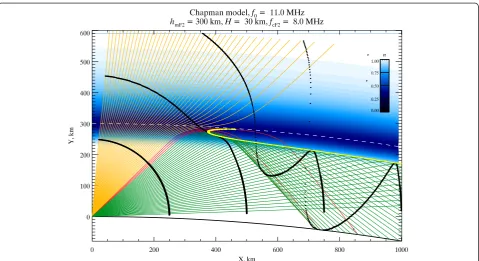
Figure 3 represents a ray tracing simulation of HF propagation in a simplified situation of a single Chapman layer with a maximum density located at 300-km altitude and a scale height of 30 km. The ray tracing code was de-veloped by Ponomarenko et al. (2009) and utilises Snell’s law and the simplest form of the Appleton-Hartree

Fig. 1Hokkaido East SuperDARN radar antennas

Fig. 2Transfer function between interferometer phase shift and elevation angle obtained for the boresight direction of the radar antenna. Theblack curveshows total phase shift for the given interferometer base of 100 m and a typical Hokkaido radar frequency of 11 MHz for the elevation range between 0° and 90° (for the remaining back-lobe range 90°–180°, the dependence should be mirrored around 90° elevation and zero phase). Theblue linecorresponds to the measured phase confined to the ±πinterval and shows that a single measured phase value corresponds to multiple elevation angles. The conventional 2πrange used for calculating SuperDARN elevation is highlighted byred

equation, n2_¼1−f2

p=f

2

0, where f0 and fp are the wave

frequency and plasma frequency, respectively. The ray trajectories were simulated between 0° and 85° separated by 0.1° in elevation at the radar location. The physical range resolution is 1 km (in Fig. 3, the rays are plotted at 1° intervals only). The blue shading shows the spatial dis-tribution of the ionospheric refractive index. The black dots show group range in 250-km steps. There are three major propagation modes: (i) low-angle rays (green), (ii) high-angle (Pedersen) rays (red), and (iii) escaping rays (orange). While all three propagation modes can contrib-ute to IS, only the first two reach the ground and are capable of generating GS. The yellow contour corresponds to the turning (“reflection”) points of the rays with the top and bottom branches produced by the Pedersen and low-angle rays, respectively, while their convergence point at close ranges corresponds to the skip zone boundary on the ground. The Pedersen mode covers a narrow angular range (≈3° in this case) and corresponds to divergent rays “gliding” along the ionospheric maximum. This contrasts with the low-angle mechanism covering a comparatively large angular range and producing significantly larger power density due to convergent rays“reflected”from the bottom part of the ionospheric layer.

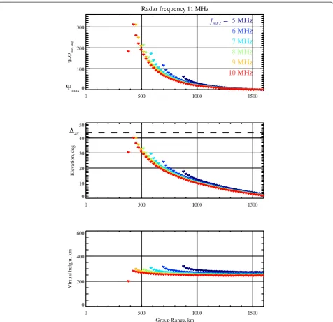
As a consequence of the larger ray/power density, the low-ray mode is expected to dominate GS returns. This assumption is supported by analysing simulated GS eleva-tion at each 45-km range gate. The median value for all trajectories reaching the ground was estimated within each 45-km range of group delays. The result is presented in the middle panel of Fig. 4. Here, different colours correspond to different maximum plasma frequencies in-creasing from 5 to 10 MHz (dark blue to red) in 1-MHz steps. The elevation values gradually decrease with increasing range until they approach zero level, as would be expected from the low-angle mode. The horizontal dash line shows the maximum measured elevation, Δ2_π. The top panel in Fig. 4 shows respective phase shift values. For convenience, the phase was shifted by the maximum possible phase value, namely (Ψ-Ψmax), so that a smaller

phase shift corresponds to a lower elevation and vice versa. The bottom panel shows the respective values of the virtual height calculated from the group range r

and elevation Δ accounting for the spherical geometry,

hv¼

ffiffiffiffiffiffiffiffiffiffiffiffiffiffiffiffiffiffiffiffiffiffiffiffiffiffiffiffiffiffiffiffiffiffiffiffiffiffiffiffi

R2Eþr2þ2RErsinΔ

q

−RE, where RE is the Earth’s radius (Andre et al. 1998). The virtual height decreases with distance at close ranges and then stays at an almost constant level. These “saturation” altitudes are lower for higher critical frequencies. The near-range cut-off represents an ionospheric projection of the skip zone boundary. This boundary moves away from the radar with decreasing _fmF2 because the radio wave gets

“reflected” at a progressively lower elevation, subject to

the secant law. The closest data point at the highest critical frequency (10 MHz, red) has an elevation value that exceeds the maximum measured value of Δ2π≈

43°, so its phase was adjusted by the radar software producing an artificially low value of Δ≈30°.

In order to estimate sensitivity of the obtained elevation patterns to the presence of the horizontal ionospheric gradients, we performed an additional simulation with an overall ionospheric density increase or decrease with range. For a realistic density gradient value of 30 % per 1000 km, there were only minor changes in the elevation patterns (not shown) which did not alter the overall decrease of elevation with range.

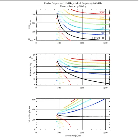
At the next stage, we investigated distortions to the eleva-tion and virtual height patterns caused by an arbitrary phase offset,ΔΨ. In Fig. 5, the unperturbed values (ΔΨ= 0) forfmF2= 9 MHz are plotted by a solid black line, while the

coloured diamonds correspond to different offset values ranging from 0 to 360° in 60° steps. The offset causes some phase values to go outside of the “allowed” range so these values are automatically brought inside the range by either adding or subtracting 2π. As a result, most of the phase curves in Fig. 5 exhibit a 2π discontinuity which shifts to longer ranges with increasing ΔΨ. The general effect on elevation is that the retrieved angle, instead of following a monotonous dependence on range, is split into two seem-ingly unrelated populations. To the left from the phase discontinuity (closer ranges), elevation decreases faster compared to the situation with no offset, while to the right (farther ranges) the situation is the opposite. The most noticeable effect on the virtual height is that at farther ranges, instead of becoming nearly constant, the derived virtual height increases monotonically.

Proposed calibration method

Based on the simulation results, the first step would be to analyse if the experimental elevation-range depen-dences for GS match the expected dependence on range. If they show patterns similar to those in Fig. 5, i.e. with sharp phase jumps and increasing virtual height at larger ranges, then one would need to introduce an extra phase/time offset so that the patterns would look as those in Fig. 4. While this task seems to be simple, there are several critical points to consider.

The most important factor is a correct interpretation of the data uncertainties. Previous studies by Ponomarenko et al. (2011a) have demonstrated that the accuracy of the phase estimates is mainly limited by variations arising from the statistical nature of the radar returns. The same phase fluctuation levels lead to larger elevation errors at lower angles due to the strongly non-linear phase-elevation trans-fer function nearΨmax(Fig. 2). At low elevation levels, the

bulk of measured phase shift values will lie just below the maximum possible value,Ψmax, but the statistical spread in

the measured phase will shift some of the “true” phase values beyondΨmax. The data processing software

automat-ically subtracts 2π from these values to shift them inside the“allowed”phase range so that the adjusted phase values become close to Ψmax−2π, i.e. the respective elevation

values are shifted to the maximum value corresponding to the first 2π“wrap”,Δ2π. As a result, at far ranges (low

eleva-tion), even properly calibrated data should contain some sporadic discontinuities caused by the statistical variability of the phase measurements. However, on the range-time

map, these discontinuities should present just isolated pixels of high elevation values on the predominantly low elevation background.

The above “statistical” discontinuities should not be confused with those observed when echo elevation truly exceeds Δ2π. In contrast with the statistical error in the

phase, the latter are automatically shifted to the lower elevation values. This sort of discontinuity is easy to rec-ognise because it is generally located at closer ranges and represents a regular feature which is observed across

consecutive scans. Most importantly, in this case, there will be no increase in the virtual height at progressively larger ranges.

Based on the above observations, we propose a new method to detect and measure the phase offset using visual analysis of the range-time elevation maps for ground scat-ter. The technique is based on consecutive adjustments of the interferometer phase until the elevation data show the expected pattern, i.e. a general decrease of elevation with range which shows at large distances a near-zero back-ground accompanied by sporadic isolated“jumps”to values close to Δ2π. Conveniently, in the hardware radar profile,

there is a parametertdiffwhich allows for phase adjustment in terms of time delay expressed in nanoseconds. At the time of publication, the Virginia Tech SuperDARN group (2015) provided an opportunity to perform the adjustment procedure by tuningtdiff and visually analysing the result-ing elevation patterns.

Results and discussion

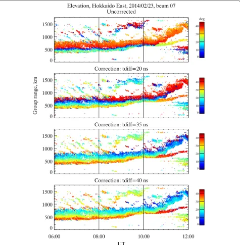
We illustrate the validity and effectiveness of our new calibration method by analysing a 6-h interval (06:00– 12:00UT, 23 February 2014) of the data from Hokkaido East SuperDARN radar as shown in Fig. 6. Here, the top

Fig. 5Same as in Fig. 4 but for the fixed radar frequency of 9-MHz data with varying phase offset

panel shows an uncorrected range-time elevation map for beam 7. In this figure, we used range calculated for GS scatter (defined a half of the group time of flight) so that it roughly corresponds to the ionospheric“reflection”point of the radio wave. Several propagation modes can be identified here: (1) a continuous band of GS covering 400–800 km which starts to move farther away after 9UT; (2) oblique patches of echoes generated by travelling ionospheric disturbances (TIDs) between 800 and 1500 km; (3) a relatively narrow band of ground scatter from the

back-lobe clearly seen after 10:30UT between 600 and 900 km. The latter component has been identified based on the criteria for the back-lobe elevation described in Milan et al. (1997). There are also some other patches of echoes which might be related to either ionospheric scatter (11:30– 12:00UT, 300–600 km) or second-hop ground scatter (9:00–10:00UT, 1200–1500 km).

Here, we focus on the main-lobe GS component for which uncorrected elevation exhibits an abrupt change from very low to very high values at ≈500 km. This

change indeed looks unphysical and therefore attributed to the effect of an unaccounted for time/phase delay in the radar’s hardware.

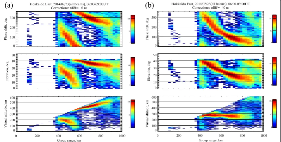
In Fig. 7a, we show statistical analysis of the original (uncorrected) data and present two-dimensional range histograms of the phase (top), elevation (middle) and virtual height (bottom). Adequate statistical analysis requires the analysed dataset to be stationary and we therefore limited the analysed interval to 06:00–09:00UT when the propagation conditions remained essentially constant. Furthermore, in order to increase the number of data points, we included in our analysis data from all 16 beams. Phase was automatically confined to the con-ventional interval corresponding to the elevation values between 0 andΔ2π, as highlighted by red in Fig. 2. While

the elevation and virtual height for the uncorrected data show two apparently independent populations, the phase clearly demonstrates a single population“wrapped” aroundΨ0−2π. By comparing the experimental data with

the simulation from Fig. 4, we identified the presence of a phase offset of≈150°–160°.

The following plots in Fig. 6 show step-by-step correc-tion by applying a gradually increasing time delay (top to bottom). For tdiff= 20 ns, the jump from low to high elevation angles shifts to≈600–650 km. Attdiff= 35 ns, the regular discontinuity virtually disappears, but a close look at the farther edge of the ground scatter band during 10:00–12:00UT reveals that multi-point patches of very high elevation are still observed against the low elevation background. By further increasing the time

delay to 40 ns (bottom), the high elevation patches are reduced to isolated pixels, at which stage we assumed that no more correction is needed.

Figure 7b shows that once the 40-ns correction has been applied, a single population of echoes is present whose elevation monotonically decreases with range and whose virtual height lies near 280 km. The phase shift required to recover a continuous phase population is close to 160° which, in terms of time delay, is close to 40 ns at the Hokkaido East radar operation frequency of

f≈11 MHz. A distinct but relatively small population in the top right corners of the elevation and phase distri-butions represents mainly second-hop echoes, while an-other population at close ranges centred at Δ≈10° results from “wrapping” of the returns whose elevation exceedsΔ2π.

While the graphic representation of the elevation-vs-range dependence in Fig. 7 is more convenient for estimat-ing the bulk phase/time offset, its “fine tuning” is more efficiently performed utilising highly contrasting colours for the low and high elevation values in the range-time maps (Fig. 6).

It shall be noticed that our proposed method allows for estimating the phase offset within a 2πrange so it is gener-ally limited to a single working frequency. As a result, for multi-frequency datasets, the effective time delay (tdiff) has to be determined at each working frequency separately. On the other hand, if for a given radar the phase offset is caused by a frequency-independent time delay, the multi-frequency data would allow to evaluate the actual (i.e.

Fig. 7Two-dimensional histograms of the phase (top), elevation (middle) and virtual height (bottom) vs range calculated for the 06–09UT interval from Fig. 6 but using all radar beams:athe original (uncorrected) data;bdata corrected withtdiff= 40 ns

multi-2π) offset assuming a linear dependence of the phase shift on the radar frequency. For obvious reasons, one has to avoid using data obtained under highly perturbed condi-tions, and datasets related to different hardware and soft-ware updates should be tested separately.

Conclusions

In this work, we have proposed an empirical method to detect and measure phase offsets in HF interferometry data. The proposed method allows for reliable post-calibration of the historic data, i.e. when the conventional calibration using signal generators is frequently too challenging or nearly impossible, e.g. owing to changes in the hardware. The method is based on analysing the progression of eleva-tion angle with range for ground scatter echoes and uses a gradual adjustment of the phase shift until the observed dependence agrees with that expected from a reflecting ionospheric layer. The theoretical basis for this technique was laid through the simulation of ground scatter propaga-tion characteristics using numerical ray tracing and an analysis of the effects of phase fluctuations on elevation. The method was successfully applied to Hokkaido East SuperDARN radar data producing a reliable estimate of the virtual reflection height. The method also provides the basis to extend diagnostic capabilities of the network to a meas-ure of the background electron density (Ponomarenko et al. 2011b). The use of the proposed technique is not limited to SuperDARN and can be applied to any kind of HF interfer-ometry data.

Abbreviations

SuperDARN:Super Dual Auroral Radar Network; HF: high-frequency range of electromagnetic emission (3-30 MHz).

Competing interests

The authors declare that they have no competing interest.

Authors’contributions

The idea of the phase calibration and its implementation belong to PP. NN and JPSM made substantial contributions to establishing the physical basis for the algorithm and clarifying the details of its implementation. AO and TT performed the bulk of analysis of the Hokkaido East data. All authors read and approved the final manuscript. All authors read and approved the final manuscript.

Acknowledgements

We would like to thank all the staff who contributed to the HF radar experiment at Hokkaido. This work was supported by Special Funds for Education and Research (Energy Transport Processes in Geospace) of the Ministry of Education, Culture, Sports, Science and Technology of Japan. This work was supported in part by funding from the Government of Canada for a Canada Research Chair (JPSM).

Author details

1_{Solar-Terrestrial Environment Laboratory, Nagoya University, Nagoya, Japan.} 2

Institute of Solar-Terrestrial Physics, Siberian Branch of the Russian Academy of Sciences, Irkutsk, Russia.3_{University of Saskatchewan, Saskatoon, SK,}

Canada.

Received: 21 March 2015 Accepted: 19 August 2015

References

André D, Sofko GJ, Baker K, MacDougall J (1998) SuperDARN interferometry: meteor echoes and electron densities from ground scatter. J Geophys Res 103:7003–7015. doi:10.1029/97JA02923.

Blanchard GT, S Sundeen S, Baker KB (2009) Probabilistic identification of high-frequency radar backscatter from the ground and ionosphere based on spectral characteristics. Radio Sci 44:RS5012. doi:10.1029/2009RS004141. Chisham G, Lester M, Milan SE, Freeman MP, Bristow WA, Grocott A, McWilliams

KA, Ruohoniemi JM, Yeoman TK, Dyson PL, Greenwald RA, Kikuchi T, Pinnock M, Rash JPS, Sato N, Sofko GJ, Villain J-P, Walker ADM (2007) A decade of the Super Dual Auroral Radar Network (SuperDARN): scientific achievements, new techniques and future directions. Surv Geophys 28:33–109.

doi:10.1007/s10,712-007-9017-8.

Greenwald RA, Baker KB, Dudeney JR, Pinnock M, Jones TB, Thomas EC, Villain J-P, Cerisier J-C, Senior C, Hanuise C, Hunsucker RD, Sofko G, Koehler J, Nielsen E, Pellinen R, Walker ADM, Sato N, Yamagishi H (1995) DARN/SuperDARN: a global view of the dynamics of high‐latitude convection. Space Sci Rev 71:761–795 Kelso JM (1964) Radio ray propagation in the ionosphere. McGraw-Hill, New York Milan SE, Jones TB, Robinson TR, Thomas EC, Yeoman TK (1997) Interferometric

evidence for the observation of ground backscatter originating behind the CUTLASS coherent HF radars. Ann Geophys 15:29–39. doi:10.1007/s00585-997-0029-y.

Ponomarenko PV, St-Maurice J-P, Waters CL, Gillies RG, Koustov AV (2009) Refractive index effects on the scatter volume location and Doppler velocity estimates of ionospheric HF backscatter echoes. Ann Geophys 27:4207–4219. doi:10.5194/angeo-27-4207-2009.

Ponomarenko P, Wiid J, Koustov A, St.-Maurice J-P (2011a) Making sense of SuperDARN elevation: phase offset and variance. In Program and Abstracts for the SuperDARN 2011 Workshop, Thayer School of Engineering, Dartmouth College, Hanover, NH, US, 29 May-03 June 2011

Ponomarenko PV, Koustov AV, St.-Maurice J-P, Wiid J (2011b) Monitoring the F-region peak electron density using HF backscatter interferometry. Geophys Res Lett. doi:10.1029/2011GL049675.

Ruohoniemi JM, Baker KB (1998) Large‐scale imaging of high-latitude convection with Super Dual Auroral Radar Network HF radar observations. J Geophys Res 103:20,797–20,811

Virginia Tech SuperDARN group (2015). Range-time plotting on-line tool. http:// vt.superdarn.org/tiki-index.php?page=DaViT+RTP. Accessed on 28 August 2015

Submit your manuscript to a

journal and benefi t from:

7Convenient online submission 7Rigorous peer review

7Immediate publication on acceptance 7Open access: articles freely available online 7High visibility within the fi eld

7Retaining the copyright to your article