R E S E A R C H
Open Access
Statistical analysis of inter-cell interference in
uplink OFDMA networks with soft frequency
reuse
Yuanping Zhu
1,3, Jing Xu
1,2*, Jiang Wang
1,2and Yang Yang
1,2Abstract
As the inter-cell interference becomes a great challenge in frequency reuse one systems, soft frequency reuse (SFR) has been widely used to deal with the severe inter-cell interference especially for cell edge users. This paper proposes an analytical method to investigate the statistics of inter-cell interference in uplink orthogonal frequency division multiple access systems when SFR scheme is adopted. Probability density functions of inter-cell interference in different frequency bands are derived and then used to deduce the expectation and variance of inter-cell interference from multiple interfering cells. The derivations are validated through numerical results. In addition, the relationship between system parameters and the statistics of inter-cell interference in different frequency bands is investigated. These contributions will give insights and guidelines for the system optimization.
1 Introduction
Orthogonal frequency division multiple access (OFDMA) has been adopted in many wireless networks such as IEEE 802.16 and the 3rd Generation Partnership Project long-term evolution (LTE), due to many beneficial char-acteristics. Meanwhile, as the limited frequency resource becomes a bottleneck for the increasing data rate demand, it would be better to reuse the available frequency among each cell. However, inter-cell interference (ICI) will be more severe for user equipments (UEs) in the cell edge region. Many inter-cell interference coordination (ICIC) techniques have been proposed to mitigate the problem. One typical solution introduced in LTE [1] is soft fre-quency reuse (SFR): (1) UEs in the cell center region which experience/generate low interference and require low power to communicate with their serving evolved NodeBs (eNBs) are permitted to use the whole spectrum, and (2) UEs in the cell edge region which experience/generate strong interference and require high power to ensure reli-able communication are constrained to be scheduled with
*Correspondence: [email protected]
1Key Laboratory of Wireless Sensor Network & Communication, Shanghai Institute of Microsystem Information and Technology (SIMIT), Chinese Academy of Sciences (CAS), Shanghai 200050, People’s Republic of China 2Shanghai Research Center for Wireless Communications (WiCO), Shanghai 200335, People’s Republic of China
Full list of author information is available at the end of the article
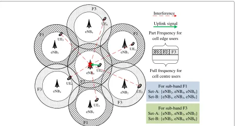
a part of the spectrum, while these resources should be allocated to UEs in the center region or not be used in neighboring cells. With such resource scheduling limita-tion among adjacent cells, SFR can be utilized to avoid severe ICI. Figure 1 demonstrates an example of the SFR scheme for multicell cellular networks.
If statistical characteristics of ICI can be derived through theoretical analysis, time-consuming system-level simulations may be avoided. Therefore, researches about statistics of ICI have received more and more consideration recently. Some of them focus on analyz-ing the statistics of to-interference ratio or signal-to-interference-and-noise ratio (SINR) analytically [2-6]. Others concern the probability density function (PDF) of ICI or SINR. The conditional PDF of carrier-based interference plus noise in downlink OFDMA networks is derived in [7]. In [8,9], the PDFs of SINR and interference are derived through analyzing the samples of system-level simulations and checking several given hypotheses, without deriving and validating the corresponding closed-form expressions. In [10], the PDF of downlink SINR in randomly located femtocells is given by analysis and calculation. Recently, many analytical frameworks are pre-sented to evaluate the distribution of downlink SINR based on the Poisson point process modeling of nodes [11,12]. These papers focus on the statistical analysis of the downlink ICI in cellular networks.
eNB1
eNB2
eNB3 eNB4
eNB5
eNB6
UE4
UE3 UE5
UE6
UE1
UE2
Interference
Uplink signal
F1 F2 F3
Full frequency for cell centre users Part Frequency for
cell edge users
For sub-band F1 Set-A: {eNB2, eNB4, eNB6} Set-B: {eNB1, eNB3, eNB5}
For sub-band F3 Set-A: {eNB1, eNB3, eNB5} Set-B: {eNB2, eNB4, eNB6} eNB0
UE0
F2
F3 F3
F1
F1 F1
F3
Figure 1Uplink interference model when SFR is adopted in cellular networks.
It is worth noting that in the downlink, the sources of interference are eNBs which are fixed in cellular networks, thus the scheduling scheme almost has no impact on the ICI once the frequency reuse scheme is determined. How-ever, the uplink interfering sources are UEs which may be located anywhere in a cell. Moreover, in different schedul-ing periods, an uplink frequency band may be allocated to different UEs. As a result, the uplink interference will show great fluctuation, and the analysis of the down-link interference cannot be applied to analyze the updown-link interference directly. In [13], the PDF of SINR inad hoc networks is derived. Only one interferer is considered in this scenario, and the derived results may not be applied to cellular networks. The uplink ICI is investigated in [14] by generating amounts of samples and then drawing a his-togram without deriving a closed-form expression. The uplink coverage probability in cellular networks is derived in [15] when the power control scheme is involved, and all the nodes are assumed to be randomly placed.
In this paper, the fixed infrastructure and randomly dis-tributed UEs are considered in the model of cellular net-works with SFR scheme. And for the channel model, the path loss, shadowing, and Rayleigh fading are included. Based on such system assumptions, the PDFs of ICI in dif-ferent frequency bands are derived and used to deduce the closed-form expressions for the expectation and vari-ance. Furthermore, the impacts of many system param-eters on the PDF, expectation, and variance of ICI are investigated.
The rest of the paper is organized as follows. Section 2 introduces the system model. The PDF, expectation, and variance of the uplink ICI in the frequency band allo-cated to cell edge UEs in the cell of interest are derived in section 3. And the corresponding statistical analysis of the uplink ICI in the rest frequency bands are given in section 4. In section 5, the numerical results are demon-strated, and the influences of system parameters on the uplink ICI are studied. Finally, conclusions are made in section 6.
2 System model
Considering that in the actual deployment of cellular net-works, the infrastructures are always fixed while UEs are randomly distributed, and the propagation attenuation is related to the distance. It is rational to model the cov-erage area of a cell as a circular region. For simplicity, the model of cellular network consists of a cell of inter-est and its neighboring cells as depicted in Figure 1; the serving eNB in the cell of interest is defined as eNB0,
For the SFR scheme, the whole frequency band is divided into three sub-bands: F1, F2, and F3 as shown in Figure 1. Exterior UEs are constrained to use one of the sub-bands with high transmit powerPt,1, while the
interior UEs can reuse the whole frequency band with a reduced powerPt,0(Pt,0<Pt,1). In this paper,Pt,1is set as
the full transmit power. UEs are assumed to be uniformly distributed in the cellular networks, and all the frequency bands are allocated to active UEs in every cell. In addition, eNB schedule frequency resources independently under the premise of allocating orthogonal sub-bands to cell edge UEs among adjacent cells.
In uplink, eNB0 receives the desired signal from UE0
and interference from UEs in the neighboring cells. The signal link is represented by green solid arrow while the interference links are represented by red dashed arrows in Figure 1.
For the channel model, the distance-dependent path loss, shadowing, and Rayleigh fading are considered. These three parts are independent. The shadowing is modeled as a lognormal random variable (RV), and the gain related to Rayleigh fading is modeled as an exponential-distributed RV. Besides, we assume that the antenna pattern of both UEs and eNBs are omnidirec-tional. Therefore, the uplink interference power from UEi can be described as
Ii=PtαD−i βeλξH (1)
where Ii indicates the received interference at eNB0, Pt
denotes the transmit power of UEiwhich equals to either Pt,0orPt,1,Direpresents the distance between eNB0and
UEi, α and β are the path loss constant and exponent,
respectively,αD−iβ represents the path loss,ξ represents the logarithmic shadowing in the unit of dB which is assumed to be a zero-mean Gaussian RV with varianceσ2, λ = ln(10) /10, andHrepresents the gain related to the Rayleigh fading.
As the SFR scheme is adopted, the distribution of inter-ference in sub-bands F2 and F1/F3 (we define F1/F3 which represents ‘F1 or F3’ for convenience) will be different. In the following, they will be analyzed separately.
3 Statistical analysis of the uplink ICI in sub-band F2
Since the neighboring cells have identical relative loca-tions to the cell of interest, it would be tractable to analyze the interference from one interfering cell at first and then extend to the multiple interfering cells’ scenario.
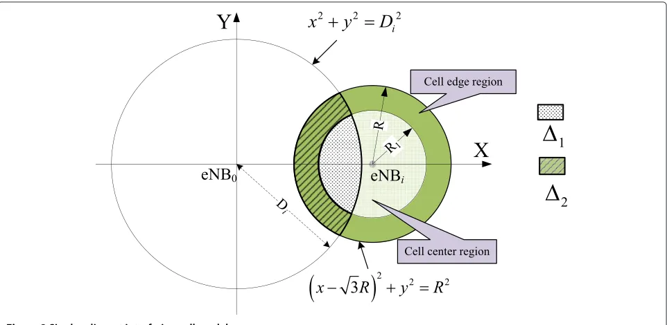
As shown in Figure 2, the cell radius is R, and the intersite distance is √3R; eNB0 is located at the
origi-nal point (0,0), and eNBi is located at ( √
3R, 0). In the interfering cell, the inner disk represents the cell center region, the green annular area represents the cell edge region, andR1 = γR(0 ≤ γ ≤ 1) indicates the radius
of the cell center region. The overlapping area between the cell center region of the interfering cell and the cir-cular region x2+ y2 ≤ D2i is defined as 1, while 2
denotes the overlapping area between the cell edge region of the interfering cell and the circular regionx2+y2 ≤ D2i.
DefineX=eλξ,Y=αD−β
i , and suppose that the trans-mit power of UE is given, the random part ofIiisXYH,
whereX,Y, andHare independent. The PDF of the prod-Y, andHare obtained.
The distribution of the shadowingξis modeled as zero-mean Gaussian distribution which is denoted asN(0,σ2), thus, the PDF ofX=eλξcan be derived as
SinceHrepresents the power gain of Rayleigh fading, the PDF ofHis modeled as
fH(h)=μe−μh,h>0 (4)
where μ is the rate parameter and is always set as 1 traditionally.
3.1 PDF of the ICI in sub-band F2
For convenience, we define Lcenter represents the event
that UEi locates in the cell center region and Ledge
rep-resents the event that UEi locates in the cell edge region. From Figure 1, it is obvious that the received interfer-ence at eNB0 in sub-band F2 comes from the interior
UEs of the neighboring cells, which means that the event Lcenter occurs. Therefore, from Figure 2, the conditional
cumulative distribution function (CDF) of Di equals to the proportion of the area of1to the area of cell center
region. That is conditional PDF of Diequals to the first derivative of CDF, and it is given by
Based on (7), it is easy to derive the conditional PDF of the path lossY =αD−i βas conditional PDF ofYis
fY
The interference from the interior UEs in a neighboring cell isIi=Pt,0XYH, and its PDF is derived as
Suppose that N represents the number of
neighbor-ing cells, IF2 =
N
i=1
Ii is the total received
interfer-ence in sub-band F2 from multiple neighboring cells. As mentioned in section 2, each cell schedule fre-quency resources independently. This indicates that in sub-band F2, the ICI from the different neighboring cells are independent and identically distributed (i.i.d.) random variables. With the PDF of the ICI from sin-gle neighboring cell, the PDF of IF2 is calculated by
the Nth order convolution of (10) as shown in (11), where ‘ * ’ represents the convolution. The convolution can be calculated using numerical calculation methods.
fIF2 =fIi(I|Lcenter)∗ · · · ∗ fIi(I|Lcenter) N−th order convolution
(11)
3.2 Expectation and variance of the uplink ICI in sub-band F2
Since the shadowingX, path lossY, and Rayleigh fad-ing H are independent, themth moment of Ii could be calculated as
E(Ii)m=E(PtXYH)m=(Pt)mEXmEYmEHm
(12)
where E[()m] represents themth moment of the corre-sponding RV.
To get closed-form expressions for the moments ofY , we use the power series of arccosine function to derive an instituted expression of fYyLcenter.The instituted
expression is
Similarly, the conditionalmth moment ofYcan be calcu-lated as
For the lognormal shadowing X, the expectation is
E[X]=
For the Rayleigh fadingH, themth moment is
E[Hm]=
∞
0
hmμe−μhdh= m!
μm (22)
Hence, it is easy to derive the expectation ofIias
E[Ii|Lcenter]=Pt,0E[X]E[Y|Lcenter]E[H]
= Pt,0αM0(β,γ )
μγ2Rβ e λ2σ2
2 (23)
Then, the conditional variance ofIiis given by
As the interference in sub-band F2 from neighboring cells are i.i.d. RVs, the expectation and variance of IF2 are
shown as:
Considering thatα,β, andμare constants, the two statis-tics ofIF2are affected byR,Pt,0,γ, andσ. Intuitively, the
expectation ofIF2 is proportional toPt,0,R−β, ande
λ2σ2
2 ,
while the variance ofIF2is proportional toPt,02 andR−2β.
The influence of γ andσ on the expectation and vari-ance ofIF2 will be investigated through numerical results
in section 5.
4 Statistical analysis of the uplink ICI in sub-band F1/F3
In this case, the interfering cells need to be differentiated into two classes, due to different distributing scenarios of interfering sources. In order to describe the two classes, here we choose the ICI in sub-band F1 as an example. From Figure 1, in the cells served by eNB2, eNB4, and
eNB6, the sub-band F1 will be allocated to only the
inte-rior UEs. Differently, eNB1, eNB3, and eNB5can allocate
sub-band F1 to all the connected UEs. For convenience, we define the cluster of interfering cells which can allocate the given sub-band to only the interior UEs as Set-A, and the cluster of interfering cells which can allocate the given sub-band to all the connected UEs as Set-B. Similarly, in sub-band F3, the neighboring cells will be divided into the two classes also. In Figure 1, the Set-A and Set-B for both sub-band F1 and F3 are presented.
4.1 PDF of the uplink ICI in sub-band F1/F3
For both the transmitting power and the path loss depend on the location of interfering UEs, the distribution of interference from the cells of Set-A and the cells of Set-B should be analyzed separately.
For the scenario that interfering UEs are in the cells of Set-A, the corresponding PDF of Ii is fI(Set−A)
i (I) =
fIi(I|Lcenter). In the cells of Set-B, the interfering UEs
locate in either the cell center region or the cell edge region. Define the product ofPtandY = αD−i β asK = PtY. The distribution function ofKcan be expressed as
PSet−B(k<K)=P(Lcenter,k<K)+P(Ledge,k<K)
(28)
As we know, the joint distribution functions shown in (28) can be calculated by
P(Lcenter,k<K)=P(Lcenter)P(k<K|Lcenter)
P(Ledge,k<K)=P(Ledge)P(k<K|Ledge)
(29)
Apparently, the probability of interfering UE being located in the cell center region is P(Lcenter) = γ2, and the
probability of it being located in the cell edge region is P(Ledge) = 1−γ2. Hence, the PDF ofK can be derived
From Figure 2, if the event Ledgeoccurs, the conditional
CDF ofDiequals the ratio between the area of2and the
area of cell edge region. That is
Fd(Di|Ledge)=
S1represents the overlapping area between the circular
regionx2+y2 ≤ D2
fd(Di|Ledge)=
Then, the conditional PDF of Di when Ledge occurs can
be derived through the first derivative ofFd(Di|Ledge). It is
given by
where the two distribution ranges ofDiare given by1=
(√3−1)R,(√3−γ )R!∪ (√3+γ )R,(√3+1)R, and 2=(√3−γ )R,(√3+γ )R.
Then, the conditional PDF of the path lossY can be derived as
Consequently, we could get that
fY(y|Ledge)=F1y−2/β−1
be obtained. Then, for the scenario that interfering UEs are in the cells of Set-B, the PDF ofIicould be derived as
fI(Set−B)
Suppose thatMrepresents the number of cells in Set-A, andQrepresents the number of cells in Set-B. The total
interference in sub-band F1/F3 isIF1/F3 =
M
can be calculated by(M+Q)-th order convolution as
fIF1/F3 =fIi(Set−A)∗ · · · ∗fI(iSet−A)
M−th order convolution
∗fI(Set−B)
i ∗ · · · ∗fI
(Set−B)
i
Q−th order convolution
(38)
Similar to (11), the PDF of the total ICI in sub-band F1/F3 shown in (38) can be derived using numerical cal-culation methods.
4.2 Expectation and variance of the uplink ICI in sub-band F1/F3
Based on the previous analysis, it is known that the expec-tation and variance of interference from one cell in Set-A are the same as the expressions presented in (23) and (25), respectively. Therefore, the expectation and variance of ICI from a cell in Set-B should be calculated to deduce the two statistics of total ICI in sub-band F1/F3.
Using the same method of power series and polynomial expansion which has been used to derive the substituted expression offY
yLcenter
in subsection 3.2, we could get that
Furthermore, when Ledgeoccurs, them-th moment ofYis
given by
E[YmLedge]=
αM1(mβ) −αM0(mβ,γ )
Then, the expectation of interference from a cell in Set-B can be calculated as
E[Ii(Set−B)]=E[K(Set−B)]E[X]E[H]
=#P(Lcenter)Pt,0E[Y|Lcenter]
+P(Ledge)Pt,1E[YLedge]
$
E[X]E[H]
= Pt,1αM1(β)+(Pt,0−Pt,1)αM0(β,γ )
μRβ e
λ2σ2
2
(45)
Moreover, themth moment of interference from one cell of Set-B is
E[ Ii(Set−B) !m
]
=(Pt,1α)mM1(mβ)+(Pt,0m−Pmt,1)αmM0(mβ,γ )
μmRmβ m!e
m2λ2σ2
2
(46)
With (45) and (46), the variation of interference from one cell in Set-B can be calculated as
V arSet−B[Ii]=
α2e2λ2σ2 μ2R2β 2
P2t,1M1(2β)
+(Pt,02 −P2t,1)M0(2β,γ )
−α2eλ
2σ2
μ2R2β
Pt,1M1(β)
+(Pt,0−Pt,1)M0(β,γ )
2
(47)
Using the corresponding statistics of interference from one cell of Set-A and Set-B, the expectation and variance
of total interferenceIF1/F3=
M
i=1
Ii(Set−A)+ Q
i=1
Ii(Set−B)are
E[IF1/F3]=
M
i=1
ESet−A[Ii]+ Q
i=1
ESet−B[Ii]
= MPt,0αM0(β,γ )
μγ2Rβ e λ2σ2
2
+ Pt,1αM1(β)+(Pt,0−Pt,1)αM0(β,γ )
μRβ Qe
λ2σ2
2
(48)
V ar[IF1/F3]=
M
i=1
VarSet−A[Ii]+ Q
i=1
VarSet−B[Ii]
=M(Pt,0α)2eλ
2σ2
μ2γ2R2β
2M0(2β,γ )eλ
2σ2
−[M0(β,γ )]2
γ2
+ 2Qα2e2λ
2σ2
μ2R2β
P2t,1M1(2β)
(49)
+(P2t,0−P2t,1)M0(2β,γ )
− Qα2eλ
2σ2
μ2R2β
Pt,1M1(β)
+(Pt,0−Pt,1)M0(β,γ )
2
−120 −115 −110 −105 −100 −95 −90 0
0.02 0.04 0.06 0.08 0.1 0.12
ICI(dBm) (σ =4dB, P
t,0=20dBm)
IF2, γ =0.7 IF1/F3, γ =0.7 IF2, γ =0.9 IF1/F3, γ =0.9
γ =0.7
γ =0.7
γ =0.9
γ =0.9
Table 1 System parameters
Parameter Assumption
Cell radiusR 1,000 m
Transmit power of interior UEs Pt,0= 17, 20 dBm
Transmit power of exterior UEs Pt,1= 23 dBm
Antenna pattern of UE and eNB Omnidirectional Antenna gain of UE and eNB 0 dBi
Path loss model 15.3+37.6 log10d, (din m, dB) orα=0.03,β=3.76 Number of neighboring cells N=6
Number of cells in Set-A M=3
Number of cells in Set-B K=3
γ 0.7, 0.9
Standard deviation of shadowing σ= 4, 6 dB
Rate of Rayleigh fading μ= 1
The derived expressions shown in (48) and (49) are more complicated than the corresponding statistics ofIF2due to
the SFR scheme. Similar toIF2, the expectation ofIF1/F3is
proportional toR−βandeλ22σ2, and the variance ofI
F1/F3is
proportional toR−2β. The impacts ofγ,P
t,0, andσon the
PDF, expectation, and variance of ICI will be investigated through numerical results in the next section.
5 Analytical and numerical results
In this section, the impact of system parameters (γ,Pt,0,
andσ) on the PDF and statistics of ICI will be investi-gated. Furthermore, the theoretical results are compared
with Monte Carlo simulations to validate the derivations of statistics.
5.1 Impact ofγ on the distribution of ICI.
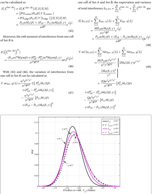
As shown in Figure 3, the theoretical PDF ofIF2andIF1/F3
with two different values ofγ (γ = 0.7,0.9) are presented. The corresponding system parameters are presented in Table 1.
Through the comparison between PDF ofIF2andIF1/F3
with sameγ, it is obvious that the distribution ofIF2
con-centrates on a relatively low level, while the range ofIF1/F3
is wider in the high interference region. That is because some exterior UEs which are scheduled with sub-band F1/F3 in cells of Set-B may generate severe interference. This difference validates the advantage of SFR scheme on decreasing ICI for exterior UEs. Furthermore, the vary-ing ofγ has different influence on the distribution ofIF2
and IF1/F3. Concretely, the distribution of IF2 becomes
more dispersed, and the probability of high interference increases obviously with the increase ofγ. Because the distribution region for the interior UEs is extended, some interfering UEs will be closer to the cell of interest, and some will be further away. However, the distribution of IF1/F3tends to move to the low interference region slowly
asγ increases. For the cells of Set-A, the increase ofγ has the same effect on the distribution of ICI asIF2. Whereas,
increasingγ will reduce the cell edge region for cells of Set-B. Considering that the dominating interfering source of IF1/F3 are the neighboring exterior UEs, the increase
ofγ will result in lower probability for high interference.
−1250 −120 −115 −110 −105 −100 −95 −90 −85 0.02
0.04 0.06 0.08 0.1 0.12
ICI(dBm) (σ =4dB, γ =0.7)
I
F2, Pt,0=20dBm
IF1/F3, Pt,0=20dBm IF2, Pt,0=17dBm I
F1/F3, Pt,0=17dBm
Pt,0=17dBm
Pt,0=20dBm
Table 2 Settings ofPt,0,σ, andγ
Parameter Assumption
Transmitting power and standard deviation of shadowing
case 1:Pt,0= 20 dBm,σ= 4 dB
case 2:Pt,0= 17 dBm,σ= 4 dB
case 3:Pt,0= 20 dBm,σ= 6 dB
γ 0.3, 0.4, 0.5, 0.6, 0.7, 0.8, 0.9, 1
But the tendency of decreasing is not obvious due to the two opposite effects for the different sets of cells (Set-A, Set-B).
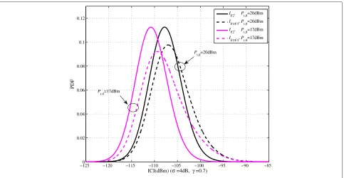
5.2 Impact ofPt,0on the distribution of ICI
The PDF curves ofIF2 andIF1/F3 with different values of
Pt,0(Pt,0= 17, 20 dBm) are demonstrated in Figure 4. For
IF2is proportional toPt,0, the PDF curves ofIF2moves to
the higher interference region without any change of the shape with the increase ofPt,0. Similarly, the PDF ofIF1/F3
near the lower bound moves to the higher interference region with the increase of Pt,0 because the weak
inter-ference ofIF1/F3is mainly determined by the neighboring
interior UEs and is proportional toPt,0. However, the
dis-tribution near the upper bound keeps unchanged for the high interference in sub-band F1/F3 is mainly determined by some neighboring exterior UEs. As a result, the distri-bution of IF1/F3 becomes more concentrated in the high
interference region with the increase ofPt,0.
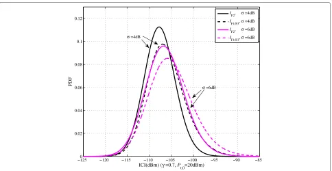
5.3 Impact ofσon the distribution of ICI
To investigate the influence of the shadowing on the dis-tribution of ICI, the standard deviation of shadowing is set
as 4dB or 6dB according typical settings of macro model [16]. As depicted in Figure 5, both the distribution ofIF2
andIF1/F3are influenced by the shadowing greatly. As the
increase ofσ, the distribution of the ICI in both sub-bands becomes more dispersive. The reason is straightforward: large standard deviation of shadowing means the vari-ability of shadowing is great, and it will result in great variability of the received signal or interference.
5.4 Impact of system parameters on the statistics of ICI In this part, the statistics of ICI with different system parameters (γ, Pt,0, and σ) are compared, and Monte
Carlo simulation results are presented to validate the derived expressions of the expectation and variance. Without loss of generality, the standard deviation of ICI is investigated instead of the variance. In addition, it needs to be mentioned that the truncated series of M0(β,γ ),
M0(2β,γ ), M1(β), and M1(2β) are calculated with the
highest order n = 30 to get the theoretical calculation results. The settings ofγ,Pt,0, andσare shown in Table 2.
The expectation and standard deviation of ICI with dif-ferent system parameters are depicted in Figure 6 and Figure 7, respectively. The coincidence between theoreti-cal theoreti-calculations and Monte Carlo simulations validates the derivations on the statistics of ICI. Particularly, γ = 1 means that all cells reuse the whole frequency resources completely. Therefore, the expectation/standard deviation of different sub-bands are same whenγ =1.
From Figure 6, the expectation of IF2 is smaller than
the expectation ofIF1/F3 whenγ < 1. Besides that, asγ
−1250 −120 −115 −110 −105 −100 −95 −90 −85 0.02
0.04 0.06 0.08 0.1 0.12
ICI(dBm) (γ =0.7, P
t,0=20dBm)
I
F2, σ =4dB
I
F1/F3, σ =4dB
IF2, σ =6dB IF1/F3, σ =6dB
σ =4dB
σ =6dB
0.2 0.3 0.4 0.5 0.6 0.7 0.8 0.9 1 −111
−110 −109 −108 −107 −106 −105 −104 −103 −102 −101
γ
Expectation (dBm)
simulation IF2
calculation IF2
simulation IF1/F3
calculation I
F1/F3
Pt,0=20dBm, σ =6dB
Pt,0=20dBm, σ =4dB
Pt,0=17dBm, σ =4dB
Figure 6Expectation of ICI.
increases, the expectation ofIF2 tends to increase
obvi-ously, but the expectation ofIF1/F3will decrease slowly. In
addition, ifPt,0 is reduced, the expectation ofIF1/F3 will
decline faster asγ increases. The reason is that the influ-ence ofPt,0onIF1/F3will be more significant if the interior
UEs occupy larger quantity in the interfering sources. Differently, the expectation ofIF2 is proportional toPt,0.
Furthermore, as the shadowing and the path loss are inde-pendent, it is observed that larger σ will result in the increase of the expectation ofIF2andIF1/F3with the same
margin regardless ofγ.
Figure 7 presents the standard deviation curves of IF2
andIF1/F3. With the given system parameters, the
stan-dard deviation ofIF2is smaller than the standard deviation
0.2 0.3 0.4 0.5 0.6 0.7 0.8 0.9 1
−112 −110 −108 −106 −104 −102 −100 −98 −96
γ
Standard deviation (dB)
simulation IF2
calculation IF2
simulation IF1/F3
calculation IF1/F3
P
t,0=20dBm, σ =6dB
Pt,0=20dBm, σ =4dB
P
t,0=17dBm, σ =4dB
of IF1/F3. This demonstrates the higher fluctuation of
IF1/F3 , which results from the more flexible scheduling
in the cells of Set-B. It needs to be noted that flexible scheduling may result in more diversity gain, but the high fluctuation of ICI will restrict the efficiency of link adap-tive technology. Thus, the variance of ICI is important for the system performance evaluation.
Besides that, the standard deviation ofIF2 increases as
γ for the large cell center region will disperse IF2 in a
wider distribution range. Furthermore, the standard devi-ation of IF2 is proportional toPt,0. However, for IF1/F3,
the standard deviation almost retain the same value if γ < 0.8. Only when γ approaches to 1, the decrease of Pt,0 or the increase of γ will result in the decline of
the standard deviation of IF1/F3. Briefly, the effects of
γ and Pt,0 on the standard deviation of IF1/F3 become
significant only when γ is large enough. The reason is that the exterior UEs produce predominant fluctuation of IF1/F3 generally, but if γ approaches to 1, few
schedul-ing will involve the exterior UEs, then IF1/F3 will mainly
depend on the interior UEs of neighboring cells. In addi-tion, the standard deviation of bothIF2andIF1/F3increase
as σ, and the margin of increase only depends on the shadowing.
6 Conclusions
This paper investigates the statistical model of uplink ICI for OFDMA networks with SFR scheme. Through analyzing the distribution of the path loss, shadowing, and Rayleigh fading, the distributions of ICI in different sub-bands are analyzed separately. Then, the closed-form expressions of the expectation and variance of ICI are derived through the method of power series expansion and validated by Monte Carlo simulations. Based on the numerical results, the impacts of system parameters on the PDF and statistics of ICI in different sub-bands are demonstrated. Concretely, for the sub-band scheduled to the exterior UEs in the cell of interest, the varying ofγ andPt,0has a significant effect on the distribution of ICI.
For the rest frequency bands, the distribution range of ICI is wider, and the expectation and variance of ICI are much higher; the influence ofγ andPt,0on the
expecta-tion of ICI will be significant only when the interior UEs dominate most proportion of interfering sources. Besides that, the standard deviation of shadowing shows a great influence on the distribution of ICI. These derived results can provide guidelines to the design of ICIC scheme parameters and the system performance optimization.
Competing interests
The authors declare that they have no competing interests.
Acknowledgements
This work is sponsored by the National Nature Science Foundation of China under grant 61210002 and the International S&T Cooperation Program of China under grants 2010DFB10410 and 2012DFG11910.
Author details
1Key Laboratory of Wireless Sensor Network & Communication, Shanghai Institute of Microsystem Information and Technology (SIMIT), Chinese Academy of Sciences (CAS), Shanghai 200050, People’s Republic of China. 2Shanghai Research Center for Wireless Communications (WiCO), Shanghai 200335, People’s Republic of China.3University of Chinese Academy of Sciences, Beijing 100049, People’s Republic of China.
Received: 6 June 2012 Accepted: 3 April 2013 Published: 1 May 2013
References
1. Ericsson, inTSG RAN WG1 meeting 42. Inter-cell interference handling for E-UTRA, 3GPP R1-050764 (3GPP London, 2005), pp. 1–4
2. F Graziosi, F Santucci, inProceedings of IEEE Vehicular Technology Conference (VTC). Analysis of second order statistics of the SIR in cellular mobile networks (IEEE Amsterdam, 1999), pp. 1316–1320
3. F Graziosi, L Fuciarelli, F Santucci, inProceedings of IEEE Vehicular Technology Conference (VTC). Second order statistics of the SIR for cellular mobile networks in the presence of correlated co-channel interferers (IEEE Rhodes, 2001 ), pp. 2499–2503
4. F Graziosi, F Santucci, inProceedings of IEEE International Conference on Communications (ICC). On SIR fade statistics in rayleigh-lognormal channels (IEEE New York, 2002), pp. 1352–1357
5. FA Ramos, V Ya Kontorovitch, M Lara, inProceedings of IEEE Vehicular Technology Conference (VTC). On the second order statistics of SIR in wireless Nakagami channels (IEEE Orlando, 2003), pp. 3131–3135 6. KA Hamdi, On the statistics of signal-to-interference plus noise ratio in
wireless communications. IEEE Trans. Commun.57(11), 3199–3204 (2009) 7. C Seol, K Cheun, A statistical inter-cell interference model for downlink
cellular OFDMA networks under log-normal shadowing and multipath rayleigh fading. IEEE Trans. Commun.57(10), 3069–3077 (2009) 8. SN Moiseev, SA Filin, MS Kondakov, AV Garmonov, DH Yim, J Lee, S
Chang, YS Park, inProceedings of IEEE International Conference on Communications (ICC). Analysis of the statistical properties of the SINR in the IEEE 802.16 OFDMA network (IEEE Istanbul, 2006), pp. 5595–5599 9. SN Moiseev, SA Filin, MS Kondakov, AV Garmonov, DH Yim, J Lee, S Chang,
YS Park, inProceedings of IEEE Wireless Communications and Networking Conference (WCNC). Analysis of the statistical properties of the interference in the IEEE 802.16 OFDMA network (IEEE Las Vegas, 2006), pp. 1830–1835 10. KW Sung, H Haas, S McLaughlin, A semianalytical PDF of downlink SINR
for femtocell networks. EURASIP J. Wireless Commun. Netw. 2010, 9 (2010)
11. TD Novlan, RK Ganti, A Ghosh, JG Andrews, Analytical evaluation of fractional frequency reuse for OFDMA cellular networks. IEEE Trans. on Wireless Commun.10(12), 4294–4305 (2011)
12. S Mukherjee, Distribution of downlink SINR in heterogeneous cellular networks. IEEE J. Selected Areas Commun.30(3), 575–585 (2012) 13. A Musesir, M Bode, KW Sung, H Haas, Analysis SIR for self-organizing
wireless networks. EURASIP J. Wireless Commun. Netw.2009, 8 (2009) 14. I Viering, A Klein, M Ivrlac, M Castaneda, JA Nossek, inProceedings of IEEE
International Conference on Communications (ICC). On uplink intercell interference in a cellular system (IEEE Istanbul, 2006), pp. 2095–2100 15. TD Novlan, HS Dhillon, JG Andrews, Analytical modeling of uplink cellular
networks . http://arxiv.org/abs/1203.1304 Accessed 15 Mar 2012 16. 3GPP TR 36.814 v9.0.0. Further advancements for E-UTRA physical layer
aspects, (2010)
doi:10.1186/1687-6180-2013-96