Volume 2006, Article ID 74812, Pages1–14 DOI 10.1155/WCN/2006/74812
Error Control Coding in Low-Power Wireless Sensor Networks:
When Is ECC Energy-Efficient?
Sheryl L. Howard, Christian Schlegel, and Kris Iniewski
Department of Electrical&Computer Engineering, University of Alberta, Edmonton, AB, Canada T6G 2V4
Received 31 October 2005; Revised 10 March 2006; Accepted 21 March 2006
This paper examines error control coding (ECC) use in wireless sensor networks (WSNs) to determine the energy efficiency of specific ECC implementations in WSNs. ECC provides coding gain, resulting in transmitter energy savings, at the cost of added decoder power consumption. This paper derives an expression for the critical distancedCR, the distance at which the decoder’s energy consumption per bit equals the transmit energy savings per bit due to coding gain, compared to an uncoded system. Re-sults for several decoder implementations, both analog and digital, are presented fordCR in different environments over a wide frequency range. In free space,dCRis very large at lower frequencies, suitable only for widely spaced outdoor sensors. In crowded environments and office buildings,dCRdrops significantly, to 3 m or greater at 10 GHz. Interference is not considered; it would lowerdCR. Analog decoders are shown to be the most energy-efficient decoders in this study.
Copyright © 2006 Sheryl L. Howard et al. This is an open access article distributed under the Creative Commons Attribution License, which permits unrestricted use, distribution, and reproduction in any medium, provided the original work is properly cited.
1. INTRODUCTION
Wireless sensor networks are currently being considered for many communications applications, including industrial, se-curity surveillance, medical, environment and weather mon-itoring, among others. Due to limited embedded battery life-time at each sensor node, minimizing power consumption in the sensors and processors is crucial to successful and re-liable network operation. Power and energy efficiency is of paramount interest, and the optimal WSN design should consume the minimum amount of power needed to pro-vide reliable communication. New approaches in transmitter and system design have been proposed to lower the required power in the sensor network [1–14].
Error control coding (ECC) is a classic approach used to increase link reliability and lower the required transmitted power. However, lowered power at the transmitter comes at the cost of extra power consumption due to the decoder at the receiver. Stronger codes provide better performance with lower power requirements, but have more complex decoders with higher power consumption than simpler error control codes. If the extra power consumption at the decoder out-weighs the transmitted power savings due to using ECC, then ECC would not be energy-efficient compared with an un-coded system.
Previous research using ECC in wireless sensor networks focused primarily on longtime industry-standard codes such
as Reed-Solomon and convolutional codes. A hybrid scheme choosing the most energy-efficient combination of ECC and ARQ is considered in [15], using checksums, CRCs, Reed-Solomon and convolutional codes. A predictive error-correction algorithm is presented in [16] which uses data correlation, but is not an error control code, as there is no encoding. Power-aware, system-level techniques including modulation and MAC protocals, as well as differing rate and constraint length convolutional coding, are considered in [17] to reduce system energy consumption in wireless mi-crosensor networks. Depending on the required bit error rate (BER), a higher rate convolutional code, or no coding at all, could be the most energy-efficient approach.
This paper examines several different decoder implemen-tations for a range of ECC types, including block codes, convolutional codes, and iteratively decoded codes such as turbo codes [18] and low-density parity-check codes (LD-PCs) [19]. Both digital and analog implementations are con-sidered. Analog implementations seem a natural choice for low-power applications due to their minimal power con-sumption with subthreshold operation.
[20,21] is extended to a more realistic power consumption model, and transmitter efficiency is considered as well. Equa-tions for the critical distancedCR, where energy expenditure
per data bit is equivalent for the coded and uncoded system, are developed and presented for both high and low through-put channels. At distances greater thandCR, use of the coded
system results in net energy savings for a WSN.
Section 2of this paper presents a framework for the fac-tors that affect the minimum transmitter power, and a path loss model. Basic types of ECC are presented in Section 3.
Section 4explores the energy savings from ECC in terms of coding gain, presents models for the power consumption of a decoder at high and low throughput, and develops equations for the total energy savings, combining transmit energy sav-ings with decoder energy cost, and for the critical distance dCR. The critical distances for actual decoder
implementa-tions are found in Section 5 for several different environ-ments and frequencies. Conclusions based on these results are presented inSection 6.
2. TRANSMITTED POWER AND PATH LOSS
2.1. Minimum transmitted power
Minimizing transmitted RF power is the key to energy-efficient wireless sensor networks [1–3]. To shed more light on RF transmission power, let us consider that the receiver has a required minimum signal-to-noise powerS/N, below which it cannot operate reliably. Often, this requirement is expressed in terms of minimumEb/N0, whereEb is the re-quired minimum energy per bit at the receiver, andN0is the
noise power spectral density. TheS/N can be found as [22]
S
whereRis the information rate or throughput in bps,Bis the signal bandwidth, andη, the ratio of the information rate to the bandwidth, is known as the spectral efficiency.
The signal noiseNmay be expressed as proportional to thermal noise and the signal bandwidthB, as [23]
N=mkTB, (2)
wheremis a noise proportionality constant,kis the Boltz-mann constant, andTis the absolute temperature in K. The receiver noise figure RNF in dB is incorporated into the pro-portionality constantmsuch thatm≥1 andm=10RNF/10.
An ideal receiver with RNF=0 dB results inm=1.
Finally, the received signal powerSRX=Sat a distanced
from the transmitting source can be expressed in free space using the Friis transmission formula [24], assuming an om-nidirectional antenna and no interference or obstacles,
SRX=
whereλis the transmitted wavelength corresponding to the
transmitting frequency f withλ=c/ f, andPTXis the
trans-mitted power.
Equations (1), (2), and (3) may be combined to express the minimum transmitted powerPTXrequired to achieveS/N
at a receiver a distancedaway, in free space, without interfer-ence, as
Note that in (4) the minimum transmitted power is pro-portional to distance squared,d2, between transmitter and
receiver, and inversely proportional toλ2, which means the
power is proportional to frequency f. Operation at higher frequencies requires higher transmit power.
Section 2.2considers the effect of transmitting in an en-vironment which is not free space. Many transmission envi-ronments include significant obstacles, and interference, and have reduced line-of-sight (LOS) components. Signal path loss or attenuation in these environments can be significantly greater than that in free space. We will not consider external sources of interference in these environments; only structural interference by obstacles such as walls, doors, furniture, and carpeted wall dividers is considered.
2.2. Path loss modeling
The Friis transmission formula is rewritten below in a diff er-ent form, as (7) is a well-known formula for RF transmission in a free space in a far-field region [24]. Since wireless sen-sors are likely to be deployed in a number of different, phys-ically constrained environments, it is worthwhile exploring its limitations. The space surrounding a radiating antenna is typically subdivided into three different regions [24]:
(i) reactive near field,
(ii) radiating near field (Fresnel region), (iii) far field (Fraunhofer region).
As the Friis formula applies to the far-field region, it is impor-tant to establish a minimum distancedff where the far field begins, and beyond which (3) and (7) are valid. The physical definition of the far-field is the region where the field of the antenna is essentially independent of the distance from the antenna. If the antenna has a maximum dimension D, the far-field region is commonly recognized to exist if the sensor separationdis larger than [24]
d > dff=2D
2
λ . (5)
relationship between antenna size and the corresponding ra-diating wavelength λ. SubstitutingD = λ/L into (5), the distance limitation can be expressed as
d > dff = 2
L2λ. (6)
Typical frequencies used in RF transmission vary from as low as 400 MHz (Medical Implant Communications Service— MICS) to 10 GHz (highest band of ultra-wideband tech-nology) with many services offered around 2.4 GHz (Blue-tooth, Wireless LAN—802.11, some cellular phones). The corresponding wavelengths change from 75 cm (at 400 MHz) down to 33 mm (at 10 GHz). As a result, the limitations im-posed by (6) seem not too restrictive, as even at the lowest frequencies, with largest wavelength,dffwill be below 1 m.
Even if one does not assume proportionality between the antenna sizeDand wavelengthλ, it would be straightforward to calculate the minimum distancedff directly from (5). For practical reasons due to size limitation, the antenna should not be much larger than the sensor node hardware itself, which in turn should not be larger than a few cubic centime-ters. As a result,Dshould not be larger than 10 cm, resulting indffof a fraction of a meter at most.
In further deliberations, we will assume that the distance between sensors is at least 1 meter, which places both corre-sponding antennas between the receiver and transmitter in the far-field region. The results ofSection 5.1regarding the distance at which ECC becomes energy-efficient for various decoder implementations will justify this assumption.
Equation (3) can be written as
where PL is a path loss, which is the loss in signal power at a distanceddue to attenuation of the field strength. In a log scale, (7) becomes [25]
wheren = 2. Later this equation is generalized to include other values ofn, which better fit the measured attenuation of environments which are more cluttered or confined than the free space assumption:
(i) n=mean path loss exponent (n=2 for free space), (ii)d0=reference distance=1 m,
(iii)d=transmitter-receiver separation (m) and the refer-ence path loss atd0is given by
(iv)λ =the wavelength of the corresponding carrier fre-quency f.
The second, more important, limitation of the Friis trans-mission formula results from the free space propagation as-sumption. In reality for practically deployed wireless sen-sor networks, it is unlikely that this assumption will remain
valid. Small antennas causing Fresnel zone losses, multiple objects blocking line of sight, or walls and ceilings in indoor environments will all cause deviations from the simple pre-diction of (7).
Various models have been developed over the years to improve the accuracy of (7) under different conditions [26–
29]. Recently a path loss model based on the geometrical properties of a room was presented in [30]. The authors de-rived equations for the upper and lower bounds of the mean received power (MRP) of a transmission in the room, for random transmitter and receiver locations. Although math-ematically complex, these equations fail to reproduce the experimental data of [30]. In fact, the simple equation (7) seems to provide better accuracy. However, the problem with (7) is that it does not take into account losses caused by trans-mission through walls, reflections from ceilings and Fresnel zone blockage effects. In order to account for some of these effects, one model [31] proposes to apply an additional cor-rection factor in the form of a linear (on a log scale) atten-uation factor, in addition to the value predicted by (7). The additional attenuation factor ranges from 0.3 to 0.6 dB/m de-pending on selected frequency.
To retain generality but keep the path loss equation sim-ple, we will follow many others [25,26,32,33], in assuming the form of (8) withnbeing an empirically fitted parame-ter depending on the environment. For free space conditions, n=2 as stated by the Friis transmission formula (7). In real deployment conditions, attenuation loss with distancedwill increase more than the squared response implied by (7). To accommodate a wide variety of conditions, the path loss ex-ponent in (3) can be changed fromn=2 up ton=4, with n=3 being a typical value when walls and floors are being considered.
Under special conditions, the coefficientnmight lie out-side the 2–4 range; for example, for short distance line-of-sight paths, the path loss exponent can be belown=2 [26]. This is especially true in hallways, as they provide a wave-guiding effect. In other conditions,n >4 has been suggested if multiple reflections from various objects are considered. In the following section, we will assume the validity of (8) with a value ofnin the range fromn=2 ton=4, withn=3 be-ing representative of most typical indoor environments and outdoor urban/suburban foliated areas [34]. Dense outdoor urban environments can haven≥4 [35].
3. ERROR CONTROL CODING
a lower SNR than uncoded. This difference in required SNR to achieve a certain BER for a particular code and decoding algorithm compared to uncoded is known as thecoding gain for that code and decoding algorithm.
Typically there is a tradeoffbetween coding gain and de-coder complexity. Very long codes provide higher gain but require larger decoders with high power consumption, and similarly for more complex decoding algorithms.
Several different types of ECC exist, but we may loosely categorize them into two divisions: (1) block codes, which are of a fixed lengthnC, withnC−kparity bits, and are decoded one block or codeword at a time; (2) convolutional codes, which, for a ratek/nCcode, inputkbits and outputnCbits at each time interval, but are decoded in a continuous stream of lengthLnC. Block codes include repetition codes, Ham-ming codes [36], Reed-Solomon codes [37], and BCH codes [38,39]. The terminology (nC,k) or (nC,k,dmin) indicates
a code of lengthnC with information sequence of lengthk, and minimum distance (the minimum number of different bits between any of the codewords)dmin. Short block codes
like Hamming codes can be decoded by syndrome decoding or maximum likelihood (ML) decoding by either decoding to the nearest codeword or decoding on a trellis with the Viterbi algorithm [40] or maximum a posteriori (MAP) de-coding with the BCJR algorithm [41]. Algebraic codes such as Reed-Solomon and BCH codes are decoded with a complex polynomial solver to determine the error locations. Convo-lutional codes are decoded on a trellis using either Viterbi decoding, MAP decoding, or sequential decoding.
Another categorization is based on the decoding algo-rithms: (1) noniterative decoding algorithms, such as syn-drome decoding for block codes or maximum likelihood (ML) nearest-codeword decoding for short block codes, al-gebraic decoding for Reed-Solomon and BCH codes, and Viterbi decoding or sequential decoding for convolutional codes; (2) iterative decoding algorithms, such as turbo de-coding with component MAP decoders for each component code, and the sum-product algorithm (SPA) [42] or its lower complexity approximation, min-sum decoding [43,44], for low-density parity-check codes (LDPCs).
The noniterative decoding category may be further di-vided into hard- and soft-decision decoders; hard-decision decoders output a final decision on the most likely code-word, while soft-decision decoders provide soft information in the form of probabilities or log-likelihood ratios (LLRs) on the individual codeword bits. Viterbi decoding can be either hard-decision or soft-decision, with a 2 dB gain in perfor-mance for decision decoding. Category (2) are all soft-decision algorithms by nature, as iterative decoding requires soft information as a priori input for each iteration. Itera-tive decoding algorithms provide significant coding gain, at the cost of greater decoding complexity and power consump-tion.
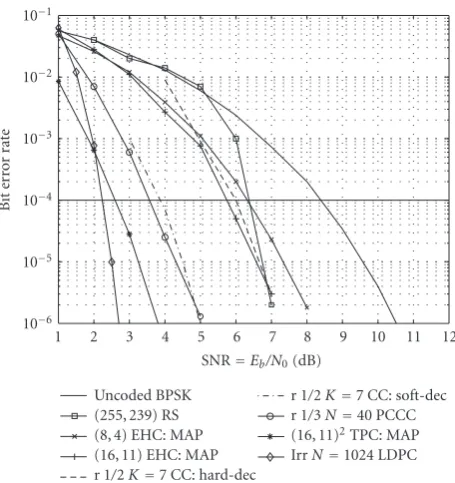
Figure 1 shows BER performance versus SNR for sev-eral types of error-correcting codes, compared to uncoded BPSK (binary phase-shift keying) modulation. Transmission is over an additive white Gaussian noise (AWGN) channel, with varianceN0/2 and zero mean, using BPSK modulation
10−1
10−2
10−3
10−4
10−5
10−6
Bi
t
er
ror
ra
te
1 2 3 4 5 6 7 8 9 10 11 12
SNR=Eb/N0(dB) Uncoded BPSK
(255, 239) RS (8, 4) EHC: MAP (16, 11) EHC: MAP r 1/2K=7 CC: hard-dec
r 1/2K=7 CC: soft-dec r 1/3N=40 PCCC (16, 11)2TPC: MAP IrrN=1024 LDPC
Figure1: BER performance versus SNR for several error-correcting codes.
for all encoded bits. Note that the SNR=Eb/N0in dB is an
energy ratio, rather than the power ratioS/N. The received energy per bitEb is energy per symbol over code rateEs/R, with constantEs, andN0is the noise power spectral density.
The thick black line indicates a BER of 10−4; the coding gain
for each code at this BER is easy to determine.
Three block codes are shown: a (255, 239, 17) Reed-Solomon code, an (8, 4, 4) extended Hamming code, and a (16, 11, 4) extended Hamming code. Note that the longer ex-tended Hamming code provides better performance due to its longer length. The Reed-Solomon code does not provide better performance until a much lower BER, even though it is significantly longer and has a better minimum distance, due to its higher rate.
Two convolutional codes, both rate 1/2 64-state con-straint length 7, are compared [45]. One uses a hard-decision Viterbi decoder and the other uses a soft-decision Viterbi de-coder. The soft-decision decoder performs about 2 dB better than the hard-decision decoder.
Three iteratively decoded codes are displayed as well, and the power of iterative decoding is clearly shown. These three codes provide the best performance on the graph. The paral-lel concatenated convolutional code (PCCC) is a classic turbo code, and used in the 3 GPP standard, although it is short; it has an interleaver and information sequence size of 40 bits, with a codeword length of 132 bits [46]. The (16, 11)2turbo
product code is composed of component (16,11) extended Hamming codes, decoded with MAP decoding [47]. The rate 1/2 length 1024 irregular LDPC is similar to the code imple-mented in [48], with 64 decoding iterations used.
Whether this coding gain ECCgain =SNRU −SNRECC
pro-vides sufficient energy savings due to the lowered minimum transmitted power requirement to outweigh the cost of extra power consumption due to the decoder will be examined in the next section.
4. ENERGY SAVINGS FROM ECC
4.1. Minimum required transmit power
For an uncoded system, the minimum required transmit powerPTX,U at the signal-to-noise ratio (termed SNRU) re-quired to achieve a desired BER is found from (4) and (7) to
whereηU is the uncoded system’s spectral efficiency. RNF is the receiver noise figure in dB and SNRUis the required SNR
=Eb/N0in dB to achieve the target BER with an uncoded
sys-tem. The path loss exponentndepends on the environment. At the frequencies of interest,d > λas stated inSection 2.2, so the far-field approximation of (8) is valid.
The uncoded system has a transmission rateRand band-widthB, so the uncoded spectral efficiencyηU = R/B. We consider BPSK-modulated transmission, which has a maxi-mum possible spectral efficiency ofηmax =1, and so we
re-quire thatB=RandηU =1.
For an equal comparison, we require that the coded sys-tem also have an information transmission rateR. Recall that the information bits are the uncoded bits before going into the encoder, and the coded bits are the bits output from the encoder. The number of coded bits is greater than the num-ber of information bits, so it would be an unfair comparison to consider the coded system to have a coded transmission rate ofR, as then the information transmission rate would decrease toR∗RC. The code rateRCis the number of infor-mation bits divided by the number of codeword bits. This means the uncoded system would be decodingR informa-tion bits per second, assuming BPSK modulainforma-tion, while the coded system would decode onlyR∗RCinformation bits per second. This would give the coded system an unfair advan-tage. Thus we require that the coded system transmit at an information transmission rate ofR, as for the uncoded sys-tem.
The coded transmission rate or coded channel through-putRthen increases toR=R/RC, for a code of rateRC. The bandwidth of the coded system,BC, is assumed to increase with the coded transmission rate, so thatBC =R. Thus the coded system’s spectral efficiency decreases toηC =R/BC =
RC.
Minimizing transmit power is considered herein to be the most critical parameter for a low-power WSN, whose battery lifetime is dependent on power consumption. There-fore all transmit power and energy calculations use the min-imum required transmit power and energy. In a low-power
WSN scenario, transmitting with as much power as possible, up to regulatory limits, is not desirable. Rather, transmitting with as little power as possible, so as to extend sensor bat-tery life, while maintaining a minimum required SNR, is our goal. Similar to a deep-space satellite scenario, the low-power WSN is far more low-power-constrained than bandwidth-constrained. In order to achieve power efficiency, we are will-ing to sacrifice spectral efficiency.
An equation similar to (10), but for the minimum re-quired transmit powerPTX,ECCusing ECC, can be found.
Re-call that the required SNRECCis less than SNRU by the cod-ing gain ECCgain. Also note that ηCBC = RandηUB = R. The minimum required transmit power when using ECC, PTX,ECC, is given by
The required transmit powerPTXis converted to required
transmit energy per transmitted information bit by dividing PTXby the information transmission rateRin bps to obtain
EbTX = PTX/Rin J/bit. Since the information transmission
rateRis the same for both uncoded and coded systems, the ratio of uncoded to coded energy per transmitted bit remains the same as for power. The information rateRis also assumed constant over all transmission distancesd. This allows for a straightforward comparison of the minimum required trans-mit energy and power of coded and uncoded systems at dif-ferent distances.
The transmit energy savings per information bit of the coded system is found as the difference between the mini-mum required transmit energy per information bit for un-coded and un-coded systems, as
EbTX,U[J/bit]=PTX,U
Use of ECC lowers the required minimum transmit power and energy per decoded bit as a result of the coding gain ECCgain. However, at the receiver, the coded system has
the added power consumption of its decoder, which must be factored in as a cost of using ECC. We do not consider the additional power consumed by the encoder; typically the en-coder is much smaller and consumes significantly less power than the decoder.
information throughput equal to the information transmis-sion rate R, and dividing the power consumption by the throughputRto get energy per decoded bitEbdec. However,
the power consumption values available for the implemen-tations are almost always for high throughput. A model is needed to estimate the decoder power consumed at through-put below that measured, based on the available power con-sumption data.
4.2. Decoder power consumption
The power consumption of a digital CMOS decoder consists of two types: dynamic and static. Dynamic power consump-tion is primarily due, in CMOS logic, to the switching capac-itance, and is modeled asPd ≈CVdd2 f, whereCis the total
switched capacitance,Vddis the power supply voltage, and f
is the operating, or clock, frequency. The static power con-sumption is due to leakage current and DC biasing sources, and can be modeled asPs=IleakVdd, whereIleakis the leakage
current. The total power consumption is modeled as [49]
Ptotal=Pd+Ps≈CVdd2 f +IleakVdd. (13)
The dynamic power consumption increases linearly with frequency, and becomes the dominant factor at higher fre-quencies. At low frequencies, static power consumption dominates and the total power consumption no longer in-creases linearly with frequency, but approaches the static value. This is seen from the total power consumption model as
Ptotal(f)≈a f+b, a=CVdd2,b=IleakVdd. (14)
The decoder throughputRis proportional tof over most of the range of f, so the total powerPtotal∝aR+b. At high
frequencies, near the limit of the clocking frequency, the dy-namic power will increase superlinearly with f, and the chip dissipates large amounts of power. We will not consider op-eration near the high-frequency limits of chip performance.
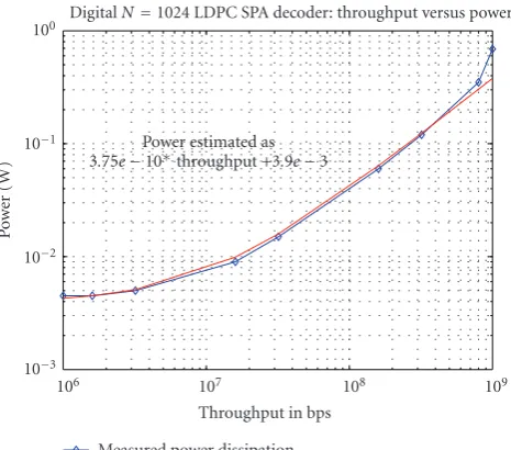
Figure 2shows actual power versus throughput measure-ments for a digital implementation of a length 1024 rate 1/2 LDPC decoder incorporating the sum-product algorithm (SPA) [48]. A linear approximation for the normalized power is compared to the actual measurement data. The linear ap-proximation is quite accurate in the linear, dynamic-power-dominated region of the power versus throughput curve.
From the decoder power consumption approximation, the energy cost per decoded information bit could be found asEbdec=Ptotal/R.
There is an additional factor to consider in power con-sumption, which is the implementation process. The decoder implementations presented inTable 1span several different CMOS processes: from 0.5μm to 0.16μm. Larger processes have higher supply voltage and dissipate greater amounts of power. So as not to unfairly penalize decoders implemented
100
10−1
10−2
10−3
Po
w
er
(W
)
106 107 108 109
Throughput in bps Measured power dissipation Approximated power dissipation
Power estimated as 3.75e−10∗throughput +3.9e−3
DigitalN=1024 LDPC SPA decoder: throughput versus power
Figure2: Power versus throughput: measured values and linear ap-proximation for digital LDPC implementation.
in a larger process size, we scale the energy per decoded bit byV2
dd. This results in an energy per decoded information bit
Ebdec, normalized to a supply voltage of 1 V, as
Ebdec= Ptotal
RV2
dd
. (15)
When operating anywhere in the dynamic power/high throughput region, the energy per decoded information bit is constant at
Ebdec= Pmax
RmaxVdd2
. (16)
This paper also considers analog decoder implementa-tions, which use very small bias currents, so that the tran-sistors operate in the subthreshold region. Hence, analog decoders inherently have very low power dissipation, and would seem a good choice for power-limited applications such as wireless sensor networks.
4.3. Energy savings of ECC and critical distance
Table1: Different decoder implementations: coding gain, maximum measured core power consumption and information throughput, and energy per decoded information bit, normalized toVdd=1, at maximum measured power and throughput.
Decoder implementation Coding gain in dB Pmaxin mW Rmaxin Mbps Vddin V Ebdecin nJ/bit Process size inμm
(255,239) RS digital 2 58 160 1.8 0.1193 0.18
Digital rate 1/2 CC hard-dec Viterbi 2.3 85 106 1.8 0.2475 0.18
Digital rate 1/2 CC soft-dec Viterbi 4.2 83 67 2.2 0.1138 0.35
(8,4) EHC analog 2 0.15 3.7 0.8 0.0633 0.18
(16,11) EHC analog 2.6 2.7 135 1.8 0.0062 0.18
(16, 11)2TPC analog 5.7 86.1 1000 1.8 0.0266 0.18
Rate 1/3 turbo analog 4.8 4.1 2 2 0.5125 0.35
N=1024 LDPC digital 6.1 630 500 1.5 0.56 0.16
(32,8,10) LDPC analog 1.3 5 80 1.8 0.0193 0.18
B=R. The energy savingsΔESis given by cal distancedCR. This is the distance at which use of a
par-ticular decoder implementation becomes energy-efficient. For sensors greater than a distance dCR apart, use of that
decoder implementation saves energy compared to an un-coded system. The critical distancedCR is found from (17)
as
Ptotalis represented as a linear function of the
through-putR, asPtotal=Pmax∗R/Rmax. Recall thatPmaxandRmaxare
the maximum measured power and throughput values, re-spectively, and they fall within the decoder’s dynamic power consumption region. The static power contribution is con-sidered to be negligible in the dynamic region. The factor of (1/R)1/nin (18) will be canceled, in the dynamic region, by RinPtotal. ThusdCRin the dynamic region is independent of
throughput, and has constant value. The critical distance is
given by
For a low throughput channel, we need to consider the type of network traffic across the channel. Bursty traf-fic, where long periods of silence are interspersed with brief bursts of data, is representative of many types of low throughput networks. Examples are weather sensors or pa-tient temperature sensors reporting conditions at fixed inter-vals, or sensors receiving data from security cameras at an isolated facility that only transmit data when there is move-ment or pixel change. Bursty traffic channels, while on av-erage low throughput, are better represented as a channel which has high throughput for a certain percentage of time, and no throughput the rest of the time.
In the bursty traffic scenario, a low throughput channel of rateRis viewed as having high throughput or transmission
rateR1> Rfor 100h% of the time, where 0≤h≤1, and no
throughput 100(1−h)% of the time, such thathR1=R. The
decoder is assumed to be powered down during periods of no throughput. During the time when the decoder is operating, throughput is high and decoder power consumption follows the dynamic power consumption model. Averaged over time, the total decoder power consumption is found to be
Ptotal=hR1Pmax
Rmax =
RPmax
Rmax
, (20)
the same as for the dynamic power consumption case. In other words, bursty traffic effectively lowers the dynamic power region to lower throughputs, because the data itself is delivered at a transmission rate within the dynamic power region.
Thus the critical distancedCR for low throughput with
Another factor to consider is whether the minimum re-quired uncoded transmit power, PTX,U, exceeds regulatory limits on maximum allowable transmitted power at a certain distancedPlim≤dCR. If so, then coding will be necessary
sim-ply to reduce the transmit power below regulatory limits. The critical distancedCR for the coded system would then drop
todPlim, provided that the minimum coded transmit power
PTX,ECCdid not also exceed the maximum power limitation.
There are many different regulatory limits, depending on location, frequency, and application. Thus it is not within the scope of this paper to determine whether PTX,U exceeds all possible limits at each frequency, application, and critical dis-tance. However, this is a factor which should be considered for actual usage.
The next section considers both digital and analog de-coder implementations and determines their critical dis-tances at various frequencies and environments. Path loss exponents range from n = 2 for free space to n = 4 for office space with many obstacles and ranging over multiple floors. Both high and bursty traffic low throughput channels are considered.
5. CRITICAL DISTANCE RESULTS FOR IMPLEMENTED DECODERS
5.1. Decoder implementations
We now examine several different decoder implementations, both analog and digital, for a variety of code types. BPSK transmission over an AWGN channel is assumed for all de-coders. Block codes considered include a high-rate digital (255, 239) Reed-Solomon decoder [50], an analog (8, 4, 4) extended Hamming decoder [51] and an analog (16, 11, 4) extended Hamming decoder [47]. Two digital convolutional decoders are included, a hard-decision Viterbi [52] and a soft-decision Viterbi decoder [53]. Both decoders use a rate 1/2, 64-state, constraint lengthK=7 convolutional code. It-erative decoders are examined as well. An analog rate 1/3 length 132 turbo decoder with interleaver size 40 [46] is con-sidered, as well as an analog (16, 11)2turbo product decoder
[47,54] using MAP decoding on each component (16, 11) extended Hamming codes. Two LDPC decoders are evalu-ated, a digital rate 1/2 length 1024 irregular LDPC sum-product decoder [48] and an analog rate 1/4 (32,8,10) regular LDPC min-sum decoder [55].
Table 1displays the pertinent data for each decoder, in-cluding coding gain in dB, maximum measured decoder core power consumption Pmax, corresponding maximum
mea-sured information (not coded) throughputRmax, core
sup-ply voltage Vdd. The decoded energy per information bit,
Ebdec, is found with (15), and assumes operation in either
the dynamic power consumption region or a bursty traffic low throughput scenario, which is modeled equivalently to the dynamic region. The coding gain is compared to uncoded BPSK at a BER of 10−4, and is the coding gain of the
imple-mented decoder. The process size for each decoder is also pre-sented. As shown, the analog decoders have the lowestEbdec
values.
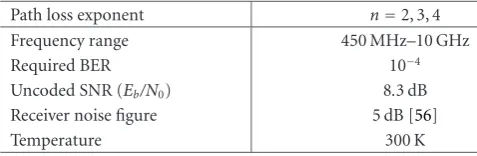
Table2: Parameters used in critical distance calculations.
Path loss exponent n=2, 3, 4
Frequency range 450 MHz–10 GHz
Required BER 10−4
Uncoded SNR (Eb/N0) 8.3 dB
Receiver noise figure 5 dB [56]
Temperature 300 K
5.2. Critical distance values
From the energy per decoded data bit,Ebdec, the critical
dis-tancedCR for each decoder implementation may be found
according to (19) for a variety of scenarios.
If we consider either a high throughput channel or a bursty traffic low throughput channel, thendCR, found from
(19), is independent of the throughput, with a single value regardless of throughput.
First we consider the path loss exponentn, as represen-tative of the transmission environment. We examinedCRfor
n=2, as a free space, line-of-sight (LOS) model, either out-doors or in a hallway; n = 3 as an interior environment such as an office building, where the network is all located on the same floor, or an outdoor environment such as for-est or foliated urban/suburban locations; andn = 4 as an interior environment with many obstructions and possibly multiple floors, or a dense urban environment. A frequency range from 450 MHz to 10 GHz is considered. Throughput is assumed to be either within the dynamic power region or low but bursty, and the critical distancedCRis calculated
ac-cording to (19). The parameters used in (19) are displayed in
Table 2.
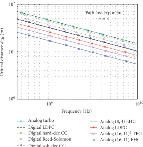
Figure 3showsdCRversus frequency forn=2, free space
path loss, for all decoders inTable 1. The decoder curves are shown in the order in which they appear in the graph legend, that is, top first.
At 10 GHz, the lowest critical distances belong to the ana-log (16,11) extended Hamming and (16, 11)2turbo product
decoders, at 30 and 48 m, respectively. These decoders would be practical in an indoor hallway scenario, where sensors placed at ends of the hallway would have LOS.
At lower frequencies, the values of dCR in a free space
environment, assuming no interference or extra background noise, are extremely large. Not untilf =3 GHz do any of the critical distances drop below 100 m. For an outdoor scenario where sensors are very widely spaced, with an LOS compo-nent, perhaps for either infrequently located security sensors around a large perimeter, along a highway or railroad track, monitoring outdoor weather data, or monitoring a fault line, the large distances even at lower frequencies might be practi-cal. The distances are far too large for any indoor scenario.
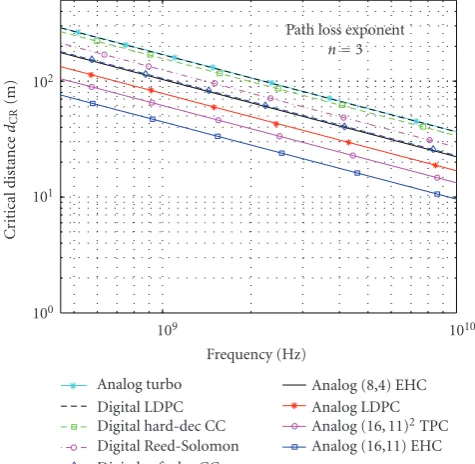
Figure 4showsdCRversus frequency forn=3, an office
environment or foliated outdoor environment.
104
103
102
101
100
C
ritical
distanc
e
dCR
(m)
109 1010
Frequency (Hz) Analog turbo
Digital LDPC Digital hard-dec CC Digital Reed-Solomon Digital soft-dec CC
Analog (8,4) EHC Analog LDPC Analog (16, 11)2TPC Analog (16,11) EHC Path loss exponent
n=2
Figure3: Estimated critical distancedCR versus f forn =2 free space path loss and high throughput or bursty low throughput channel.
(16, 11)2turbo product decoders again have the lowest
criti-cal distances, at 15 m and 21 m, respectively, for f =5 GHz, and 10 and 13 m at 10 GHz.
At the lowest frequency of 450 MHz, the lowest critical distance is 76 m for the (16,11) extended Hamming decoder, but all other decoders have critical distances above 100 m. Urban and suburban nodes which are not LOS, such as low buildings located more than a block apart, could be separated by distances greater than the critical distances even at the lowest frequencies, and well above the 2.4 GHz values. Out-door sensor networks in forested regions monitoring nest-ing sites, or forest health and dryness, or avalanche-prone regions, could also be spaced further apart than the critical distances at low frequencies.
Figure 5shows dCR versus frequency for n = 4, either
an office floor with many obstructions or between multiple floors, or a dense outdoor urban environment.
Critical distances, even at the lowest frequencies, are practical for a dense outdoor urban environment without LOS, for all decoders, as long as the sensors are spaced a few buildings apart.
For the office environment, the critical distance values are more practical for frequencies of 2 GHz and above. The analog decoders, with the exception of the analog turbo de-coder, all have critical distances below 25 m at 2 GHz, and 10 m or less at 10 GHz. The analog (16,11) extended Ham-ming and (16, 11)2 turbo product decoders again perform
the best, with respectivedCR values at 10 GHz of 5.5 m and
7 m, at 5 GHz of 8 and 10 m, and at 2.4 GHz of 12 and 15.5 m. These distances could represent a sensor network monitor-ing different floors of a building, with a node in each office,
102
101
100
C
ritical
distanc
e
dCR
(m)
109 1010
Frequency (Hz) Analog turbo
Digital LDPC Digital hard-dec CC Digital Reed-Solomon Digital soft-dec CC
Analog (8,4) EHC Analog LDPC Analog (16, 11)2TPC Analog (16,11) EHC Path loss exponent
n=3
Figure4: Estimated critical distancedCR versus f forn=3 path loss exponent and high throughput or bursty low throughput chan-nel.
or a network monitoring separate enclosures in an animal park.
These distances are just feasible, at the higher frequen-cies, to consider a sensor network for monitoring patients in a hospital. However, with additional interference and back-ground noise, as would be likely in these environments,dCR
would certainly decrease, increasing the energy efficiency of each decoder implementation and making ECC more practi-cal for this scenario.
The analog decoders, with their extremely low power consumption, provide the most energy-efficient decoding solution in these scenarios, except for the analog turbo de-coder. The digital decoders all have higherdCRvalues, from 2
to 4 times greater than the other analog decoders. For some scenarios, particularly free space transmission at frequencies below 1 GHz, ECC is not energy-efficient, except at very large distances. ECC is not always the best solution to minimizing energy. Our results fordCRclearly show that energy-efficient
use of ECC must consider the transmission environment and frequency, as well as decoder implementation. As the envi-ronment becomes more crowded, with more obstacles be-tween sensor nodes, ECC becomes more energy-efficient at shorter distances. At the highest frequencies, ECC is practi-cal for all the discussed scenarios when implemented with analog decoders.
5.3. Correction for power amplifier efficiency
Calculations presented so far have assumed that the power savings in RF transmitted powerPTXdirectly translate into
102
Figure5: Estimated critical distancedCR versus f forn=4 path loss exponent and high throughput or bursty low throughput chan-nel.
this assumption rarely holds true; in fact, both power factors are related through the power amplifier efficiencyε, defined as
ε= PTX
PDC.
(21)
Taking this into account, it is straightforward to show that (19), for high throughput or bursty traffic low through-put, needs to be modified as
dCR
In order to use the above equation, power efficiency numbers for typical CMOS implementations need to be eval-uated. As we will show below, εvaries from 19% to 65%, depending on what class power amplifier is used. The rea-sons for this wide spread of achieved efficiencies can be ex-plained as follows. Contemporary standards such as 802.11 use digital modulation to achieve high spectral efficiency. For example, at 54 Mbps, WLAN uses 64-QAM modulation on each OFDM subcarrier [57], resulting in a transmit wave-form with high peak-to-average ratio (PAR). A linear power amplifier must be used, which often has low power added ef-ficiency (PAE), resulting in high power consumption.
One step towards more power efficient drivers is to use constant envelope modulation, as in the personal area net-work standard 802.15.4.Constant envelope transmitters can be driven closer to the compression point, resulting in a
higher PAE; this in turn means lower power consumption. In this case, nonlinear (or switched-mode) power amplifiers may also be used, usually providing much higher efficiencies as a tradeofffor linearity. Typically, switched-mode ampli-fiers are also simpler in terms of realization complexity, war-ranting a more effective use of silicon area.
The highest efficiency of power amplification in silicon can be achieved using switched mode circuits [12]. Although theoretically, switched-mode PAs can transmit finite power with 100% efficiency, finite CMOS switching times and other effects result in lower efficiencies. As an example, a class E PA proposed in [58] has a PAE of 92.5% at an output power of
−4.3 dBm in the 433 MHz ISM band using duty-cycle mod-ulation (DCM). This efficiency figure, however, does not in-clude the power consumption of the DCM circuit (which is effectively a preamplifier circuit). Taking this into account reduces the overall PAE to 65%, providing a better parison towards other implementations. A somewhat com-parable linear amplifier shown in [3] has a drain efficiency of 27.5% at an output power of−4.2 dBm at f = 1.9 GHz (however, a given drain efficiency will always be higher than the equivalent PAE).
Efficiency values for several types of power amplifiers are presented inTable 3. Their efficiencyεvaries from 0.19, or 19%, to 0.65, with many common amplifier types showing εnear 0.3. At lower power output, as would be typical in a wireless sensor network,εmay drop even lower.
From (22),dCRwill change byε1/n, so assuming a power
efficiency of 33% and free space path loss,dCR will be 0.58
times the value obtained assuming ideal power efficiency of 100%. Forn=3,dCRis 0.69 times the ideal power efficiency
value ofdCR, and forn=4,dCRis 0.76 times the ideal power
efficiency value. If we assume even lower power efficiency of 19%,dCR reduces further to 0.44, 0.57, and 0.66 times its
value calculated assuming ideal power efficiency, forn =2, 3, and 4, respectively.
While these values do not dropdCRdramatically, they do
bring the n = 4 values at 10 GHz into the range of 3.5 to 7 m, and at 450 MHz to a range of 17 to 32 m, for the 4 most energy-efficient analog decoders with a power efficiency of 19%.
Figure 6shows the changes indCRobtained assumingε=
0.33 and 0.19, compared with ideal power efficiency ofε =
1, for the most energy-efficient decoder, the analog (16,11) extended Hamming decoder.
At f =10 GHz, a power efficiency of 33% dropsdCRin
free space from 30 m to 17 m, and 19% efficiency drops it fur-ther to 13 m. This is easily within the distance of one building to another, or from a house to a garage, for an LOS security scenario. Withn=3 and a power efficiency of 33%,dCRfalls
from 9.5 m to 6.5 m, and to 5.5 m with a power efficiency of 19%. For n = 4 and power efficiency of 33%,dCR is
Table3: Comparison of various power amplifier configurations.
Description Output power Efficiency Carrier frequency Notes Paper reference
Push-pull
linear −6.0 dBm 19% 900 MHz
Efficiency figure
includes oscillator [12] and frequency divider
Class B 9.8 dBm 38% 433 MHz Includes 3 class A
preamplifier stages [14]
Class A/B 2.7 dBm 33% 1.9 GHz N/A [59]
Class E −4.3 dBm 65% 433 MHz Uses duty-cycle
modulation [58]
OOK
−4.2 dBm 27.5% 1.9 GHz N/A
cascode [3]
104
103
102
101
100
C
ritical
distanc
e
dCR
(m)
109 1010
Frequency (Hz) n=2, Eff=100%
n=2, Eff=33% n=2, Eff=19% n=3, Eff=100% n=3, Eff=33%
n=3, Eff=19% n=4, Eff=100% n=4, Eff=33% n=4, Eff=19% Analog (16,11) EHC
n=2
n=3 n=4
Figure 6: Estimated critical distance dCR for analog (16,11) ex-tended Hamming decoder assuming 19%, 33%, and 100% power efficiency, forn=2, 3, and 4.
6. CONCLUSIONS
In free space line-of-sight scenarios, ECC is not very energy-efficient for frequencies below 2 GHz, except for widely spaced outdoor monitoring networks. In an urban out-door setting, at higher frequencies, ECC can be practical for sensor networks placed between buildings, especially when implemented with analog decoders. For indoor environ-ments, ECC is energy-efficient at high frequencies, for sen-sors placed at opposite ends of hallways or in adjacent rooms, or on multiple floors or in a dense urban environment at all frequencies. Analog decoders offer the most energy-efficient ECC solution, becoming energy-efficient at distances from 1/4 to 1/2 the critical distances of the digital decoders exam-ined in this paper.
The effect of interference from other radiating sources has not been taken into account in this paper. This would re-ducedCRvalues, as the uncoded system must increase power
to overcome the interference. The ECC system will thus be-come more energy-efficient at shorter distances when inter-ference is considered.
The analog decoders in general, with their low power consumption, are better suited than digital decoders for the low-power requirements of wireless sensor networks. How-ever, even the analog decoders require distances of 5–10 m (3.5–7 m for 19% power amplifier efficiency) at 10 GHz and n=4 before they are energy-efficient in terms of the power the decoder consumes compared with the energy saved due to coding gain. Thus, analog decoders may not yet be practi-cal for sensor network applications requiring close spacing of the sensors, such as monitoring patients in a crowded emer-gency room, babies in a nursery, or multiple sensors on one patient. Again, the effect of interference has not been consid-ered, and in these scenarios where sensors are spaced closely together, interference could well be sufficient to require ECC for reliable operation.
The analog decoder critical distances considered for 10 GHz andn=4 without interference are practical for sen-sors at ends of a room, or located one per room, such as air quality and temperature/humidity sensors, or sensors mitting experimental data between university labs, or trans-mitting patient data during a procedure to equipment in an-other room.
ACKNOWLEDGMENTS
Many thanks to Vincent Gaudet and Chris Winstead, for their helpful comments and suggestions regarding analog de-coders and throughput, and to the editor and reviewers for their recommendations to improve the quality of this paper.
REFERENCES
[1] S. Roundy, B. Otis, Y. H. Chee, J. Rabaey, and P. Wright, “A 1.9GHz RF transmit beacon using environmentally scavenged energy,” inProceedings of IEEE International Symposium on Low Power Electronics and Devices (ISLPED ’03), Seoul, Korea, August 2003.
[2] T.-H. Lin, W. J. Kaiser, and G. J. Pottie, “Integrated low-power communication system design for wireless sensor networks,”
IEEE Communications Magazine, vol. 42, no. 12, pp. 142–150, 2004.
[3] B. Otis, Y. H. Chee, and J. Rabaey, “A 400μW-RX, 1.6mW-TX super-regenerative transceiver for wireless sensor networks,” inProceedings of IEEE International Solid-State Circuits Con-ference (ISSCC ’05), vol. 1, pp. 396–397, San Francisco, Calif, USA, February 2005.
[4] K. Iniewski, C. Siu, S. Kilambi, et al., “Ultra-low-power circuit and system design tradeoffs for smart sensor network appli-cations,” inProceedings of the International Conference on In-formation and Communication Technology (ICICT ’05), Cairo, Egypt, December 2005, invited paper.
[5] V. Ekanayake, C. Kelly IV, and R. Manohar, “An ultra-low-power processor for sensor networks,” in Proceedings of the 11th International Conference on Architectural Support for Pro-gramming Languages and Operating Systems (ASPLOS-XI ’04), Boston, Mass, USA, October 2004.
[6] G. K. Ottman, H. F. Hofmann, and G. A. Lesieutre, “Opti-mized piezoelectric energy harvesting circuit using step-down converter in discontinuous conduction mode,”IEEE Transac-tions on Power Electronics, vol. 18, no. 2, pp. 696–703, 2003. [7] S. Roundy, D. Steingart, L. Fr´echette, P. K. Wright, and J.
Rabaey, “Power sources for wireless sensor networks,” in Pro-ceedings of the 1st European Workshop on Wireless Sensor Net-works (EWSN ’04), pp. 1–17, Berlin, Germany, January 2004. [8] W. Ye, J. Heidemann, and D. Estrin, “An energy-efficient MAC
protocol for wireless sensor networks,” inProceedings of 21st International Conference of IEEE Computer and Communica-tions Societies (INFOCOM ’02), vol. 3, pp. 1567–1576, New York, NY, USA, June 2002.
[9] K. Sohrabi and G. J. Pottie, “Performance of a novel self-organization protocol for wireless ad-hoc sensor networks,” inProceedings of IEEE 50th Vehicular Technology Conference (VTC ’99), vol. 2, pp. 1222–1226, Amsterdam, The Nether-lands, September 1999.
[10] A. Woo and D. Culler, “A transmission control scheme for me-dia access in sensor networks,” inProceedings of ACM/IEEE In-ternational Conference on Mobile Computing and Networking (MOBICOM ’01), Rome, Italy, July 2001.
[11] F. Bennett, D. Clarke, J. B. Evans, A. Hopper, A. Jones, and D. Leask, “Piconet: embedded mobile networking,”IEEE Personal Communications, vol. 4, no. 5, pp. 8–15, 1997.
[12] A. Molnar, B. Lu, S. Lanzisera, B. W. Cook, and K. S. J. Pis-ter, “An ultra-low power 900 MHz RF transceiver for wireless sensor networks,” inProceedings of the IEEE on Custom Inte-grated Circuits Conference (CICC ’04), pp. 401–404, Orlando, Fla, USA, October 2004.
[13] A.-S. Porret, T. Melly, D. Python, C. C. Enz, and E. A. Vittoz, “An ultralow-power UHF transceiver integrated in a standard digital CMOS process: architecture and receiver,”IEEE Journal of Solid-State Circuits, vol. 36, no. 3, pp. 452–466, 2001. [14] T. Melly, A.-S. Porret, C. C. Enz, and E. A. Vittoz, “An
ultralow-power UHF transceiver integrated in a standard dig-ital CMOS process: transmitter,”IEEE Journal of Solid-State Circuits, vol. 36, no. 3, pp. 467–472, 2001.
[15] P. Lettieri, C. Fragouli, and M. B. Srivastava, “Low power er-ror control for wireless links,” inProceedings of the 3rd Annual ACM/IEEE International Conference on Mobile Computing and Networking (MOBICOM ’97), pp. 139–150, Budapest, Hun-gary, September 1997.
[16] S. Mukhopadhyay, D. Panigrahi, and S. Dey, “Data aware, low cost error correction for wireless sensor networks,” in Proceed-ings of IEEE Wireless Communications and Networking Confer-ence (WCNC ’04), vol. 4, pp. 2492–2497, Atlanta, Ga, USA, March 2004.
[17] E. Shih, S. Cho, F. S. Lee, B. H. Calhoun, and A. Chandrakasan, “Design considerations for energy-efficient radios in wireless microsensor networks,”Journal of VLSI Signal Processing Sys-tems for Signal, Image, and Video Technology, vol. 37, no. 1, pp. 77–94, 2004.
[18] C. Berrou, A. Glavieux, and P. Thitimajshima, “Near Shannon limit error-correcting coding and decoding: turbo-codes,” in
Proceedings of IEEE International Conference on Communica-tions (ICC ’93), vol. 2, pp. 1064–1070, Geneva, Switzerland, May 1993.
[19] R. G. Gallager, “Low-density parity-check codes,”IRE Trans-actions on Information Theory, vol. 8, no. 1, pp. 21–28, 1962. [20] S. Kasnavi, S. Kilambi, B. Crowley, K. Iniewski, and B.
Kamin-ska, “Application of error control codes (ECC) in ultra-low-power RF transceivers,” inProceedings of IEEE Dallas Circuits and Systems Workshop (DCAS ’05), Dallas, Tex, USA, Septem-ber 2005.
[21] N. Sadeghi, S. L. Howard, S. Kasnavi, K. Iniewski, V. C. Gaudet, and C. Schlegel, “Analysis of error control code use in ultra-low-power wireless sensor networks,” inProceedings of IEEE International Symposium on Circuits and Systems (IS-CAS ’06), Kos, Greece, May 2006, accepted.
[22] C. Schlegel and L. Perez,Trellis and Turbo Coding, IEEE/Wiley, Piscataway, NJ, USA, 2004.
[23] B. Sklar,Digital Communications: Fundamentals and Applica-tions, Prentice Hall, Englewood Cliffs, NJ, USA, 1988. [24] W. L. Stutzman and G. A. Thiele,Antenna Theory and Design,
John Wiley & Sons, New York, NY, USA, 2nd edition, 1998. [25] T. S. Rappaport,Wireless Communications: Principles and
Prac-tice, Prentice Hall, Englewood Cliffs, NJ, USA, 1996.
[26] S. Y. Seidel and T. S. Rappaport, “Path loss prediction in multi-floored buildings at 914 MHz,”IEE Electronics Letters, vol. 27, no. 15, pp. 1384–1387, 1991.
[27] C. Perez-Vega and J. L. Garcia, “A simple approach to a statis-tical path loss model for indoor communications,” in Proceed-ings of the 27th European Microwave Conference and Exhibition, pp. 617–623, Jerusalem, Israel, September 1997.
[28] G. D. Durgin, T. S. Rappaport, and H. Xu, “Partition-based path loss analysis for in-home and residential areas at 5.85 GHz,” inProceedings of IEEE Global Telecommunications Con-ference (GLOBECOM ’98), vol. 2, pp. 904–909, Sydney, NSW, Australia, November 1998.
Conference on Communications (ICC ’02), vol. 5, pp. 3424– 3428, New York, NY, USA, April-May 2002.
[30] J. Hansen and P. E. Leuthold, “The mean received power in ad hoc networks and its dependence on geometrical quantities,”
IEEE Transactions on Antennas and Propagation, vol. 51, no. 9, pp. 2413–2419, 2003.
[31] D. M. J. Devasirvatham, C. Banerjee, M. J. Krain, and D. A. Rappaport, “Multi-frequency radiowave propagation mea-surements in the portable radio environment,” in Procced-ings of IEEE International Conference on Communications (ICC ’90), vol. 4, pp. 1334–1340, Atlanta, Ga, USA, April 1990. [32] T. J. Harrold, A. R. Nix, and M. A. Beach, “Propagation
stud-ies for mobile-to-mobile communications,” inProceedings of IEEE 54th Vehicular Technology Conference (VTC ’01), vol. 3, pp. 1251–1255, Atlantic City, NJ, USA, October 2001. [33] H. Hashemi, “The indoor radio propagation channel,”
Pro-ceedings of the IEEE, vol. 81, no. 7, pp. 941–968, 1993. [34] J. Sydor, “True broadband for the countryside,”IEE
Commu-nications Engineer, vol. 2, no. 2, pp. 32–36, 2004.
[35] A. Aguiar and J. Gross, “Wireless channel models,” Tech. Rep. TKN-03-007, Telecommunications Networks Group, Technische Universit¨at Berlin, Berlin, Germany, April 2003. [36] R. W. Hamming, “Error detecting and error correcting codes,”
The Bell System Technical Journal, vol. 29, no. 2, pp. 147–160, 1950.
[37] I. S. Reed and G. Solomon, “Polynomial codes over certain finite fields,”SIAM Journal on Applied Mathematics, vol. 8, pp. 300–304, 1960.
[38] R. C. Bose and D. K. Ray-Chaudhuri, “On a class of error cor-recting binary group codes,”Information and Control, vol. 3, pp. 68–79, 1960.
[39] A. Hocquenghem, “Codes correcteurs d’erreurs,” Chiffres, vol. 2, pp. 147–156, 1959.
[40] A. J. Viterbi, “Error bounds for convolutional codes and an asymptotically optimum decoding algorithm,”IEEE Transac-tions on Information Theory, vol. 13, no. 2, pp. 260–269, 1967. [41] L. R. Bahl, J. Cocke, F. Jelinek, and J. Raviv, “Optimal decod-ing of linear codes for minimizdecod-ing symbol error rate,”IEEE Transactions on Information Theory, vol. 20, no. 2, pp. 284– 287, 1974.
[42] J. Pearl,Probabilistic Reasoning in Intelligent Systems: Networks of Plausible Inference, Morgan Kaufmann, San Mateo, Calif, USA, 1988.
[43] N. Wiberg, “Codes and decoding on general graphs,” thesis of Doctor of Philosophy, Link¨oping University, Link¨oping, Swe-den, 1996.
[44] M. P. C. Fossorier, M. Mihaljevi´c, and H. Imai, “Reduced com-plexity iterative decoding of low-density parity check codes based on belief propagation,”IEEE Transactions on Commu-nications, vol. 47, no. 5, pp. 673–680, 1999.
[45] J. G. Proakis, Digital Communications, McGraw-Hill, New York, NY, USA, 4th edition, 2001.
[46] D. Vogrig, A. Gerosa, A. Neviani, A. Graell I Amat, G. Mon-torsi, and S. Benedetto, “A 0.35-μm CMOS analog turbo de-coder for the 40-bit rate 1/3 UMTS channel code,”IEEE Jour-nal of Solid-State Circuits, vol. 40, no. 3, pp. 753–761, 2005. [47] C. Winstead, “Analog Iterative Error Control Decoders,”
the-sis of Doctor of Philosophy, Department of Electrical & Com-puter Engineering, University of Alberta, Alberta, Canada, 2004.
[48] A. J. Blanksby and C. J. Howland, “A 690-mW 1-Gb/s 1024-b, rate-1/2 low-density parity-check code decoder,”IEEE Journal of Solid-State Circuits, vol. 37, no. 3, pp. 404–412, 2002. [49] J. Rabaey, A. Chandrakasan, and B. Nikolic,Digital Integrated
Circuits, Prentice Hall, Englewood Cliffs, NJ, USA, 2nd edi-tion, 2003.
[50] T. S. Fill and P. G. Gulak, “An assessment of VLSI and embed-ded software implementations for Reed-Solomon decoders,” inProceedings of IEEE Workshop on Signal Processing Systems (SIPS ’02), pp. 99–102, San Diego, Calif, USA, October 2002. [51] C. Winstead, N. Nguyen, V. C. Gaudet, and C. Schlegel,
“Low-voltage CMOS circuits for analog iterative decoders,” IEEE Transactions on Circuits and Systems I: Regular Papers, vol. 52, no. 4, 2005.
[52] M. Kawokgy, C. Andre, and T. Salama, “Low-power asyn-chronous Viterbi decoder for wireless applications,” in Pro-ceedings of the International Symposium on Low Power Elec-tronics and Design (ISLPED ’04), pp. 286–289, Newport, Calif, USA, August 2004.
[53] C.-C. Lin, C.-C. Wu, and C.-Y. Lee, “A low power and high speed Viterbi decoder chip for WLAN applications,” in Pro-ceedings of the 29th European Solid-State Circuits Conference (ESSCIRC ’03), pp. 723–726, Lissabon, Portugal, September 2003.
[54] C. Winstead, C. Schlegel, and V. C. Gaudet, “CMOS analog de-coder for (256,121) block turbo code,” submitted toEURASIP Journal on Wireless Communications and Networking, special issue: CMOS RF circuits for wireless applications.
[55] S. Hemati, A. H. Banihashemi, and C. Plett, “An 80-Mb/s
0.18-μm CMOS analog min-sum iterative decoder for a (32,8,10) LDPC code,” inProceedings of the IEEE Custom Integrated Cir-cuits Conference (CICC ’05), pp. 243–246, San Jose, Calif, USA, September 2005.
[56] T. Lee,The Design of CMOS Radio-Frequency Integrated Cir-cuits, Cambridge University Press, Cambridge, UK, 2nd edi-tion, 2004.
[57] “Wireless LAN medium access control (MAC) and physical layer (PHY) specification,”LAN MAN Standards Committee, IEEE Computer Society, IEEE, New York, NY, USA, IEEE Std 802.11 - 1997 edition, 1997.
[58] D. Aksin, S. Gregori, and F. Maloberti, “High-efficiency power amplifier for wireless sensor networks,” inProceedings of the IEEE International Symposium on Circuits and Systems (IS-CAS ’05), vol. 6, pp. 5898–5901, Kobe, Japan, May 2005. [59] Y. H. Chee, J. Rabaey, and A. M. Niknejad, “A class A/B low
power amplifier for wireless sensor networks,” inProceedings of the IEEE International Symposium on Circuits and Systems (ISCAS ’04), vol. 4, pp. 409–412, Vancouver, BC, Canada, May 2004.
Christian Schlegel received the Dipl. El. Ing. ETH degree from the Federal Institute of Technology, Zurich, in 1984, and the M.S. and Ph.D. degrees in electrical engineering from the University of Notre Dame, Notre Dame, Ind, in 1986 and 1989. He held aca-demic positions at the University of South Australia, University of Texas, and Univer-sity of Utah, Salt Lake City. In 2001 he was named iCORE Professor for High-Capacity
Digital Communications at the University of Alberta, Canada, a 3-million-dollar research program in leading-edge digital commu-nications. His interests are in error control coding and applica-tions, multiple access communicaapplica-tions, digital communicaapplica-tions, and analog and digital implementations of communications sys-tems. He is the author ofTrellis CodingandTrellis and Turbo Cod-ingby IEEE/Wiley, andCoordinated Multiple User Communications, coauthored with Professor Alex Grant. He received a 1997 Career Award, and a Canada Research Chair in 2001. He is an Associate Editor for coding theory and techniques for IEEE Transactions on Communications, and a Guest Editor of the IEEE Proceedings on Turbo Coding. He served as Technical Program Cochair of ITW ’01 and ISIT ’05, and General Chair of CTW ’05, as well as on numer-ous technical conference program committees.
Kris Iniewskiis an Associate Professor at the Electrical and Computer Engineering Department of University of Alberta. He is also a President of CMOS Emerging Tech-nologies, Inc., a consulting company in Vancouver. His research interests are in ad-vanced CMOS devices and circuits for ultra-low-power wireless systems, medical imag-ing, and optical networks. From 1995 to 2003, he was with PMC-Sierra and held
var-ious technical and management positions in research & develop-ment and strategic marketing. Prior to joining PMC-Sierra, from 1990 to 1994, he was an Assistant Professor at the University of Toronto’s Electrical and Computer Engineering Department. He has published over 80 research papers in international journals and conferences. He holds 18 international patents granted in USA, Canada, France, Germany, and Japan. He is a frequent invited speaker and consults for multiple organizations internationally. He received his Ph.D. degree in electronics (with honors) from the Warsaw University of Technology (Warsaw, Poland) in 1988. To-gether with Carl McCrosky and Dan Minoli he is an author of
Data Networks-VLSI and Optical Fibre(Wiley, 2006) and editor of