Improving ambiguity resolution by applying ionosphere corrections
from a permanent GPS array
Dennis Odijk
Department of Mathematical Geodesy and Positioning, Delft University of Technology, Thijsseweg 11, 2629 JA Delft, The Netherlands
(Received January 6, 2000; Revised June 26, 2000; Accepted July 5, 2000)
Fast and high precision relative GPS positioning over distances up to 100 km is mainly limited by errors in the GPS signals due to propagation through the Earth’s ionosphere. With permanent GPS arrays, which are present in many countries nowadays, it becomes possible to correct a user’s GPS measurements to a certain extent for these ionospheric delays. A way to do so is to interpolate the ionospheric delays which have been estimated from the network of permanent stations. When these ‘interpolated corrections’ are applied to the user’s data, the ionospheric delays may be reduced, which may lead to an improved ambiguity resolution for his (long) baseline.
1.
Introduction
Integer GPS carrier phase ambiguity resolution is a pre-requisite to get very precise positioning results using short observation time spans. Ionospheric errors in the relative GPS observations over baselines of medium lengths (longer than 10 km) hamper a fast estimation of the integer carrier phase ambiguities. This problem is expected to grow in the coming maximum of the sunspot cycle (expected in the years 2000–2002). If a permanent GPS array is within the vicinity, then this can be an outcome, as it is possible to estimate pre-cise ionospheric delays from the network. These estimates can then be interpolated for an arbitrary location within the surroundings of the network and these interpolated values can be provided to users to correct their GPS measurements. In the Netherlands such an ionosphere interpolation technique will be part of the so-called Virtual GPS Reference Station concept (as explained in van der Marel, 1998). This means that the observation data of the Dutch permanent stations are transformed to a location, which is approximately the posi-tion of the user’s antenna, and these data are corrected for the errors that may be expected at the user’s location. Next, the user processes these virtual data together with the data of his receiver as an ordinary ‘short baseline’.
The purpose of this article is to gain insight in how well the ionospheric errors that are interpolated from the perma-nent stations coincide with the true ionospheric errors at the location of the virtual station. To test this performance, pro-visional tests have been carried out with samples of data of the Southern California Integrated GPS Network (SCIGN). The reason of not using data of the permanent network in the Netherlands, is that the SCIGN network is very dense and no additional measurements were necessary. Besides, the SCIGN data are very well archived and freely available athttp://www.scign.org. Furthermore, the
geomag-Copy right cThe Society of Geomagnetism and Earth, Planetary and Space Sciences (SGEPSS); The Seismological Society of Japan; The Volcanological Society of Japan; The Geodetic Society of Japan; The Japanese Society for Planetary Sciences.
netic latitude of the SCIGN network is close to that of the Dutch network (both are located in the geomagnetic mid-latitudes) and due to the geomagnetic latitude dependence of the ionospheric activity similar ionospheric errors may be expected (see Klobuchar, 1991).
2.
Fast Positioning in a Permanent GPS Array
The permanent GPS array in the Netherlands, which is called the AGRS.NL (Active GPS Reference System), con-sists of five stations, with separations of 100–200 km. As a consequence, for a user operating in the Netherlands, the distance to the nearest AGRS.NL reference station can be as large as 100 km. This means that in order to obtain a precise position, most of the times he has to account for significant ionospheric delay errors in his measurements.
To explain this, consider the general mathematical model to process (relative) GPS observations. The model of dual-frequency phase and code observation equations in double-difference (DD) mode reads for at least two receivers si-multaneously tracking at least four satellites at observation epochi:
φ1(i)=B(i)b+λ1a1−I(i) φ2(i)=B(i)b+λ2a2−(λ22/λ21)I(i) p1(i)=B(i)b+I(i)
p2(i)=B(i)b+(λ22/λ21)I(i)
(1)
In this model φ1 and φ2 are the
‘observed-minus-computed’ DD phase observables (in units of meters rather than cycles) on L1 and L2 respectively andp1andp2denote
the observed-minus-computed DD code (pseudo-range) ob-servables on L1 and L2. The vectorbrepresents the incre-ments of the components of the baseline coordinates, whereas the matrix B(i)contains the receiver-satellite unit vectors. The known wavelengths are denoted asλ1 andλ2, anda1
anda2are the unknown but time-invariant DD phase ambi-guities. Furthermore, I(i)is the DD form of the unknown
slant ionospheric delays on the L1-frequency. Note that in model (1) no unknowns for tropospheric, orbit, multipath as well as other errors have been introduced. These are sup-posed to be sufficiently small or accounted for by models or corrections.
Resolution of theintegerDD ambiguities makes precise positioning feasible using very short observation time spans. Therefore, to model (1) integer constraints are added, which are denoted asaj ∈Z,(j =1,2), withZbeing the space of
integer numbers. However, the inclusion of the ionospheric unknowns in model (1) hampers aquickresolving of the in-teger ambiguities. Only in case of moderate ionospheric cir-cumstances at the mid-latitude regions, for baselines shorter than about 10 km the relative ionospheric delays are so small that they may be neglected. For such short baselines it has already been extensively shown in the literature that the (cor-rect) integer ambiguities can be estimated in very short time spans, see e.g. Tiberiuset al.(1997). For precise positioning purposes within the AGRS.NL network however, usually a user has to account for the non-negligible ionospheric delays in his observations. If the ionospheric delays are estimated from the observations simultaneously with the other param-eters according to model (1), the minimum time to success-fully resolve the integer ambiguities is typically 30 minutes or more. For many applications this time span will be too long. A better idea is to reduce the ionospheric errors in the observations and not to estimate any parameters, which can be realized by correcting the user’s data withinterpolations
of the ionospheric delays estimated at the permanent stations.
3.
Interpolation of Network Ionospheric Delays
In this section it will be explained how the ionospheric interpolations at the site of a user can be generated from the GPS data at the permanent stations.
In afirst step, the observed data at the permanent stations are processed according to the model (1). Using a relatively long time span of data (i.e. about 1 hour with a sampling of 30 sec.) and the known positions of the permanent stations, the integer ambiguities can be resolved correctly. In a next step, with the integer ambiguities heldfixed, estimates for the ionospheric delays between these permanent stations are obtained. These so-called ambiguity-fixed estimates of the DD ionospheric delays (which have a very high precision if the correct ambiguities have been resolved) form the input of an interpolation algorithm, which is based on the spatial correlation between these relative ionospheric delays.
This interpolation for a certain user locationxwith respect to a pivot location (here: permanent station 1) is carried out for each individual observation epoch and each satellites
(with respect to a pivot satellite p). The interpolated DD ionospheric delay,I1xps, can be computed, according to (van der Marel, 1998), as: the DD ionospheric delays at thenpermanent stations andcs
kt
is a spatial covariance function. Note that in the interpolation algorithm (2) the DD ionospheric delay at the pivot station
ˆ
I11ps has been added while this, by definition, equals zero. The reason for doing this is to take the geometry at the pivot station into account. Furthermore, note when applying the algorithm (2) for the locations of the permanent stations, their ionospheric input values are obtained: I1rps= ˆI1rps(r =
1, . . . ,n).
Important to the performance of the interpolation is the choice of the spatial covariance function cskt. In the tests which will be described in Section 5 a spatial covariance function is assumed, which is a linearfunction of the dis-tances between theionospheric pierce pointsof the perma-nent stations: cs
kt = lmax −lskt, wherel s
kt is the geometric
distance between the ionospheric points of receivers kand
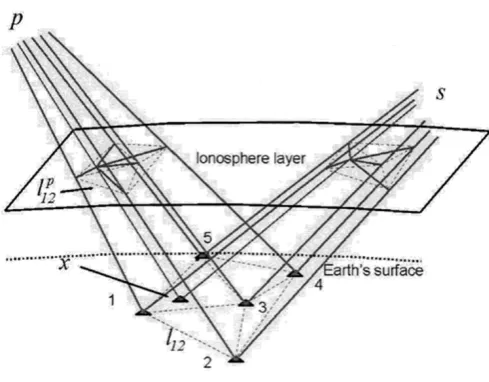
t and withlmax = ∞. Note that a ionospheric pierce point
is the intersection of the receiver-satellite line of sight with a single ionosphere layer (see Georgiadou and Kleusberg, 1988), which is here assumed sphere-like at a height of 350 km above the Earth, see Fig. 1. It is known that at a height of 350 km the GPS signals are mostly affected by the free electrons in the ionosphere and therefore the interpolation is performed at this‘ionosphere level’and not at ground level. The spatial covariance is chosen such that the covariance be-tween two points is decreasing when the distance bebe-tween these points is increased. This assumption is supposed to be valid as theabsoluteionospheric delays for receivers at relatively close distance (maximum 200 km) tend to be very similar. The setting oflmax = ∞in the spatial covariance
function has been done to make the interpolation results in-dependent of the choice of pivot station. Although an infi-nite value is not allowed considering the single covariance function, itis allowed when it is used in the interpolation algorithm (2).
Fig. 2. Used stations of the SCIGN network in the tests: LINJ-TRAK-WIDC-SIO3-SNI1 (black stars—the‘permanent’stations) and CIT1-CRFP-BILL-MONP (grey stars—the‘user’stations). Note that the dotted lines are dependent baselines and that the user baselines all are all formed with the closest permanent station as reference station.
4.
Ambiguity Resolution with the Ionospheric
Corrections Applied
The topic of this article is to study how well the interpo-lation is able to predict the‘real’DD ionospheric delays at a position within a permanent network, even in periods of increasing ionospheric activity. This performance will be measured in terms of shortening of the time to successfully fix the integer ambiguities when the interpolated corrections are applied.
For this purpose, data from the SCIGN network has been used. In Fig. 2 the configuration of the stations used in the tests is shown. The SCIGN stations which are assigned as ‘permanent’stations in the tests are 100–200 km separated from each other and the assigned‘user’stations all lie within 50–80 km from the nearest‘permanent’station. Note that station MONP lies outside of the network.
In afirst step of the tests, ionospheric delays between the ‘permanent’stations (pivot station LINJ) have been estimated for 1 hour of data collected at 30 sec. sampling interval ac-cording to model (1), with some modifications: no estimation of baseline coordinates (they are accurately known in case of a permanent network), and extension of the model with a tropospheric zenith delay parameter per station, because of considerable height differences between the permanent stations.
Next, the interpolated corrections at the user stations were computed using (2) and applied to the data of the user sta-tions and their closest permanent stasta-tions. To measure the improvement of ambiguity resolution, the following proce-dure has been used:
1. Estimate a reference set of integer ambiguities. A reference set of integer ambiguities (“ground-truth”) at each user baseline was obtained using model (1), thuswith
ionospheric parameters estimated. These ambiguities could be resolved as the full hour of observations was processed. (Of course, in real practice these reference ambiguities can-not be obtained as only data of short time spans are available, and one has to rely on other ambiguity validation techniques.)
2. Process short time spans with and without interpolated
corrections and compute ambiguity success rates.
Next, the 1-hour data sets at the user stations were divided into smaller windows to test whether the same integers as in step 1 could be resolvedwithoutthe estimation of ionospheric parameters, butwiththe data a priori corrected. The selected time windows are: 1 epoch (instantaneous ambiguity resolu-tion), 12 epochs (time span 5 min.) and 20 epochs (10 min.). The estimated integers in this step were compared with those of step 1 and asuccess ratewas obtained by taking the ratio of the number of correct ambiguity sets and the total number of ambiguity sets. To gain insight in the improvement for each baseline also integer success rates were estimated when the data were processed without estimation of ionospheric paremeters andwithoutany corrections applied.
In all tested cases, the assumed stochastic modelof the observations is rather simple: all observations were uncor-related assumed with a standard deviation of 3 mm for the (undifferenced) phase and 30 cm for the (undifferenced) code observations. For all processing theGPSveQsoftware of the Delft University of Technology (de Jonge, 1998) was used, which contains theLAMBDA-methodfor least-squares esti-mation of the integer ambiguities (see Teunissen, 1993).
5.
Test Results
The results of two tests will be described. Thefirst data set was collected in winter on 1 January 1999, during the time span 20:00:30–21:00:00 UTC (12:00:30–13:00:00 lo-cal time). This data set was selected because during this period ionospheric activity was disturbed due to the occur-rence of‘travelling ionospheric disturbances’(TIDs). These TIDs mainly occur during winter months around local noon and cause a sudden change in the size of the relative iono-spheric delays (see Wanninger, 1999). The second data set was collected in summer on 24 June 1999 and it is known that during this period the ionospheric activity was much less disturbed. Essentially, the same stations were used in both tests, the only difference being in the use of user station BILL rather than CRFP (see Fig. 2).
5.1 Test data set 1: 1 January 1999
In Fig. 3 time-series of the estimated DD ionospheric de-lays are given for the permanent stations. In this test 6 satel-lites have been used and the double-differences all hold with respect to PRN2. From the graphs one can see that the time-series are smooth butfluctuating which is probably caused by TIDs.
Fig. 3. Estimated DD ionospheric delays at permanent stations (from left to right: SNI1-TRAK-SIO3-WIDC) with respect to pivot station LINJ and pivot satellite PRN 2 on 1 January 1999, 20:00:30–21:00:00 UTC.
Table 1. Ambiguity resolution success rates with and without ionospheric corrections applied (1 January 1999).
Ambiguity Without interpolated corrections With interpolated corrections
Success-rate LINJ-CIT1 WIDC-CRFP SIO3-MONP LINJ-CIT1 WIDC-CRFP SIO3-MONP
(58 km) (66 km) (78 km) (58 km) (66 km) (78 km)
Instantaneous 7% 0% 0% 31% 44% 9%
5 Minutes 17% 8% 0% 67% 67% 17%
10 Minutes 50% 17% 0% 100% 83% 17%
Fig. 4. DD ionospheric delay in data (graphs on the left) and residu-als after correction from interpolation (graphs on the right) for base-lines LINJ-CIT1 (58 km; top), WIDC-CRFP (66 km; middle) and SIO3-MONP (78 km; bottom).
for the shortest baseline LINJ-CIT1.
After correcting the data with the interpolated corrections the success rates increased considerably (see Table 1), though not for alltime windows the correct integers could be re-solved, not even with 10 min. of data (baseline WIDC-CRFP). Furthermore, for the baseline outside the network (SIO3-MONP), the success rate improved only marginally: from 0% to 17% at maximum. This last poor result can be explained from the fact that the interpolation scheme does not perform well when‘extrapolating’the ionospheric delays of the permanent stations to locations outside the network. 5.2 Test data set 2: 24 June 1999
The ionosphere interpolation was also tested on the sec-ond data set, measured on 24 June 1999. See Fig. 5 for the time-series of the DD ionospheric delays at the‘permanent’ stations. Notice that due to a less disturbed ionospheric ac-tivity than on 1 January 1999, these time-series are more constant. Furthermore, note that for this test only 4 satellites were used in the computations, as to test the performance with a minimum number of satellites.
Considering the graphs of Fig. 6 it is obvious that the magnitude of the DD ionospheric delay for the three base-lines after correction is much smaller than for the data set of 1 January 1999. This can also be seen from the success rates when the corrections are applied. For the baselines LINJ-CIT1 and WIDC-BILL in more than 70% of the epochs it has become possible to estimate the correct integers instanta-neously, against about 30% on 1 January 1999. If measuring for at least 10 min., for both baselines inside the network ambiguity resolution is successful for all windows. For the baseline outside the network, the success rates are higher than in the previous data set, but still too low for practical applications.
Table 2. Ambiguity resolution success rates with and without ionospheric corrections applied (24 June 1999).
Ambiguity Without interpolated corrections With interpolated corrections
Success-rate LINJ-CIT1 WIDC-BILL SIO3-MONP LINJ-CIT1 WIDC-BILL SIO3-MONP
(58 km) (74 km) (78 km) (58 km) (74 km) (78 km)
Instantaneous 23% 7% 0% 73% 98% 19%
5 Minutes 67% 17% 0% 92% 100% 42%
10 Minutes 67% 17% 0% 100% 100% 50%
Fig. 5. Estimated DD ionospheric delays at permanent stations (from left to right: SNI1-TRAK-SIO3-WIDC) with respect to pivot station LINJ and pivot satellite PRN 2 on 24 June 1999, 20:00:30–21:00:00 UTC.
Fig. 6. DD ionospheric delay in data (graphs on the left) and residuals after correction from interpolation (graphs on the right) for baselines LINJ-CIT1 (58 km; top), WIDC-BILL (74 km; middle) and SIO3-MONP (78 km; bottom).
reduce the effect of the TIDs in the data. When comparing the left-hand graphs and the right-hand graphs of Fig. 4, the fluctuating behaviour is still present in the residuals after correction.
6.
Concluding Remarks
In this contribution provisional results have been shown of an interpolation technique in order to reduce the ionospheric delays in long GPS baseline processing. This interpolation will be part of the virtual reference station concept in the permanent GPS array in the Netherlands.
With respect to the performance of the ionospheric inter-polation we may conclude the following: 1. Computations with data of the SCIGN network show that the interpolation technique indeed reduces the ionospheric errors in the user’s baselines; 2. For the considered baselines ambiguity resolu-tion was significantly improved using 10 min. of corrected data, but only if these baselines are located within the area of the permanent network and the ionospheric activity is not disturbed.
On basis of these conclusions, it is expected that for the near-future period of maximum solar and ionospheric ac-tivity the performance is not enough when one aims at fast and reliable ambiguity resolution over distances of 100 km. Improvement of the performance may however be expected from 1. A densification of the permanent array; 2. An im-proved spatial covariance function; 3. At the user’s process-ing: a weighting of the ionosphere corrections (instead of a deterministic treatment).
References
Georgiadou, Y. and A. Kleusberg, On the effect of ionospheric delay on geodetic relative GPS positioning,Manuscripta Geodaetica,13, 1–8, 1988.
Jonge, P. J. de,A Processing Strategy for the Application of the GPS in Networks, 225 pp., Netherlands Geodetic Commission, Publications on Geodesy, 46, 1998.
Klobuchar, J. A., Ionospheric effects on GPS,GPS World,4, 48–51, 1991. Marel, H. van der, Virtual GPS reference stations in the Netherlands, Proc.
ION GPS-98, 49–58, 1998.
Teunissen, P. J. G., Least-squares estimation of the integer GPS ambiguities,
Invited lecture, Sect. IV Theory and Methodology, IAG General Meeting, Beijing, August, 1993.
Tiberius, C. C. J. M., P. J. G. Teunissen, and P. J. de Jonge, Kinematic GPS: performance and quality control, Proc. KIS’97, 289–299, 1997. Wanninger, L., The performance of virtual reference stations in Active
Geodetic GPS-networks under solar maximum conditions, Proc. ION GPS-99, 1419–1427, 1999.