SGM: Sequence Generation Model for Multi label Classification

Proceedings of the 27th International Conference on Computational Linguistics, pages 3915–3926 3915

SGM: Sequence Generation Model for Multi-Label Classification

Pengcheng Yang1,2, Xu Sun1,2, Wei Li2, Shuming Ma2, Wei Wu2, Houfeng Wang2

1_{Deep Learning Lab, Beijing Institute of Big Data Research, Peking University} 2_{MOE Key Lab of Computational Linguistics, School of EECS, Peking University}

{yang pc, xusun, liweitj47, shumingma, wu.wei, wanghf}@pku.edu.cn

Abstract

Multi-label classification is an important yet challenging task in natural language processing. It is more complex than single-label classification in that the labels tend to be correlated. Existing methods tend to ignore the correlations between labels. Besides, different parts of the text can contribute differently to predicting different labels, which is not considered by existing models. In this paper, we propose to view the multi-label classification task as a sequence generation problem, and apply a sequence generation model with a novel decoder structure to solve it. Extensive experimental results show that our proposed methods outperform previous work by a substantial margin. Further analysis of experimental results demonstrates that the proposed methods not only capture the correlations between labels, but also select the most informative words automatically when predicting different labels.1

1 Introduction

Multi-label classification (MLC) is an important task in the field of natural language processing (NLP), which can be applied in many real-world scenarios, such as text categorization (Schapire and Singer, 2000), tag recommendation (Katakis et al., 2008), information retrieval (Gopal and Yang, 2010), and so on. The target of the MLC task is to assign multiple labels to each instance in the dataset.

Binary relevance (BR) (Boutell et al., 2004) is one of the earliest attempts to solve the MLC task by transforming the MLC task into multiple single-label classification problems. However, it neglects the correlations between labels. Classifier chains (CC) proposed by Read et al. (2011) converts the MLC task into a chain of binary classification problems to model the correlations between labels. However, it is computationally expensive for large datasets. Other methods such as ML-DT (Clare and King, 2001), Rank-SVM (Elisseeff and Weston, 2002), and ML-KNN (Zhang and Zhou, 2007) can only be used to capture the first or second order label correlations or are computationally intractable when high-order label correlations are considered.

In recent years, neural networks have achieved great success in the field of NLP. Some neural network models have also been applied in the MLC task and achieved important progress. For instance, fully connected neural network with pairwise ranking loss function is utilized in Zhang and Zhou (2006). Kurata et al. (2016) propose to perform classification using the convolutional neural network (CNN). Chen et al. (2017) use CNN and recurrent neural network (RNN) to capture the semantic information of texts. However, they either neglect the correlations between labels or do not consider differences in the contributions of textual content when predicting labels.

In this paper, inspired by the tremendous success of the sequence-to-sequence (Seq2Seq) model in machine translation (Bahdanau et al., 2014; Luong et al., 2015; Sun et al., 2017), abstractive summa-rization (Rush et al., 2015; Lin et al., 2018), style transfer (Shen et al., 2017; Xu et al., 2018) and other domains, we propose a sequence generation model with a novel decoder structure to solve the MLC task. The proposed sequence generation model consists of an encoder and a decoder with the attention

1

The datasets and code are available athttps://github.com/lancopku/SGM

mechanism. The decoder uses an LSTM to generate labels sequentially, and predicts the next label based on its previously predicted labels. Therefore, the proposed model can consider the correlations between labels by processing label sequence dependencies through the LSTM structure. Furthermore, the atten-tion mechanism considers the contribuatten-tions of different parts of text when the model predicts different labels. In addition, a novel decoder structure with global embedding is proposed to further improve the performance of the model by incorporating overall informative signals.

The contributions of this paper are listed as follows:

• We propose to view the MLC task as a sequence generation problem to take the correlations between labels into account.

• We propose a sequence generation model with a novel decoder structure, which not only captures the correlations between labels, but also selects the most informative words automatically when predicting different labels.

• Extensive experimental results show that our proposed methods outperform the baselines by a large margin. Further analysis demonstrates the effectiveness of the proposed methods on correlation representation.

The whole paper is organized as follows. We describe our methods in Section 2. In Section 3, we present the experiments and make analysis and discussions. Section 4 introduces the related work. Fi-nally in Section 5 we conclude this paper and explore the future work.

2 Proposed Method

We introduce our proposed methods in detail in this section. First, we give an overview of the model in Section 2.1. Second, we explain the details of the proposed sequence generation model in Section 2.2. Finally, Section 2.3 presents our novel decoder structure.

2.1 Overview

First of all, we define some notations and describe the MLC task. Given the label space withLlabels

L ={l₁, l2,· · · , lL}, a text sequencexcontainingmwords, the task is to assign a subsetycontaining

nlabels in the label spaceLtox. Unlike traditional single-label classification where only one label is assigned to each sample, each sample in the MLC task can have multiple labels. From the perspective of sequence generation, the MLC task can be modeled as finding an optimal label sequence y∗ that maximizes the conditional probabilityp(y|x), which is calculated as follows:

p(y|x) = n

Y

i=1

p(yi|y1, y2,· · ·, yi−1,x) (1)

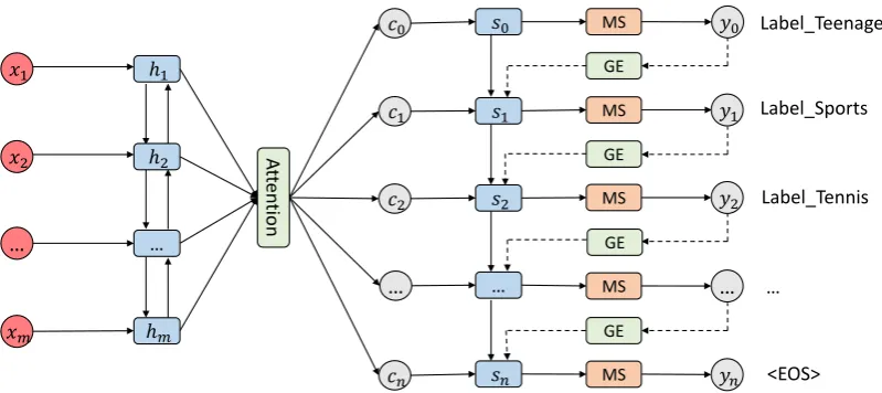
An overview of our proposed model is shown in Figure 1. First, we sort the label sequence of each sample according to the frequency of the labels in the training set. High-frequency labels are placed in the front. In addition, the bosand eos symbols are added to the head and tail of the label sequence, respectively.

The text sequence xis encoded to the the hidden states, which are aggregated to a context vector

ct by the attention mechanism at time-stept. The decoder takes the context vectorct, the last hidden statest−1 of the decoder and the embedding vectorg(yt−1) as the inputs to produce the hidden state stat time-stept. Hereyt−1 is the predicted probability distribution over the label spaceLat time-step t−1. The functiongtakesyt−1as input and produces the embedding vector which is then passed to the

decoder. Finally, the masked softmax layer is used to output the probability distributionyt.

2.2 Sequence Generation

MS 𝑠1 𝑠2 … MS GE GE MS 𝑐0 𝑐1

𝑠0 MS 𝑦0

GE

𝑐2

…

𝑐𝑛 𝑠𝑛 MS

𝑦2 … 𝑦𝑛 𝑦1 GE 𝑥1 𝑥2 𝑥𝑚 … ℎ𝑚 … ℎ2 ℎ1 A tten tion Label_Teenager Label_Sports Label_Tennis … <EOS>

Figure 1: The overview of our proposed model. MS denotes the masked softmax layer. GE denotes the global embedding.

Encoder:Let(w1,w2,· · ·,wm)be a sentence withmwords andwiis the one-hot representation of thei-th word. We first embedwito a dense embedding vectorxi by an embedding matrixE ∈Rk×|V|. Here|V|is the size of the vocabulary, andkis the dimension of the embedding vector.

We use a bidirectional LSTM (Hochreiter and Schmidhuber, 1997) to read the text sequencexfrom both directions and compute the hidden states for each word,

− →

hi =

−−−−→

LSTM(−→hi−1,xi) (2)

←− hi =

←−−−−

LSTM(←h−i+1,xi) (3)

We obtain the final hidden representation of the i-th word by concatenating the hidden states from both directions,hi = [

− →

hi;

←−

hi], which embodies the information of the sequence centered around the

i-th word.

Attention: When the model predicts different labels, not all text words make the same contribution. The attention mechanism produces a context vector by focusing on different portions of the text se-quence and aggregating the hidden representations of those informative words. Specially, the attention mechanism assigns the weightαtito thei-th word at time-steptas follows:

eti=vaT tanh(Wast+Uahi) (4)

αti=

exp(eti)

Pm

j=1exp(etj)

(5)

whereWa,Ua,vaare weight parameters andstis the current hidden state of the decoder at time-stept. For simplicity, all bias terms are omitted in this paper. The final context vectorctwhich is passed to the decoder at time-steptis calculated as follows:

ct= m

X

i=1

αtihi (6)

Decoder:The hidden statestof the decoder at time-steptis computed as follows:

st= LSTM(st−1,[g(yt−1);ct−1]) (7)

where[g(yt−1);ct−1]means the concatenation of the vectorsg(yt−1)andct−1. g(yt−1)is the

distribution over the label spaceLat time-stept−1and is computed as follows:

ot=Wof(Wdst+Vdct) (8)

yt=sof tmax(ot+It) (9)

whereWo,Wd, andVdare weight parameters,It ∈ RLis the mask vector that is used to prevent the decoder from predicting repeated labels, andf is a nonlinear activation function.

(It)i=

(

−∞ if the labellihas been predicted at previoust−1time steps.

0 otherwise. (10)

At the training stage, the loss function is the cross-entropy loss function. We employ the beam search algorithm (Wiseman and Rush, 2016) to find the top-ranked prediction path at inference time. The prediction paths ending with theeosare added to the candidate path set.

2.3 Global Embedding

In the sequence generation model mentioned above, the embedding vectorg(yt−1)in Equation (7) is the

embedding of the label that has the highest probability under the distributionyt−1. However, this

calcu-lation only takes advantage of the maximum value ofyt−1 greedily. The proposed sequence generation

model generates labels sequentially and predicts the next label conditioned on its previously predicted labels. Therefore, it is likely that we would get a succession of wrong label predictions in the following time steps if the prediction is wrong at time-stept, which is also calledexposure bias. To a certain extent, the beam search algorithm alleviates this problem. However, it can not fundamentally solve the problem because the exposure biasphenomenon is likely to occur for all candidate paths. yt−1 represents the

predicted probability distribution at time-stept−1, so it is obvious that all information inyt−1is helpful

when we predict the current label at time-step t. The exposure bias problem ought to be relieved by considering all informative signals contained inyt−1.

Based on this motivation, we propose a new decoder structure, where the embedding vectorg(yt−1)at

time-steptis capable of representing the overall information at(t−1)-th time step. Inspired by the idea of the adaptive gate in highway network (Srivastava et al., 2015), here we introduce our global embedding. Letedenotes the embedding of the label which has the highest probability under the distributionyt−1. ¯

eis the weighted average embedding at timet, which is calculated as follows:

¯ e=

L

X

i=1

y_t(i₋)₁ei (11)

wherey_t(₋i)₁is thei-th element ofyt−1andeiis the embedding vector of thei-th label. Then the proposed global embeddingg(yt−1)passed to the decoder at time-steptis as follows:

g(yt−1) = (1−H)e+He¯ (12)

whereH is the transform gate controlling the proportion of the weighted average embedding:

H =W1e+W2e¯ (13)

whereW1,W2 ∈RL×Lare weight matrices. The global embeddingg(yt−1)is the optimized

combina-tion of the original embedding and the weighted average embedding by using transform gateH, which can automatically determine the combination factor in each dimension. yt−1 contains the information

Dataset Total Samples Label Sets Words/Sample Labels/Sample

RCV1-V2 804,414 103 123.94 3.24 AAPD 55,840 54 163.42 2.41

Table 1: Summary of datasets. Total Samples, Label Sets denote the total number of samples and labels, respectively. Words/Sampleis the average number of words per sample andLabels/Sampleis the average number of labels per sample.

3 Experiments

In this section, we evaluate our proposed methods on two datasets. We first introduce the datasets, evaluation metrics, experimental details, and all baselines. Then, we compare our methods with the baselines. Finally, we provide the analysis and discussions of experimental results.

3.1 Datasets

Reuters Corpus Volume I (RCV1-V2)2: This dataset is provided by Lewis et al. (2004). It consists of over800,000manually categorized newswire stories made available by Reuters Ltd for research pur-poses. Multiple topics can be assigned to each newswire story and there are 103 topics in total.

Arxiv Academic Paper Dataset (AAPD)3:We build a new large dataset for the multi-label text classifi-cation. We collect the abstract and the corresponding subjects of55,840papers in the computer science field from the website4. An academic paper may have multiple subjects and there are 54 subjects in total. The target is to predict corresponding subjects of an academic paper according to the content of the abstract.

We divide each dataset into training, validation and test sets. The statistics of the two datasets are shown in Table 1.

3.2 Evaluation Metrics

Following the previous work (Zhang and Zhou, 2007; Chen et al., 2017), we adopt hamming loss and micro-F1 score as our main evaluation metrics. Micro-precision and micro-recall are also reported to

assist the analysis.

• Hamming-loss(Schapire and Singer, 1999) evaluates the fraction of misclassified instance-label pairs, where a relevant label is missed or an irrelevant is predicted.

• Micro-F1 (Manning et al., 2008) can be interpreted as a weighted average of the precision and

re-call. It is calculated globally by counting the total true positives, false negatives, and false positives.

3.3 Details

We extract the vocabularies from the training sets. For the RCV1-V2 dataset, the size of the vocabulary is50,000and out-of-vocabulary (OOV) words are replaced withunk. Each document is truncated at the length of 500 and the beam size is 5 at the inference stage. Besides, we set the word embedding size to 512. The hidden sizes of the encoder and the decoder are 256 and 512, respectively. The number of LSTM layers of encoder and decoder is 2.

For the AAPD dataset, the size of word embedding is 256. There are two LSTM layers in the encoder and its size is 256. For the decoder, there is one LSTM layer of size 512. The size of the vocabulary is 30,000and OOV words are also replaced withunk. Each document is truncated at the length of 500. The beam size is 9 at the inference stage.

We use the Adam (Kingma and Ba, 2014) optimization method to minimize the cross-entropy loss over the training data. For the hyper-parameters of the Adam optimizer, we set the learning rateα = 0.001, two momentum parameters β1 = 0.9andβ2 = 0.999respectively, and = 1×10−8. Additionally,

2_{http://www.ai.mit.edu/projects/jmlr/papers/volume5/lewis04a/lyrl2004_rcv1v2_}

README.htm 3

Models HL(-) P(+) R(+) F1(+)

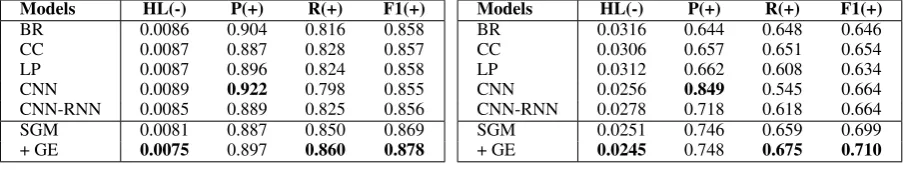
BR 0.0086 0.904 0.816 0.858 CC 0.0087 0.887 0.828 0.857 LP 0.0087 0.896 0.824 0.858 CNN 0.0089 0.922 0.798 0.855 CNN-RNN 0.0085 0.889 0.825 0.856 SGM 0.0081 0.887 0.850 0.869

+ GE 0.0075 0.897 0.860 0.878

(a) Performance on the RCV1-V2 test set.

Models HL(-) P(+) R(+) F1(+)

BR 0.0316 0.644 0.648 0.646 CC 0.0306 0.657 0.651 0.654 LP 0.0312 0.662 0.608 0.634 CNN 0.0256 0.849 0.545 0.664 CNN-RNN 0.0278 0.718 0.618 0.664 SGM 0.0251 0.746 0.659 0.699

+ GE 0.0245 0.748 0.675 0.710

(b) Performance on the AAPD test set.

Table 2: Comparison between our methods and all baselines on two datasets. GE denotes the global embedding. HL, P, R, and F1 denote hamming loss, micro-precision, micro-recall, and micro-F1,

re-spectively. The symbol “+” indicates that the higher the value is, the better the model performs. The symbol “-” is the opposite.

we make use of the dropout regularization (Srivastava et al., 2014) to avoid overfitting and clip the gradients (Pascanu et al., 2013) to the maximum norm of 10.0. During training, we train the model for a fixed number of epochs and monitor its performance on the validation set. Once the training is finished, we select the model with the best micro-F1score on the validation set as our final model and evaluate its

performance on the test set.

3.4 Baselines

We compare our proposed methods with the following baselines:

• Binary Relevance (BR)(Boutell et al., 2004) transforms the MLC task into multiple single-label classification problems by ignoring the correlations between labels.

• Classifier Chains (CC)(Read et al., 2011) transforms the MLC task into a chain of binary classifi-cation problems and takes high-order label correlations into consideration.

• Label Powerset (LP)(Tsoumakas and Katakis, 2006) transforms a label problem to a multi-class problem with one multi-multi-class multi-classifier trained on all unique label combinations.

• CNN (Kim, 2014) uses multiple convolution kernels to extract text features, which are then in-putted to the linear transformation layer followed by a sigmoid function to output the probability distribution over the label space. The multi-label soft margin loss is optimized.

• CNN-RNN(Chen et al., 2017) utilizes CNN and RNN to capture both the global and local textual semantics and model the label correlations.

Following the previous work (Chen et al., 2017), we adopt the linear SVM as the base classifier in BR, CC and LP. We implement BR, CC and LP by means of Scikit-Multilearn (Szyma´nski, 2017), an open-source library for the MLC task. We tune hyper-parameters of all baseline algorithms on the validation set based on the micro-F1score. In addition, training strategies mentioned in Zhang and Wallace (2015)

are used to tune hyper-parameters for the baselines CNN and CNN-RNN.

3.5 Results

For the purpose of simplicity, we denote the proposed sequence generation model asSGM. We report the evaluation results of our methods and all baselines on the test sets.

The experimental results of our methods and the baselines on dataset RCV1-V2 are shown in Table 2a. Results show that our proposed methods give the best performance in the main evaluation metrics. Our proposed SGM model using global embedding achieves a reduction of 12.79% hamming-loss and an improvement of 2.33% micro-F1 score over the most commonly used baseline BR. Besides, our

0 0.2 0.4 0.6 0.8 1

λ

7.4 7.6 7.8 8

8.2 ×10-3Hamming loss(-)

0 0.2 0.4 0.6 0.8 1

λ

0.865 0.87 0.875

0.88 F1(+)

Figure 2: The performance of the SGM model when using differentλ. The red dotted line represents the results of using the adaptive gate. The symbol “+” indicates that the higher the value is, the better the model performs. The symbol “-” is the opposite.

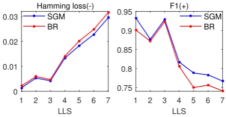
1 2 3 4 5 6 7 LLS

0 0.01 0.02 0.03

Hamming loss(-) SGM BR

1 2 3 4 5 6 7 LLS

0.75 0.8 0.85 0.9

0.95 F1(+) _SGM BR

Figure 3: The performance of the SGM model on different subsets of the RCV1-V2 test set. LLS rep-resents the length of label sequence of each sample in the subset. The explanations of symbol “+” and “-” can be found in Figure 2.

of 2.69% micro-F1 score over the traditional CNN model. Even without the global embedding, our

proposed SGM model is still able to outperform all baselines.

In addition, the SGM model is significantly improved by using global embedding. The SGM model with global embedding achieves a reduction of 7.41% hamming loss and an improvement of 1.04% micro-F1score on the test set compared with the model without global embedding.

Table 2b presents the results of the proposed methods and the baselines on the AAPD test set. Similar to the experimental results on the RCV1-V2 test set, our proposed methods still outperform all baselines by a large margin in main evaluation metrics. This further confirms that our methods have significant advantages over previous work on large datasets. Besides, the proposed SGM achieves a reduction of 2.39% hamming loss and an improvement of 1.57% micro-F1 score on the test set by using global

embedding. This further testifies that the global embedding is capable of helping the model to predict label sequences more accurately.

3.6 Analysis and Discussion

Here we perform further analysis on the model and experimental results. We report the evaluation results in terms of hamming loss and micro-F1 score.

3.6.1 Exploration of Global Embedding

As is shown in Table 2, global embedding can significantly improve the performance of the model. The global embeddingg(yt−1)at time-stepttakes advantage of all information of possible labels contained

inyt−1, so it is able to enrich the source information when the model predicts the current label, which

leads to the performance of the model significantly improved. The global embedding is the combination of original embeddingeand the weighted average embeddinge¯by using the transform gateH. Here we conduct experiments on the RCV1-V2 dataset to explore how the performance of our model is affected by the proportion between two kinds of embeddings. In the exploratory experiment, the final embedding vector at time-steptis calculated as follows:

g(yt−1) = (1−λ)∗e+λ∗e¯ (14)

The proportion between two kinds of embeddings is controlled by coefficientλ. λ = 0denotes the proposed SGM model without global embedding. The proportion of weighted average embedding in-creases when we increaseλ. The experimental results using differentλvalues in the decoder are shown in Figure 2.

As is shown in Figure 2, the performance of the model varies when different λ is used. Overall, the model using the adaptive gate performs the best, which achieves the best results in both hamming loss and micro-F1. The models withλ 6= 0outperform the model withλ = 0, which shows that the

Models HL(-) F1(+)

SGM 0.0081 0.869 w/o mask 0.0083(↓2.47%) 0.866(↓0.35%) w/o sorting 0.0084(↓3.70%) 0.858(↓1.27%)

(a) Ablation study for the SGM model.

Models HL(-) F1(+)

SGM + GE 0.0075 0.878 w/o mask 0.0078(↓4.00%) 0.873(↓0.57%) w/o sorting 0.0083(↓10.67%) 0.859(↓2.16%)

(b) Ablation study for SGM model with global embedding.

Table 3: Ablation study on the RCV1-V2 test set. GE denotes the global embedding. HL and F1 denote hamming loss and micro-F1, respectively. The symbol “+” indicates that the higher the value is, the

better the model performs. The symbol “-” is the opposite. ↑means that the performance of the model improves and↓is the opposite.

of the model. Without using the adaptive gate, the performance of the model improves at first and then deteriorates as λincreases. It reveals the reason why the model with the adaptive gate performs the best: the adaptive gate can automatically determine the most appropriateλvalue according to the actual condition.

3.6.2 The Impact of Mask and Sorting

Our proposed methods are developed based on traditional Seq2Seq models. However, the mask module is added to the proposed methods, which is used to prevent the models from predicting repeated labels. In addition, we sort the label sequence of each sample according to the frequency of appearance of labels in the training set. In order to explore the impact of the mask module and sorting, we conduct ablation experiments on the RCV1-V2 dataset. The experimental results are shown in Table 3. “w/o mask” means that we do not perform mask operation and “w/o sorting” means that we randomly shuffle the label sequence in order to perturb its original order.

As is shown in Table 3, the performance decline of the SGM model with global embedding is more significant compared with that of the SGM model without global embedding. In addition, the decline in the performance of the two models is more significant when we randomly shuffle the label sequence of the sample compared with removing mask module. The label cardinality of the RCV1-V2 dataset is small, so our proposed methods are less prone to predicting repeated labels. This explains the reason why experimental results indicate that the mask module has little impact on the models’ performance. In addition, the proposed models are trained using the maximum likelihood estimation method and the cross-entropy loss function, which requires humans to predefine the order of the output labels. Therefore, the sorting of labels is very important for the models’ performance. Besides, the performance of both models declines when we do not use the mask module. This shows that the performance of the model can be improved by using the mask operation.

3.6.3 Error Analysis

In the experiment, we find that the performance of all methods deteriorates when the length of the label sequence increases (for simplicity, we denote the length of the label sequence asLLS). In order to explore the influence of the value of theLLS, we divide the test set into different subsets based on differentLLS. Figure 3 shows the performance of the SGM model and the most commonly used baseline BR on different subsets of the RCV1-V2 test set. As is shown in Figure 3, generally, the performance of both models deteriorates as theLLSincreases. This shows that when the label sequence of the sample is particularly long, it is difficult to accurately predict all labels. Because more information is needed when the model predicts more labels. It is easy to ignore some true labels whose feature information is insufficient.

•Generating descriptions for videos has many ap-plications including human robot interaction.

•Many methods for image captioning rely on pre-trained object classifier CNN and Long Short Term Memory recurrent networks.

•How to learn robust visual classifiers from the weak annotations of the sentence descriptions.

(a) Visual analysis when the SGM model predicts “CV”.

•Generating descriptions for videos has many ap-plications including human robot interaction.

•Many methods for image captioning rely on pre-trained object classifier CNN and Long Short Term Memory recurrent networks.

•How to learn robust visual classifiers from the weak annotations of the sentence descriptions.

(b) Visual analysis when the SGM model predicts “CL”.

Table 4: An example abstract in the AAPD dataset, from which we extract three informative sentences. This abstract is assigned two labels: “CV” and “CL”. They denote computer vision and computational language, respectively.

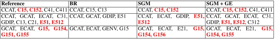
Reference BR SGM SGM + GE

CCAT,C15, C152, C41, C411 CCAT, C15, C13 CCAT,C15, C152 CCAT,C15, C152, C41, C411 CCAT, GCAT, ECAT, C31,

GDIP, C13, C21,E51, E512

CCAT, GCAT, GDIP, E51 CCAT, ECAT, GDIP, E51, E512

CCAT, GCAT, ECAT, C31, GDIP,E51, E512, C312 GCAT, ECAT, G15, G154,

G151, G155

GCAT, ECAT, GENV, G15 GCAT, ECAT, E21, G15, G154, G156

GCAT, ECAT, E21, G15, G154, G155

Table 5: Several examples of the generated label sequences on the RCV1-V2 dataset. The red bold labels in each example indicate that they are highly correlated.

3.6.4 Visualization of Attention

When the model predicts different labels, there exist differences in the contributions of different words. The SGM model is able to select the most informative words by utilizing the attention mechanism. The visualization of the attention layer is shown in Table 4. According to Table 4, when the SGM model predicts the label “CV”, it can automatically assign larger weights to more informative words, likeimage,visual,captioning, and so on. For the label “CL”, the selected informative words are sentence,memory,recurrent, etc. This shows that our proposed models are able to consider the differences in the contributions of textual content when predicting different labels and select the most informative words automatically.

3.6.5 Case Study

We give several examples of the generated label sequences on the RCV1-V2 dataset in Table 5, where we compare the proposed methods with the most commonly used baseline BR. The red bold labels in each example indicate that they are highly correlated. For instance, the correlation coefficient between E51 and E512 is 0.7664. Therefore, these highly correlated labels are likely to appear together in the predicted label sequence. The BR algorithm fails to capture this label correlation, leaving many true labels unpredicted. However, our proposed methods accurately predict almost all highly correlated true labels. The proposed SGM captures the correlations between labels by utilizing LSTM to generate la-bels sequentially. Therefore, for some true lala-bels whose feature information is insufficient, the proposed SGM is still able to generate them by considering relevant labels that have been predicted. In addition, label sequences that are more accurate are predicted by using global embedding. The SGM model with global embedding predicts more true labels compared with the SGM model without global embedding. The reason is that the source information is further enriched by incorporating overall informative signals in the probability distribution yt−1 when the model predicts the label at time-stept. Enriched

infor-mation makes global embedding more smooth, which enables the model to reduce damage caused by mispredictions made in the previous time steps.

4 Related Work

Problem transformation methods map the MLC task into multiple single-label learning tasks. Binary relevance (BR) (Boutell et al., 2004) decomposes the MLC task into independent binary classification problems by ignoring the correlations between labels. In order to model label correlations, label power-set (LP) (Tsoumakas and Katakis, 2006) transforms a multi-label problem to a multi-class problem with a classifier trained on all unique label combinations. Classifier chains (CC) (Read et al., 2011) trans-forms the MLC task into a chain of binary classification problems, where subsequent binary classifiers in the chain are built upon the predictions of preceding ones. However, the computational efficiency and performance of these methods are challenged by applications with a large number of labels and samples. Algorithm adaptation methods extend specific learning algorithms to handle multi-label data directly. Clare and King (2001) construct decision tree based on multi-label entropy to perform classification. Elisseeff and Weston (2002) optimize the empirical ranking loss by using maximum margin strategy and kernel tricks. Collective multi-label classifier (CML) (Ghamrawi and McCallum, 2005) adopts maximum entropy principle to deal with multi-label data by encoding label correlations as constraint conditions. Zhang and Zhou (2007) adoptk-nearest neighbor techniques to deal with multi-label data. F¨urnkranz et al. (2008) make ranking among labels by utilizing pairwise comparison. Li et al. (2015) propose a novel joint learning algorithm that allows the feedbacks to be propagated from the classifiers for latter labels to the classifier for the current label. Most methods, however, can only be used to capture the first or second order label correlations or are computationally intractable in considering high-order label correlations.

Among ensemble methods, Tsoumakas et al. (2011) break the initial set of labels into a number of small random subsets and employ the LP algorithm to train a corresponding classifier. Szyma´nski et al. (2016) propose to construct a label co-occurrence graph and perform community detection to partition the label set.

In recent years, some neural network models have also been used for the MLC task. Zhang and Zhou (2006) propose the BP-MLL that utilizes a fully-connected neural network and a pairwise ranking loss function. Nam et al. (2013) propose a neural network using cross-entropy loss instead of ranking loss. Benites and Sapozhnikova (2015) increase classification speed by adding an extra ART layer for cluster-ing. Kurata et al. (2016) utilize word embeddings based on CNN to capture label correlations. Chen et al. (2017) propose to represent semantic information of text and model high-order label correlations by combining CNN with RNN. Baker and Korhonen (2017) initialize the final hidden layer with rows that map to co-occurrence of labels based on the CNN architecture to improve the performance of the model. Ma et al. (2018) propose to use the multi-label classification algorithm for machine translation to handle the situation where a sentence can be translated into more than one correct sentences.

5 Conclusions and Future Work

In this paper, we propose to view the multi-label classification task as a sequence generation problem to model the correlations between labels. A sequence generation model with a novel decoder structure is proposed to improve the performance of classification. Extensive experimental results show that the proposed methods outperform the baselines by a substantial margin. Further analysis of experimental results demonstrates that our proposed methods not only capture the correlations between labels, but also select the most informative words automatically when predicting different labels.

As analyzed in Section 3.6.3, when a large number of labels are assigned to a sample, how to predict all these true labels accurately is an intractable problem. Our proposed methods alleviate this problem to some extent, but more effective solutions need to be further explored in the future.

6 Acknowledgements

References

Dzmitry Bahdanau, Kyunghyun Cho, and Yoshua Bengio. 2014. Neural machine translation by jointly learning to align and translate. CoRR, abs/1409.0473.

Simon Baker and Anna Korhonen. 2017. Initializing neural networks for hierarchical multi-label text classifica-tion. InBioNLP.

Fernando Benites and Elena Sapozhnikova. 2015. Haram: a hierarchical aram neural network for large-scale text classification. InData Mining Workshop (ICDMW), 2015 IEEE International Conference on, pages 847–854. IEEE.

Matthew R. Boutell, Jiebo Luo, Xipeng Shen, and Christopher M. Brown. 2004. Learning multi-label scene classification. Pattern Recognition, 37(9):1757–1771.

Guibin Chen, Deheng Ye, Zhenchang Xing, Jieshan Chen, and Erik Cambria. 2017. Ensemble application of convolutional and recurrent neural networks for multi-label text categorization. In 2017 International Joint Conference on Neural Networks, IJCNN 2017, Anchorage, AK, USA, May 14-19, 2017, pages 2377–2383.

Amanda Clare and Ross D King. 2001. Knowledge discovery in multi-label phenotype data. InEuropean Con-ference on Principles of Data Mining and Knowledge Discovery, pages 42–53. Springer.

Andr´e Elisseeff and Jason Weston. 2002. A kernel method for multi-labelled classification. InAdvances in neural information processing systems, pages 681–687.

Johannes F¨urnkranz, Eyke H¨ullermeier, Eneldo Loza Menc´ıa, and Klaus Brinker. 2008. Multilabel classification via calibrated label ranking. Machine learning, 73(2):133–153.

Nadia Ghamrawi and Andrew McCallum. 2005. Collective multi-label classification. InProceedings of the 14th ACM international conference on Information and knowledge management, pages 195–200. ACM.

Siddharth Gopal and Yiming Yang. 2010. Multilabel classification with meta-level features. InProceedings of the 33rd international ACM SIGIR conference on Research and development in information retrieval, pages 315–322. ACM.

Sepp Hochreiter and J¨urgen Schmidhuber. 1997. Long short-term memory. Neural computation, 9(8):1735–1780.

Ioannis Katakis, Grigorios Tsoumakas, and Ioannis Vlahavas. 2008. Multilabel text classification for automated tag suggestion. InProceedings of the ECML/PKDD, volume 18.

Yoon Kim. 2014. Convolutional neural networks for sentence classification. InProceedings of the 2014 Confer-ence on Empirical Methods in Natural Language Processing, EMNLP 2014, October 25-29, 2014, Doha, Qatar, A meeting of SIGDAT, a Special Interest Group of the ACL, pages 1746–1751.

Diederik P. Kingma and Jimmy Ba. 2014. Adam: A method for stochastic optimization.CoRR, abs/1412.6980.

Gakuto Kurata, Bing Xiang, and Bowen Zhou. 2016. Improved neural network-based multi-label classification with better initialization leveraging label co-occurrence. InNAACL HLT 2016, The 2016 Conference of the North American Chapter of the Association for Computational Linguistics: Human Language Technologies, San Diego California, USA, June 12-17, 2016, pages 521–526.

David D. Lewis, Yiming Yang, Tony G. Rose, and Fan Li. 2004. RCV1: A new benchmark collection for text categorization research.Journal of Machine Learning Research, 5:361–397.

Li Li, Houfeng Wang, Xu Sun, Baobao Chang, Shi Zhao, and Lei Sha. 2015. Multi-label text categorization with joint learning predictions-as-features method. InProceedings of the 2015 Conference on Empirical Methods in Natural Language Processing, pages 835–839.

Junyang Lin, Xu Sun, Shuming Ma, and Qi Su. 2018. Global encoding for abstractive summarization. InACL 2018.

Minh-Thang Luong, Hieu Pham, and Christopher D. Manning. 2015. Effective approaches to attention-based neural machine translation. CoRR, abs/1508.04025.

Christopher D Manning, Prabhakar Raghavan, Hinrich Sch¨utze, et al. 2008. Introduction to information retrieval, volume 1. Cambridge university press Cambridge.

Jinseok Nam, Jungi Kim, Iryna Gurevych, and Johannes F¨urnkranz. 2013. Large-scale multi-label text classifica-tion - revisiting neural networks. CoRR, abs/1312.5419.

Razvan Pascanu, Tomas Mikolov, and Yoshua Bengio. 2013. On the difficulty of training recurrent neural net-works. InInternational Conference on Machine Learning, pages 1310–1318.

Jesse Read, Bernhard Pfahringer, Geoff Holmes, and Eibe Frank. 2011. Classifier chains for multi-label classifi-cation. Machine learning, 85(3):333.

Alexander M. Rush, Sumit Chopra, and Jason Weston. 2015. A neural attention model for abstractive sentence summarization. InProceedings of the 2015 Conference on Empirical Methods in Natural Language Processing, EMNLP 2015, Lisbon, Portugal, September 17-21, 2015, pages 379–389.

Robert E Schapire and Yoram Singer. 1999. Improved boosting algorithms using confidence-rated predictions. Machine learning, 37(3):297–336.

Robert E Schapire and Yoram Singer. 2000. Boostexter: A boosting-based system for text categorization.Machine learning, 39(2-3):135–168.

Tianxiao Shen, Tao Lei, Regina Barzilay, and Tommi S. Jaakkola. 2017. Style transfer from non-parallel text by cross-alignment. CoRR, abs/1705.09655.

Nitish Srivastava, Geoffrey E. Hinton, Alex Krizhevsky, Ilya Sutskever, and Ruslan Salakhutdinov. 2014. Dropout: a simple way to prevent neural networks from overfitting. Journal of Machine Learning Research, 15(1):1929– 1958.

Rupesh Kumar Srivastava, Klaus Greff, and J¨urgen Schmidhuber. 2015. Highway networks. CoRR, abs/1505.00387.

Xu Sun, Bingzhen Wei, Xuancheng Ren, and Shuming Ma. 2017. Label embedding network: Learning label representation for soft training of deep networks. CoRR, abs/1710.10393.

Piotr Szyma´nski, Tomasz Kajdanowicz, and Kristian Kersting. 2016. How is a data-driven approach better than random choice in label space division for multi-label classification? Entropy, 18(8):282.

Piotr Szyma´nski. 2017. A scikit-based python environment for performing multi-label classification. arXiv preprint arXiv:1702.01460.

Grigorios Tsoumakas and Ioannis Katakis. 2006. Multi-label classification: An overview. International Journal of Data Warehousing and Mining, 3(3).

Grigorios Tsoumakas, Ioannis Katakis, and Ioannis Vlahavas. 2011. Random k-labelsets for multilabel classifica-tion. IEEE Transactions on Knowledge and Data Engineering, 23(7):1079–1089.

Sam Wiseman and Alexander M. Rush. 2016. Sequence-to-sequence learning as beam-search optimization. CoRR, abs/1606.02960.

Jingjing Xu, Xu Sun, Qi Zeng, Xuancheng Ren, Xiaodong Zhang, Houfeng Wang, and Wenjie Li. 2018. Unpaired sentiment-to-sentiment translation: A cycled reinforcement learning approach. ACL 2018.

Ye Zhang and Byron C. Wallace. 2015. A sensitivity analysis of (and practitioners’ guide to) convolutional neural networks for sentence classification. CoRR, abs/1510.03820.

Min-Ling Zhang and Zhi-Hua Zhou. 2006. Multilabel neural networks with applications to functional genomics and text categorization. IEEE Transactions on Knowledge and Data Engineering, 18(10):1338–1351.