98
Noise and Performance Analysis of Image compression
by Hybrid technique
(Neural Network combined with DWT)
Mr.Murali Mohan.S
1, Dr. P.Satyanarayana
2Associate Professor 1, Professor2 ,
Dept. of ECE, SVCET, Chittoor,A.P.,INDIA1 , College of Engineering, S.V.University, Tirupathi, A.P., INDIA2. Email: [email protected], [email protected]
In signal and image processing techniques for pattern recognition and template matching Neural networks are significantly used. In this work image compression is done by neural networks. DWT is combined with NN for achieving better MSE and increase in compression ration greater than 100%. NN architecture achieves maximum of 98% with use of four neurons in the hidden layer, with selection of LL sub band only the compression is improved by another 75%. The design proposed is suitable for high resolution image compression to improve the performance of image compression algorithm.
Index Terms- DWT, Neural Network, Image Compression, Hybrid technique, MSE, Daubechies and Haar wavelet filters, tansig and purelin functions.
1. INTRODUCTION
Image compression is one of the most promising subjects in image processing. Images captured need to be stored or transmitted over long distances. Raw image occupies memory and hence need to be compressed. With the demand for high quality video on mobile platforms there is a need to compress raw images and reproduce the images without any degradation. Several standards such as JPEG200, MPEG-2/4 recommend use of Discrete Wavelet Transforms (DWT) for image transformation [1] which leads to compression with when encoded. Wavelets are a mathematical tool for hierarchically decomposing functions in multiple hierarchical sub bands with time scale resolutions. Image compression using Wavelet Transforms is a powerful method that is preferred by scientists to get the compressed images at higher compression ratios with higher PSNR values [2]. It is a popular transform used for some of the image compression standards in lossy compression methods. Unlike the discrete cosine transform, the wavelet transform is not Fourier-based and therefore wavelets do a better job of handling discontinuities in data.
On the other hand, Artificial Neural Networks (ANN) for image compression applications has marginally increased in recent years. Neural networks are inherent adaptive systems [3][4][5][6]; they are suitable for handling nonstationaries in image data. Artificial neural network can be employed with success to image compression. Image Compression Using Neural Networks by Ivan Vilovic [7] reveals a direct solution method for image compression using the neural networks. An experience of using multilayer perceptron for image compression is also presented. The multilayer perceptron is
99
data achieved by such a representation of WN’s. Zhang [15]has proved that the WN’s can manipulate the non-linear regression of the moderately big dimension of entry with the data of training. Ramanaiah and Cyril [16] in their paper have reported the use of neural networks and wavelets for image compression. In their work, the image is decomposed using DWT into four sub bands, and the neural network compresses the individual sub band and hence blocking artifacts error is minimized in the reconstructed image. Image decomposition using DWT into multiple sub bands leads to delay in compression, as the decomposition of image leads to multiple hierarchical sub blocks. In this paper we propose a novel approach for image compression using wavelets and neural networks. The input image is decomposed into four sub bands of LL, LH, HL and HH. Only the LL sub band is further decomposed in hierarchical sub bands until the sub band size is 8 x 8. The sub bands after decomposition using DWT are chosen based on information content and is further compressed using multilayered neural network architecture, thus minimizing the delay in compression.
Section II presents theoretical background on neural networks and DWT. Section III discusses the proposed image compression technique, section IV discusses the results and conclusion is presented in section V.
2. NEURAL NETWORKS AND DWT
In this section, neural network architecture for image compression is discussed. Feed forward neural network architecture and back propagation algorithm for training is presented. DWT based image transformation and compression is also presented in this section. Compression is one of the major subject of research, the need for compression is discussed as follows: Uncompressed video of size 640 x 480 resolution, with each pixel of 8 bit (1 bytes), with 24 fps occupies 307.2 Kbytes per image (frame) or 7.37 Mbytes per second or 442 Mbytes per minute or 26.5 Gbytes per hour. If the frame rate is increased from 24 fps to 30 fps, then for 640 x 480 resolution, 24 bit (3 bytes) colour, 30 fps occupies 921.6 Kbytes per image (frame) or 27.6 Mbytes per second or 1.66 Gbytes per minute or 99.5 Gbytes per hour. Given a 100 Gigabyte disk can store about 1-4 hours of high quality video, With channel data rate of 64Kbits/sec – 40 – 438 secs/per frame transmission. For HDTV with 720 x 1280 pixels/frame, progressive scanning at 60 frames/s: 1.3Gb/s – with 20Mb/s available – 70% compression required – 0.35bpp. In this work we propose a novel architecture based on neural network and DWT.
2.1. Feed forward neural network architecture for image compression
An Artificial Neural Network (ANN) is an information- processing paradigm that is inspired by the way biological nervous systems, such as the Brian, process information [16].
The key element of this paradigm is the novel structure of the information processing system. The basic architecture for image compression using neural network is shown in figure 1. The network has input layer, hidden layer and output layer. Inputs from the image are fed into the network, which are passed through the multi layered neural network. The input to the network is the original image and the output obtained is the reconstructed image. The output obtained at the hidden layer is the compressed image. The network is used for image compression by breaking it in two parts as shown in the Fig. 1. The transmitter encodes and then transmits the output of the hidden layer (only 16 values as compared to the 64 values of the original image). The receiver receives and decodes the 16 hidden outputs and generates the 64 outputs. Since the network is implementing an identity map, the output at the receiver is an exact reconstruction of the original image.
Fig. 1 Feed forward multilayered neural network architecture [17]
Three layers, one input layer, one output layer and one hidden layer, are designed. The input layer and output layer are fully connected to the hidden layer. Compression is achieved by designing the network such that the number of neurons at the hidden layer is less than that of neurons at both input and the output layers. The input image is split up into blocks or vectors of 8 X8, 4 X 4 or 16 X 16 pixels.
Back-propagation is one of the neural networks which are directly applied to image compression coding [18][19][20]. In the previous sections theory on the basic structure of the neuron was considered. The essence of the neural networks lies in the way the weights are updated. The updating of the weights is through a definite algorithm. In this paper Back Propagation (BP) algorithm is studied and implemented. The algorithm is applied for the supervised learning that is a desired output will be applied to Neural Architecture. The target is represented as di (desired output) for the ith output
unit. The actual output of the layer is given by ai. Thus the
error or cost function is given by [21]
2 2
)
(
2
1
i
d
a
E
i
−
100
This process of computing the error is called a forward pass.How the output unit affects the error in the ith layer is given by differentiating equation 2.5 by ai
)
(
2 ii
d
a
a
E
i
−
=
∂
∂
2.6
The equation 2.6 can be written in the other form as
)
(
)
(
a
2id
id
a
2ii
=
−
∂
2.7where d(ai) is the differentiation of the ai. The weight update
is given by
1
i
a
i
ij
w
=
∂
∆
η
2.8Where a1i is the output of the hidden layer or input to the
output neuron and
η
is the learning rate [1]. This error has to propagate backwards from the output to the input. The∂
for the hidden layer is calculated asi ij r
hiddenlaye
=
d
a
iw
∂
∂
(
1)
∑
2.9Weight update for the hidden layer with new
∂
, will be done using equation 2.8. Equation 2.5 - 2.9 depend on the number of the neurons present in the layer and the number of layers present in the network.2.2. DWT architecture for image compression
[image:3.595.316.515.118.221.2]The DWT represents the signal in dynamic sub-band decomposition. Generation of the DWT in a wavelet packet allows sub-band analysis without the constraint of dynamic decomposition. The discrete wavelet packet transform (DWPT) performs an adaptive decomposition of frequency axis. The specific decomposition will be selected according to an optimization criterion. The Discrete Wavelet Transform (DWT), based on time-scale representation, provides efficient multi-resolution sub-band decomposition of signals. It has become a powerful tool for signal processing and finds numerous applications in various fields such as audio compression, pattern recognition, texture discrimination, computer graphics [22][23][24] etc. Specifically the 2-D DWT and its counterpart 2-D Inverse DWT (IDWT) play a significant role in many image/video coding applications. Fig. 2 shows the DWT architecture, the input image is decomposed into high pass and low pass components using HPF and LPF filters giving rise to the first level of hierarchy. The process is continued until multiple hierarchies are obtained. A1 and D1 are the approximation and detail filters.
Fig. 2 DWT decomposition
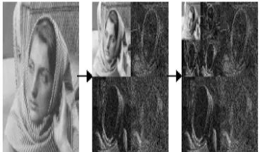
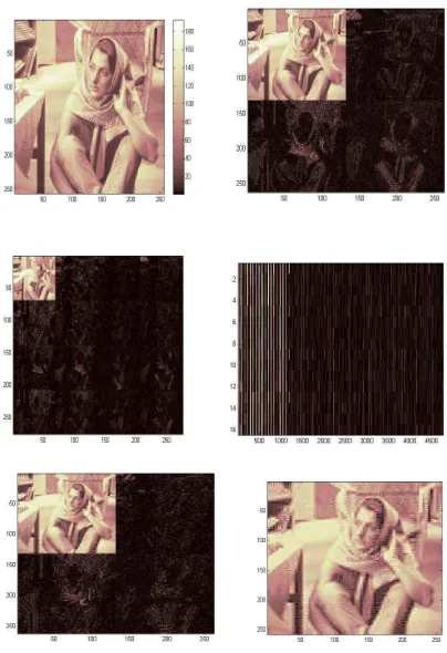
[image:3.595.335.519.361.469.2]Fig. 3 shows the decomposition results. The barbera image is first decomposed into four sub bands of LL, LH, HL and HH. Further the LL sub band is decomposed into four more sub bands as shown in the figure. The LL component has the maximum information content as shown in figure 3, the other higher order sub bands contain the edges in the vertical, horizontal and diagonal directions. An image of size N X N is decomposed to N/2 X N/2 of four sub bands. Choosing the LL sub band and rejecting the other sub bands at the first level compresses the image by 75%. Thus DWT assists in compression. Furhter encoding increases compression ratio.
Fig. 3 DWT decomposition of barbera image into hierarchical sub bands
3. ANN WITH DWT FOR IMAGE COMPRESSION
101
Fig. 4 Neural network based image compression
[image:4.595.306.556.250.355.2]Prior to use of NN for compression it is required to perform training of the network, in this work we have used back propagation training algorithm for obtaining the optimum weights and biases for the NN architecture. Based on the training, barbera image is compressed and decompressed; Fig. 5 shows the input image, compressed image and decompressed image.
Fig. 5 NN based image compression and decompression
Fig. 5 also shows the input image and the decompressed image of coins image using neural network architecture. From the decompressed results shown, we find the checker blocks error, which exists on the decompressed image. As the input image is sub divided into 8 x 8 blocks and rearranged to
64 x 1 input matrixes, the checker block arises. This is one of the limitations of NN based compression. Another major limitation is the maximum compression ration which is less than 100%, in order to achieve compression more than 100% and to eliminate checker box errors or blocking artifacts we proposed DWT combined with NN architecture for image compression.
3.1 Proposed Technique for Image Compression
Most of the image compression techniques use either neural networks for compression or DWT (Discrete wavelet Transform) based transformation for compression. In order to overc
ome the limitat ions of NN archit ecture in this work,
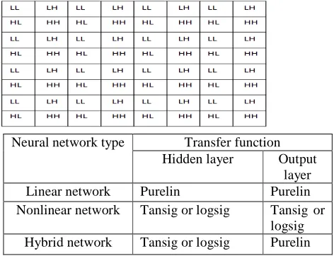
DWT is used for image decomposition and an N X N image is decomposed using DWT into hierarchical blocks the decomposition is carried out until the sub block is of size 8 x 8. For a image of size 64 x 64, first level decomposition gives rise to 32 x 32 (four sub bands) of sub blocks, further decomposition leads to 16 x 16 (sixteen sub bands), which can further decamped to 8 x 8 at the third hierarchy. The third level of hierarchy there are 64 sub blocks each of size 8 x 8. Figure 6 shows the decomposition levels of input image of size 64 x 64.
Network size
Size of hidden Layer
Compression Ratio
64-64-64 64 0%
64-32-64 32 50%
64-16-64 16 75%
64-08-64 08 87.5%
64-04-64 04 93.75%
64-01-64 01 98.5%
Neural network type Transfer function Hidden layer Output
layer Linear network Purelin Purelin Nonlinear network Tansig or logsig Tansig or
[image:4.595.62.275.474.647.2] [image:4.595.307.543.484.665.2]102
Fig. 6 Decomposition of image into sub blocks using DWT
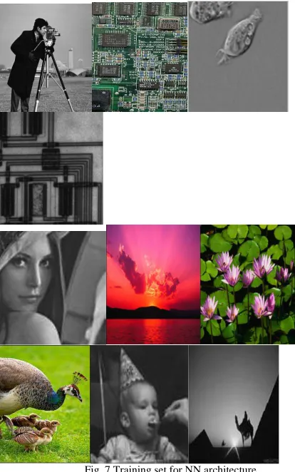
[image:5.595.49.256.328.659.2]Sub blocks of 8 x 8 are rearranged to 64 x 1 block are combined together into a rearranged matrix size as shown in fig. 6. The rearranged matrix is used to train the NN architecture based on back propagation algorithm. In order to train the NN architecture and to obtain optimum weights it is required to select appropriate images. The training vectors play a vital role in NN architecture for image compression. Fig. 7 shows the training sets for NN architecture.
Fig. 7 Training set for NN architecture
The NN architecture consisting of input layer, hidden layer and output layer. The hidden layer consists of network function of four types shown in Table 1. Similarly the output
layer also can be any of the four network functions. It is required to choose appropriate network function.
Table 1 Neural network classification based on transfer function
Trainrp is a network training function used in this work that updates weight and bias values according to the resilient backpropagation algorithm (Rprop). Trainlm may also be used which is also a network training function that updates weight and bias values according to Levenberg algorithm but consumes more memory.
3.2 Proposed hybrid architecture
[image:5.595.323.530.427.532.2]In this work, hybrid neural network architecture which combines DWT with NN is used to image compression. The hybrid architecture is discussed in [Ramanaiah and Cyril]. The NN based compression using analog VLSI is presented in [Cyril and Pinjare]. Based on the two different papers neural network architecture is developed and is trained to compress and decompress multiple images. The DWT based image compression algorithm is combined with neural network architecture. There are several wavelet filters and neural network functions. It is required to choose appropriate wavelets and appropriate neural network functions. In this work an experimental setup is modeled using Matlab to choose appropriate wavelet and appropriate neural network function. Based on the above parameters chosen the Hybrid Compression Algorithm is developed and is shown in Fig. 8.
Fig. 8 Proposed hybrid algorithms for image compression
103
output layer to decompress. The decompressed is furtherconverted from vector to blocks of sub bands. The sub band components are grouped together and are transformed using inverse DWT. The transformation is done using multiple hierarchies and the original image is reconstructed. The input image and the output image is used to compute MSE, PSNR. The selection of network parameters and performances are discussed in the next section.
4. RESULTS AND DISCUSSION
Training the network using the test training sets and selection of appropriate network function is carried out, Matlab model is developed and is used for analysis.
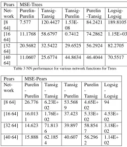
[image:6.595.306.563.119.240.2]Table 2 NN performance for various network functions for Pears
Table 3 NN performance for various network functions for Trees
Pears MSE-Pears Net-work Purelin -Purelin Tansig - Tansig Tansig - Purelin Purelin -Tansig Logsig -Logsig [8 64] 26.776 6.23E+
02 53.568 9 4.65E+ 02 94 [16 64] 16.013
1
1.76E+ 02
37.423 5.33E+ 02
[image:6.595.41.291.294.582.2]4.53E+ 02 [32 64] 14.623 71.813
6
39.897 58.854 7
[image:6.595.307.532.468.640.2]3.18E+ 02 [40 64] 15.888 62.185
4
40.607 56.296 2
1.14E+ 02 Table 2 and Table 3 shows the results for Pears image for various network functions and hidden layer size. From the results presented in Table 2 and Table 3 shows that for NN architecture of [8 64] (8 neurons in hidden layer and 64 in the output layer), MSE is very less for Tansig-Purelin. Hence in this work, we propose tansig and purelin are the network functions for NN architecture and are called as Hybrid NN architecture. Fig. 9 shows the MSE, PSNR and Max Error parameters for various input block size.
Fig. 9 Input block size and NN performance
From the results shown in fig. 9 it is found that lesser input layer size better is MSE, however if the input layer size less it also increases the complexity of NN architecture. Number of hierarchical levels in DWT need to be increased, hence in this work we choose 8 x 8 block size, the input image is divided into 8 x 8 block size using DWT. Fig. 10 shows the results of selection of number of hidden layers. The input layer consisting of 64 x 1 can be compressed to 16 x 1, which can be further compressed to 8 x 1, and further to 4 x 1 and can be reconstructed to 64 x 1 at the output layer. The results shown are analyzed for three images, from the results it is found that increasing the number of hidden layers does not improve NN compression performance. Hence the network chosen in this work consists of input layer of 64 x 1, hidden layer of 4 x 1 and output layer of 64 x 1. The network functions are tansig in the hidden layer and purelin in the output layer. 16:8:4:8:16 0 20 40 60 80 100 120
Trees Pears Peppers
Ima ge s
P e rf ro m a n c e p a ra m e te rs Max Error MSE PSNR 16:8:4:2:4:8:16 0 20 40 60 80 100 120 140 160 180 200
Trees Pears Peppers
Images P e rf ro m a n c e p a ra m e te rs Max Error MSE PSNR
Fig. 10 NN performances for various hidden layers
In this proposed architecture, the input image is first decomposed into multiple sub blocks using hierarchical DWT architecture, the decomposed image is reordered and is processed using the NN architecture. The NN architecture Pears MSE-Trees
Net-work Purelin-Purelin Tansig- Tansig Tansig- Purelin Purelin -Tansig Logsig-Logsig [8 64]
7.577 120.4427 1.53E-08
84.2421 189.8105 [16
64]
11.1768 58.6797 0.7412 74.2862 1.15E+03 [32
64]
20.5682 32.5422 29.6525 56.2924 82.2705 [40
64]
104
compresses the transformed image, appropriate weights andbiases are chosen for compression and decompression. Hybrid network functions are used for NN architecture. The decompressed image is reconstructed using IDWT. Fig. 11 shows the results of image compression and decompression using the proposed hybrid architecture model. The input image is transformed into four sub bands in the first level decomposition, further is decomposed to second level of hierarchy and is shown in fig. 11. The decomposed image is rearranged into column matrix, and is shown in fig. 11. The compressed data using NN architecture is decompressed using output layer. The output obtained is further rearranged to sub blocks and is inverse transformed using inverse DWT. The output obtained is shown in figure, along with the
[image:7.595.315.518.119.305.2]reconstructed image.
Fig. 11 Results of hybrid neural network architecture
Fig. 12 Input image and reconstructed image
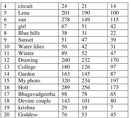
[image:7.595.55.257.286.581.2]Table 4 summarizes the MSE results for various test images using the hybrid architecture. The results compare the performances of NN architecture, reference design and the present work. With the choice of appropriate wavelet filters (Haar, db4), choice of decomposition levels, number of hidden layers and network function the proposed architecture is superior compared with all the other architectures.
Table 4 Comparison of proposed design with MSE results
Sl. No.
Test Image Image MSE (With NN only)
Reference Image MSE (With NN and DWT)
1 cameraman 321 301 262
2 board 1590 1289 958
[image:7.595.315.546.611.725.2]105
4 circuit 24 21 14
5 Lena 201 190 100
6 sun 278 149 115
7 girl 67 51 42
8 Blue hills 38 31 22
9 Sunset 51 47 39
10 Water lilies 56 42 31
11 Winter 89 52 47
12 Drawing 260 232 170
13 College 180 126 97
14 Garden 163 145 87
15 My photo 320 234 197
16 Holi 289 256 175
17 Bhagavadgeetha 98 78 65 18 Devine couple 143 101 80
19 krishna 29 19 7
20 Goddess 76 53 45
From the results presented in table 4 for all the 20 images considered proposed network achieves less MSE compared with the reference design. The input image is decomposed using DWT and is compressed using NN architecture, this introduces delay and hence high speed architectures are required to implement for real time applications.
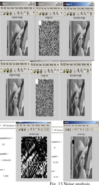
4.1 Noise Analysis
One of the major objectives of this work is to analyze the network performance under the influence of noise and error. Noisy image is given as input to the network, and the network performance is analyzed. Different noise sources such as Gaussian noise, Poisson noise and Salt & pepper noise with SNR of 10 dB are added to the image prior to compression and decompression. Error analysis is also carried out by introducing error in the compressed data.
Table 5 presents the MSE and PSNR results obtained for four images with 0.5 bpp and 1 bpp compression. The results are obtained on images of size 256 x 256. From the results obtained the following are the observations made:
1.Without noise hybrid neural network architecture and linear neural network architecture achieve better MSE and PSNR. With salt and pepper noise added to the image, MSE and PSNR achieved using DWT-SPIHT technique have large variations as compared with hybrid and linear neural network architectures.
2.Neural network technique (hybrid and linear) achieve good MSE and PSNR even when the image is corrupted with noise.
Table 5 Results of noise analysis (Salt and Pepper)
Bpp = 1, Salt & Pepper Noise Mean Square Error
Hybrid DWT-SPIHT
Without noise
With Noise
Without noise
With noise Baboon 619.07 687.93 868.21 1.40E+03 Testim 189.00 262.07 213.34 1.01E+03 Peppers 142.01 212.22 189.37 946.31 Image1 33.87 96.20 46.78 882.80
PSNR
Hybrid DWT-SPIHT
Without noise
With noise
Without noise
With noise Baboon 20.21 19.75 18.78 16.68 Testim 25.36 23.94 21.28 18.09 Peppers 26.60 24.86 24.53 18.37 Image1 32.83 28.29 22.61 18.67
Bpp = 0.5, Salt & Pepper Noise Mean Square Error
Hybrid DWT-SPIHT
Without noise
With Noise
Without noise
With noise Baboon 640.76 859.96 721.08 1.73E+03 Testim 177.60 438.96 194.90 1.44E+03 Peppers 139.74 383.19 145.50 1.20E+03 Image1 33.12 241.57 46.15 1.01E+03
PSNR
Hybrid DWT-SPIHT
Without noise
With noise
Without noise
[image:8.595.57.284.110.315.2]106
Fig. 13 Noise analysis
Test results for various noise sources have been demonstrated that the proposed network is suitable for compression and decompression of images over noisy channel.
5. CONCLUSION
Use of NN for image compression has superior advantage compared with classical techniques, however the NN architecture requires image to be decomposed to several blocks of each 8 x 8, and hence introduces blocking artifact errors and checker box errors in the reconstructed image. In order to overcome the checker errors in this work, we have used DWT for image decomposition prior to image compression using NN architecture. In this work, we proposed a hybrid architecture that combines NN with DWT and the input image is used to train the network. The network architecture is used to compress and decompress several image and it is proven to achieve better MSE compared with reference design. The hybrid technique uses hidden layer consisting of tansig function and output layer with purelin function to achieve better MSE. The proposed architecture is suitable for real time application of image compression and decompression.
References
[1] A. D’souza Winston and Tim Spracklen. Application of Artificial Neural
Networks for real time Data Compression, 8th International Conference On Neural Processing, Shanghai, Chine, 14-18 Novembre 2001. [2] A. Grossmann and B. Torrésani, Les ondelettes, Encyclopedia Universalis, 1998.
[3] A. Khashman and K. Dimililer, “Comparison Criteria for Optimum Image Compression”, Proceeding of the IEEE International Conference on ‘Computer as a Tool’ EUROCON’05, vol. 2, 2005, pp. 935-938. [4] C. Foucher and G. Vaucher. Compression d’images et réseaux de neurones, revue Valgo n°01-02, 17-19 octobre 2001, Ardèche.
[5] Ch. Bernard, S. Mallat and J-J Slotine. Wavelet Interpolation Networks, International Workshop on CAGD and wavelet methods for
Reconstructing Functions, Montecatini, 15-17 Juin 1998.
[6] D. Charalampidis. Novel Adaptive Image Compression, Workshop on Information and Systems Technology, Room 101, TRAC Building, University of New Orleans, 16 Mai 2003.
[7] G. Lekutai. Adaptive Self-tuning Neuro Wavelet Network Controllers, Thèse de Doctorat, Blacksburg-Virgina, Mars 1997.
[8]I. Vilovic, “An Experience in Image Compression Using Neural Networks”, 48th International Symposium ELMAR-2006 focused on
Multimedia Signal Processing and Communications, IEEE, 2006, pp. 95- 98.
[9] J. Jiang. Image compressing with neural networks – A survey, Signal processing: Image communication, ELSEVIER, vol. 14, n°9, 1999, pp. 737-760.
[10] K. H. Talukder and K. Harada, “Haar Wavelet Based Approach for Image Compression and Quality Assessment of Compressed Image”, IAENG International Journal of Applied Mathematics, 2007. [11] K. Ratakonda and N. Ahuja, “Lossless Image Compression with Multiscale Segmentation”, IEEE Transactions Image Processing, vol. 11, no.11, 2002, pp. 1228-1237.
[12] M. Chtourou. Les réseaux de neurones, Support de cours DEA A-II, Année Universitaire 2002/2003.
[13] M. J. Nadenau, J. Reichel, and M. Kunt, “Wavelet Based Color Image Compression: Exploiting the Contrast Sensitivity Function”, IEEE Transactions Image Processing, vol. 12, no.1, 2003, pp. 58-70. [14] Q. Zang and A. Benveniste, Wavelet networks. IEEE Trans. Neural Networks, vol. 3, pp. 889-898, 1992.
[15] Q. Zang, Wavelet Network in Nonparametric Estimation. IEEE Trans. Neural Networks, 8(2):227- 236, 1997.
[16] R. Baron. Contribution à l’étude des réseaux d’ondelettes, Thèse de doctorat, Ecole Normale Supérieure de Lyon, Février 1997. [17] R. Ben Abdennour, M. Ltaïef and M. Ksouri. uncoefficient d’apprentissage flou pour les réseaux deneurones artificiels, Journal Européen des Systèmes Automatisés, Janvier 2002.
[18] R.D. Dony and S. Haykin. Neural network approaches to image compression, Proceedings of the IEEE, V83, N°2, Février, 1995, pp. 288-303.
[19] S. Kulkarni, B. Verma and M. Blumenstein. Image Compression Using a Direct Solution Method Based Neural Network, The Tenth Australian Joint Conference on Artificial Intelligence, Perth, Australia, 1997, pp. 114-119.
[20] Y. Oussar. Réseaux d’ondelettes et réseaux de neurones pour la modélisation statique et dynamique de processus, Thèse de doctorat, Université Pierre et Marie Curie, juillet 1998.