Low-Dimensional Manifold Distributional Semantic Models
Georgia Athanasopoulou School of Electronic & Computer Engineering T.U.C. Chania, Greece [email protected]
Elias Iosif Athena Research and
Innovation Center, 15125 Maroussi, Greece
Alexandros Potamianos School of Electrical & Computer Engineering N.T.U.A, Athens, Greece
Abstract
Motivated by evidence in psycholinguistics and cognition, we propose a hierarchical distributed semantic model (DSM) that consists of low-dimensional manifolds built on semantic neighbor-hoods. Each semantic neighborhood is sparsely encoded and mapped into a low-dimensional space. Global operations are decomposed into local operations in multiple sub-spaces; results from these local operations are fused to come up with semantic relatedness estimates. Manifold DSM are constructed starting from a pairwise word-level semantic similarity matrix. The pro-posed model is evaluated on semantic similarity estimation task significantly improving on the state-of-the-art.
1 Introduction
The estimation of semantic similarity between words, sentences and documents is a fundamental problem for many research disciplines including computational linguistics (Malandrakis et al., 2011), semantic web (Corby et al., 2006), cognitive science and artificial intelligence (Resnik, 2011; Budanitsky and Hirst, 2001). In this paper, we study the geometrical structure of the lexical space in order to extract se-mantic relations among words. In (Karlgren et al., 2008), the high-dimensional lexical space is assumed to consist of manifolds of very low dimensionality that are embedded in this high dimensional space. The manifold hypothesis is compatible with evidence from psycholinguistics and cognitive science. In (Tenenbaum et al., 2011), the question“How does the mind work?” is answered as follows: cognitive organization is based on domains with similar items connected to each other and lexical information is represented hierarchically, i.e., a domain that consists of similar lexical entries may be represented by a more abstract concept. An example of such a domain is {blue, red, yellow, pink, ...}that corre-sponds by the concept ofcolor. An inspiring analysis about the geometry of thought, as well as cognitive evidence for the low-dimensional manifold assumption can be found in (Gardenfors, 2000), e.g., the domain of color is argued to be cognitively represented as an one-dimensional manifold. Following the
low-dimensional manifoldhypothesis we propose to extend distributional semantic models (DSMs) into a hierarchical model ofdomains(or concepts) that contain semantically similar words. Global operations on the lexical space are decomposed into local operations on the low-dimensional domain sub-manifolds. Our goal is to exploit this hierarchical low-rank model to estimate relations between words, such as se-mantic similarity.
There has been much research interest on devising data-driven approaches for estimating semantic similarity between words. DSMs (Baroni and Lenci, 2010) are based on the distributional hypothesis of meaning (Harris, 1954) assuming that semantic similarity between words is a function of the overlap of their linguistic contexts. DSMs are typically constructed from co-occurrence statistics of word tuples that are extracted on existing corpora or on corpora specifically harvested from the web. In (Iosif and Potamianos, 2013), general-purpose, language-agnostic algorithms were proposed for estimating seman-tic similarity using no linguisseman-tic resources other than a corpus created via web queries. The key idea of this work was the construction of semantic networks and semantic neighborhoods that capture smooth
This work is licenced under a Creative Commons Attribution 4.0 International License. Page numbers and proceedings footer are added by the organizers. License details:http://creativecommons.org/licenses/by/4.0/
co-occurrence and context similarity statistics. The majority of DSMs adopt high-dimensional represen-tations, while the underlying space geometry is not explicitly taken into consideration during the design of algorithms aimed for performing several semantic tasks.
We propose the construction of a low-dimensional manifold DSM consting of four steps: 1) identify the domains that correspond to the low-dimensional manifolds, 2) run the dimensionality reduction al-gorithm for each domain, 3) construct a DSM for each domain, and 4) combine the manifold DSMs to come up with global measures of lexical relations. A variety of algorithms can be found in the literature for projecting a set of tokens into low dimensional sub-spaces, given a token similarity or dissimilarity matrix. Depending on the nature of the dataset, these projection algorithms may or may not preserve the local geometries of the original dataset. Most dimensionality reduction algorithms make the implicit assumption that the underlying space is metric, e.g., Multidimensional Scaling (MDS) (Torgerson, 1952) or Principal Component Analysis (PCA) (Jolliffe, 2005) or the ones using non-negative matrix factor-ization (Tsuge et al., 2001) and typically fail to capture the geometry of manifolds embedded in high dimensional spaces. A variety of dimensionality reduction algorithms have been developed that respect the local geometry. Some examples are the Isomap algorithm (Tenenbaum et al., 2000) that performs the projection based on a weighted neighborhood graph, Local Linear Embedings (LLE) (Roweis and Saul, 2000) that assigns neighbors to each data point, Random Projections (Baraniuk and Wakin, 2009), (Li et al., 2006) that preserves the manifold geometry by executing random linear projections and oth-ers (Hessian Eigenmaps (HLLE) (Donoho and Grimes, 2003); Maximum Variance Unfolding (MVU) (Wang, 2011)). Themanifold hypothesishas also been studied by the representation learning commu-nity where the local geometry is disentangled from the global geometry mainly by using neighborhood graphs (Weston et al., 2012) or coding schemes (Yu et al., 2009). For a review see (Bengio et al., 2013). A fundamental problem with all aforementioned methods when applied to lexical semantic spaces is that they do not account for ambiguous tokens, i.e., word senses. The main assumption of dimensionality reduction and manifold unfolding algorithms is that each token (word) belongs to a single sub-manifold. This in fact is not true for polysemous words, for example the word ‘green’ could belong both to the domaincolors, as well as to the domainplants. In essence, lexical semantic spaces are manifolds that have singularities: the manifold collapses in the neighborhood of polysemous words that can be thought ofsemantic black holesthat can instantaneously transfer you from one domain to another. Our proposed solution to this problem is toallow words to live in multiple sub-manifolds.
The algorithms proposed in this paper build on recent research work on distributional semantic models and manifold representational learning. Manifold DSMs can be trained directly from a corpus and do not require a-priori knowledge or any human-annotated resources (just like DSMs). We show that the proposed low-dimensional, sparse and hierarchical manifold representation significantly improves on the state-of-the-art for the problem of semantic similarity estimation.
2 Metrics of Semantic Similarity
Semantic similarity metrics can be broadly divided into the following types: (i) metrics that rely on knowledge resources (e.g., WordNet), and (ii) corpus-based that do not require any external knowledge source. Corpus-based metrics are formalized as Distributional Semantic Models (DSMs) (Baroni and Lenci, 2010) based on the distributional hypothesis of meaning (Harris, 1954). DSMs can be distin-guished into (i) unstructured: use bag-of-words model (Iosif and Potamianos, 2010) and (ii) structured: exploitation of syntactic relationships between words (Grefenstette, 1994; Baroni and Lenci, 2010). The vector space model (VSM) constitutes the main implementation for both unstructured and structured DSMs. Cosine similarity constitutes a measurement of word similarity that is widely used on top of the VSM. The similarity between two words is estimated as the cosine of their respective vectors whose elements correspond to corpus-based co-occurrence statistics. In essence, the similarity between words is computed via second-order co-occurrences.
(V´eronis, 2004) and sentences (Iosif and Potamianos, 2013). The effect of co-occurrence context for the task of similarity computation between nouns is discussed in (Iosif and Potamianos, 2013). The underlying assumption is that two words that co-occur in a specified context are semantically related.
3 Collapsed Manifold Hypothesis, Low-Dimensionality and Sparsity
The intuition behind this work is that although the lexical semantic space proper is high-dimensional, it is organized in such a way that interesting semantic relations can be exported from manifolds of much lower dimensionality embedded in this high dimensional space (Karlgren et al., 2008). We assume that (at least some of) these sub-manifolds contain semantically similar words (or word senses). For example, a potential sub-manifold in the lexical space could be the one that contains the colors (e.g.,red, blue, green). But in fact many words, such asbook, green, fruit, are expected to belong simultaneously in semantically different manifolds because they have multiple meanings.
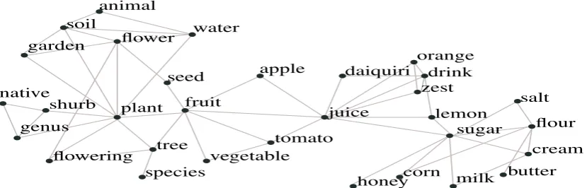
A simple way to bootstrap the manifold recreation process is to build a domain around each word, i.e., the semantic neighborhood of each word defines a domain. For example, in Figure 1 we show the semantic neighborhood offruit. The connections between words indicate high semantic similarity, i.e., this is a pruned semantic similarity graph of all words in the semantic neighborhood of the word ‘fruit’. It is clear from this example that in a typical neighborhood there exist word pairs that should be
[image:3.595.91.506.303.436.2]native genus b shurb b plant flowering b tree b species b b garden b soil b animalb water b seed flower b b fruit b vegetable b apple juice daiquiri b orange b drink b zest b lemon sugar salt b flour b cream b butter b b b milk b corn b honey b tomato b b b b
Figure 1: Visualization of the semantic neighborhood of the word ‘fruit’.
‘connected’ to each other because they have close semantic relation, like{flower,plant}and others that should not be ‘connected’ because they are semantically apart, like{garden,salt}. Asparse encodingof the semantic similarity relations in a neighborhood is needed in order to achieve (via multi-dimensional scaling) a parsimonious representation with good geometric properties1.
The graph connectivity or sparseness matrix identifies the word pairs that should be encoded in a neighborhood is defined as ˜S ∈ {0,1}n×n, where value ˜S(i, j) = 1indicates that the ith, jth word
pair is encoded, while ˜S(i, j) = 0 indicates that the pair is ignored (n is the number of words and
i, j= 1, .., nin the neighborhood). We define the degree of sparseness of matrix˜Sas the percentage of
0’s in the matrix.
4 Dimensionality Reduction
In this section, the Sparse Projection (SP) algorithm is described (see also Algorithm 1). SP is the core algorithm for constructing manifold DSMs presented in Section 5. SP is a dimensionality reduction algorithm that projects a set ofnwords into a vector space ofddimensions. The input to the algorithm is a dissimilarity or semantic distance matrix P ∈ Rn×n, where elementP(i, j) encodes the degree
of dissimilarity between wordswi andwj. The output of SP are thed-dimensional coordinate vectors
of then projected words that form a matrixX ∈ Rn×d. Each row xi ∈ R1×dof matrix X ∈ Rn×d
corresponds to the coordinates of the ith word wi. Once X is estimated the dissimilarity matrix is
recomputed and updated to new values, as discussed next. Each paragraph that follows corresponds to a module in Algorithm 1.
1Compare for example with Isomap (Tenenbaum et al., 2000) were a short- and long-distance metric is used. When using
Semantic Distance Re-estimation: Given the matrixX ∈ Rn×d containing the vector projections of
words in thed-dimensional space, the dissimilarity matrix is re-estimated using the Euclidean distance2.
LetPˆ ∈Rn×nbe the matrix with the new dissimilarity scores then the new dissimilarity score between
wordswiandwj is simply:Pˆ(i, j) = kxi−xjk2, wherexi,xj are the vectors corresponding to words wi,wjrespectively,i, j= 1, .., nandk.k2is the Euclidean norm.
Connectivity Graph and Sparsity: As discussed in Section 3, given a set of words only a small
subset of lexical relations should be explicitly encoded between pairs of these words. Therefore, the SP algorithm should only take into account strongly related word pairs and ignore the rest. This is the main difference between our approach compared to the generic MDS algorithm proposed in (Torgerson, 1952). In order to apply the sparseness constraint, we first construct the connectivity matrix˜S∈ {0,1}n×n. Word pairs(w
i, wj)with small similarity values (or equivalently large semantic
distance) are penalized: zero values are assigned to their corresponding position(i, j)in ˜Smatrix. In essence, the matrix ˜Sis obtained by hard{0,1}thresholding on the dissimilarity matrixP: all values that are under a threshold are set to 0, while all values equal or greater to the threshold are set to 1. Letnbe the number of words under investigation, then the number of word pairs is p = n·(n2−1). The degree of sparseness is defined as the number of unordered word pairs(wi, wj),i6=jwhere˜S(i, j) = 0
normalized over the total number of pairsp3.
Error Criterion: The algorithm employs a local and a global error criterion defined as follows:
1. The local error corresponds to the projection error for each individual wordwi e ∈ Rn×1, where i = 1...n and is defined as the sum of the dissimilarity matrix errors before and after projection computed only for the words that are ‘connected’ towi, as follows:
ei= n
X
j=1
˜S(i, j)·Pˆ(i, j)−P(i, j)2 (1)
2. The global error of the projection is simply the sum over local errors for all words:etot =Pni=1ei
Algorithm 1Sparse projection (SP)
Require: v// Vocabulary: vector ofnwords
Require: P//n×ndissimilarity matrix
1: ˜S←ComputeConnectivityMatrix(S) 2: foreach wordwi∈vdo
3: Xi ←RandomInitialization(Xi)
4: end for
5: k= 0// Iteration counter: initialization
6: ektot = inf// Global error: initialization
7: repeat
8: k=k+ 1
9: foreach wordwi ∈vdo
10: foreach directionzdo
11: X←MoveWordToDirection(wi, z)
12: ezi ←ComputeLocalError(˜S,P,X,i)
13: end for
14: zˆi ←FindDirectionOfMinLocalError(ezi)
15: X= MoveWordToDirection(wi,ziˆ)
16: end for
17: ektot←UpdateGlobalError(˜S,P,X)
18: untilektot−1 < ek
tot// Stopping condition 19: Pˆ ←SemanticDistanceReestimation(X) 20: P˜ ←SparseDistanceNormalizedRanges(Pˆ,˜S)
21: return X//n×dmatrix with coordinates;
22: return ˜S//n×nmatrix with connections;
23: return Pˆ //n×nupdated dissimilarity matrix;
24: return P˜ //n×nsparse-normalized distances;
Random Walk SP: In function MoveWordToDirection(·) of Algorithm 1, the pseudo-variabledirection
zrefers to a standard set of perturbations of each word in thed-dimensional space. For example, if the dimension of the projection isd= 2then the coordinates of each word are modeled as(k1, k2), where
k1, k2 ∈ R. A potential set of perturbations are the following: (k1, k2 +s),(k1, k2−s),(k1+s, k2) and(k1 −s, k2), wheresis the perturbation step parameter of the algorithm. For coordinates systems normalized in[0,1]dwe chose a value ofsequal to0.1. Good convergence properties to global maxima
have been experimentally shown for this algorithm for multiple runs on (noisy) randomly generated data. 2Other metrics, e.g., cosine similarity, have also been tested out but results are not shown here due to lack of space. Euclidean
distance performed somewhat better that cosine similarity for the semantic similarity estimation task.
Sparse Semantic Distance Normalized Ranges: This function normalizes all the distance scores ofPˆ
in a range of values, [0 r1], wherer1 ∈ R+ is an arbitrary positive constant and also it imposes the sparsity constraint as follows: if˜S(i, j) = 0thenP˜(i, j) =r1. If ˜S(i, j) = 1thenP˜(i, j) =r2·Pˆ(r3i,j), wherer3is the maximum distance over all ‘connected’ pairs, i.e. r3 ,max{Pˆ ˜S}, withdenoting the Hadamard product, andr2∈R+can be either equal tor1or slightly smaller thanr1. The assignment ofr2 < r1 aims to differentiate the ‘unconnected’ pairs from the ‘connected’ but dissimilar ones4.
5 Low-Dimensional Manifold DSMs
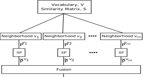
The end-to-end low-dimensional manifold DSM (LDMS) system is depicted in Figure 2. Note that v1,v2, ...,v|V| ∈V are the domains or sub-manifolds of the LDMS, for each domainvia separate DSM
[image:5.595.160.439.227.377.2]is built. V is the set of domains (concept vocabulary) and|V|denotes to the cardinality of V. The input
Figure 2: LDMS system.
to LDMS is a (global) similarity matrix S ∈ Rn×n, wheren is the total number of tokens (words) in
the LDMS model. Note thatScan be estimated using any of the baseline semantic similarity metrics5
presented in Section 2. Since the SP algorithm uses as input a dissimilarity or semantic distance matrix, the pairwise word similarity matrixS ∈ Rn×n is transformed to a semantic distance (or dissimilarity)
matrixP ∈Rn×nas: P(i, j) =c
1·e−c2·S(i,j) wherec1, c2 ∈Rare constants and the i,jindexes run from1ton. In this work, we usedc1=c2=20. The transformation defined by (5) was selected in order to non-linearly scale and increase the relative distance of dissimilar words compared to similar ones6.
The steps followed by the LDMS system are the following:
1. Domain Selection: The domains v1,v2, ...,v|V| are created as follows: for each word wi in our
model we create a corresponding domain vi that consists of all the words that are semantically
similar towi, i.e., the ith domain is the semantic neighborhood of word wi. Thus in our model the vocabulary size is equal to the domain set cardinality, i.e.,n = |V|. Domain vi is created by
selecting the topN most semantically similar words towi based on the (global) similarity matrix
S ∈ Rn×n. We have experimented with various domain sizes N ranging between 20 and 200
neighbors; note that each word in the LDMS may belong to multiple domains.
2. Sparse Projections on Domains: Following the selection of domain vi ∈V the (local) dissimilarity
matrix for each domain Pvi ∈ RN×N is defined as a submatrix of P ∈ Rn×n. Then, the SP algorithm is applied to each domain separately, resulting in i = 1, ..,|V| re-estimated bounded semantic distance matricesP˜vi.
3. Fusion: To reach a decision on the strength of the semantic relation between wordswiandwj the
semantic distance matrices from each domain P˜vi must be combined. Only domains were both wordswi andwj appear are relevant in this fusion process. This procedure is described next. 4We experimented with various values forr
1andr2achieving comparable performance; we selectedr2 ≈0.9r1that had slightly better performance. The value ofr1can be chosen arbitrary, the results reported here were obtained forr1 = 20and
r2= 18.
5.1 Fusion
Motivation: Given a set of wordsL={w1, w2, ...wn}we assume that their corresponding set of word
senses7isM ={s11, s12, .., s1n1, .., .., sn1, sn2, .., snn
n}. The set of senses is defined asM =∪ni=1Mi,
whereMi={si1, si2, ..., sini}is the set of senses for wordwi. LetS(.)be a metric of semantic similar-ity, e.g., the metric defined in Section 2, which is symmetric, i.e.,S(x, y)≡S(y, x). The notationsSw(.)
andSs(.)are used in order to distinguish the similarity at word and sense level, respectively. According to
the maximum sense similarity assumption (Resnik, 1995), the similarity betweenwiandwj,Sw(wi, wj), is defined as the pairwise maximum similarity between their corresponding sensesSs(sik, sjl):
Sw(wi, wj)≡Ss(sik, sjl), where (k, l) = argmax
(p∈Mi,r∈Mj)
Ss(sip, sjr).
Note that the maximum pairwise similarity metric (or equivalently the minimum pairwise distance metric) is also known as the “common sense” set similarity (or distance) employed by human cognition when evaluating the similarity (or distance) between two sets.
Fusion of local dissimilarity scores: Next we describe a domain fusion model that follows the
min-imum pairwise distance (dissimilarity) principle motivated by human cognition. The steps for the re-computation of the (global) dissimilarity between words wiand wjare:
1. Search for all the domains where wi and wj co-exist.
2. LetU ⊂V be the subset of domains from the previous step. The distances between words wi and
wjare retrieved from domain dissimilarity matricesP˜ufor allu∈U. The distances are stored into
vectord∈R|U|×1.
3. Motivated by the maximum sense similarity assumption (see above) the dissimilarity between wi
and wj is defined as8:
ˆ
P(i, j) = min
k=1..|U|{dk} (2)
4. If words wi and wj do not co-exist in any domain then r1 is assigned as their dissimilarity score, wherer1is the upper bound ofP˜u matrices as defined in the previous section.
For example, let one pair of words(w1, w2)co-exists in|U|= 3different domains with corresponding local distancesd= [9 20 11]then the global distance of(w1, w2)is 9.
6 Evaluation
In this section, we evaluate the performance of the proposed approach with respect to the task of simi-larity judgment between nouns. Results are reported with respect to several domain/neighborhood sizes, sparse percentages and domain dimensions.
The performance of similarity metrics were evaluated against human ratings from three standard datasets of noun pairs, namely WS353 (Finkelstein et al., 2001), RG (Rubenstein and Goodenough, 1965)MC(Miller and Charles, 1991). The first and the second datasets consist of the subset of 272 and 57 pairs, respectively, that are also included in SemCor39corpus, while the third dataset consists of 28
noun pairs. The Pearson’s correlation coefficient was selected as evaluation metric to compare estimated similarities against the ground truth.
The similarity matrix computed using the Google-based Semantic Relatedness (Gracia et al., 2006) was used as baseline, as well as to bootstrap the LDMS global similarity matrixS, for a list of 8752 nouns extracted from the SemCor3 corpus10. The performance of the proposed LDMS approach is presented
in Table 1. In addition, the performance of other unsupervised similarity estimation algorithms are reported for comparison purposes: 1) SEMNET is an alternative implementation of unstructured DSMs based on the idea of semantic neighborhoods and networks (Iosif and Potamianos, 2013) 2) WikiRelate! includes various taxonomy-based metrics that are typically applied to the WordNet hierarchy; the basic 7This is a simplification. In reality, some of the word senses will be the same, so strictly speaking this is not a set definition. 8Other fusion methods have also been evaluated, e.g., (weighted) average. Results are omitted here due to lack of space.
Minimum pairwise distance fusion outperformed other fusion schemes.
9http://www.cse.unt.edu/˜rada/downloads.html 10The baseline similarity matrix and the 8752 nouns are public available in:
idea behind WikiRelate! is to adapt these metrics to a hierarchy extracted from the links between the pages of the English Wikipedia (Strube and Ponzetto, 2006) . 3) TypeDM is a structured DSM (Baroni and Lenci, 2010), 4) AAHKPS1 constitutes an unstructured paradigm of DSM development using four billion web documents that were acquired via crawling (Agirre et al., 2009), 5) Moreover, two well-established dimensionality reduction algorithms (Isomap and LLE) that support the manifold hypothesis, were applied to the task of semantic similarity computation11. LDMS, Isomap and LLE were given as
input the matrixP∈ Rn×n, wheren = 8752is the number of words in our models. Isomap and LLE
used dimensionality reduction down tod= 5and neighborhood size equal toN = 120. SEMNET was run for neighborhood size equal toN = 100. While LDMS run for dimensionality down to d = 5,
domain/neighborhood size equal to N = 140 and degree of sparseness 90%. The proposed LDMS
system surpassed the performance of the baseline system for all three datasets, as well as the performance of the other corpus-based approaches for the WS353 and MC datasets. The dimensionality reduction algorithms (Isomap - LLE) are shown to perform poorly for this particular task.
Datasets Algorithm
Baseline SEMNET WikiRelate! TypeDM AAHKPS1 Isomap LLE LDMS
WS353 0.61 0.64 0.48 - - 0.14 0.04 0.69
RG 0.81 0.87 0.53 0.82 - 0.04 0 0.86
MC 0.85 0.91 0.45 - 0.89 -0.04 -0.04 0.94
Table 1: Performance of various algorithms for the task of similarity judgment.
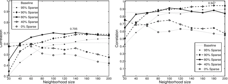
The performance (Pearson correlation) of the LDMS approach is shown in Figures 3a, 3b and 4a as a function of neighborhood size and degree of sparseness. Results are presented for all three datasets: WS353, MC, and RG. The baseline performance is also plotted (dotted line). For all three datasets, we see a clear relationship between neighborhood size, degree of sparseness and performance. Sparse representations achieve peak performance for larger neighborhood sizes. High degree of sparseness between 80 and 90% achieves the best results for domain/neighborhood sizes between 100 and 140. The figures show that there is potential for even better performance by fine-tuning the LDMS parameters.
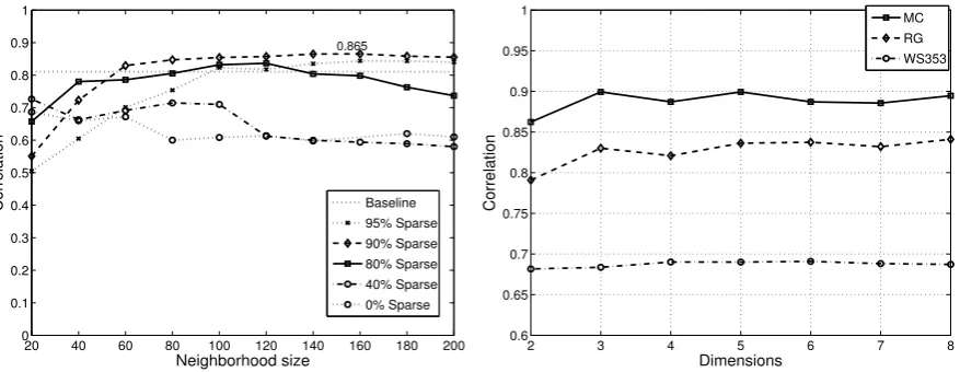
The performance of LDMS is shown in Figure 4b as a function of the projection dimensiond. The de-gree of sparseness is fixed at 80% and the domain/neighborhood size is equal to 100 for all experiments. It is observed that the performance for all three datasets remains relatively constant when at leastd= 3
is used. In fact results are slightly better for d = 3than for higher dimensions but the differences in performance are not significant. The results suggest that even a 3D sub-space is adequate for accurately representing the semantics of each underlying domain.
20 40 60 80 100 120 140 160 180 200 0.3
0.4 0.5 0.6 0.7 0.8 0.9 1
0.705
Neighborhood size
Correlation
Baseline
95% Sparse
90% Sparse 80% Sparse
40% Sparse
0% Sparse
20 40 60 80 100 120 140 160 180 200 0
0.1 0.2 0.3 0.4 0.5 0.6 0.7 0.8 0.9 1
0.947
Neighborhood size
Correlation Baseline
95% Sparse 90% Sparse
80% Sparse
40% Sparse
[image:7.595.79.519.542.705.2]0% Sparse
Figure 3: Performance as a function of domain size N and sparseness percentage for the (a) WS353 dataset and (b) MC dataset.
11LDMS is not directly comparable with Isomap-LLE algorithms because it represents only the domains in low-dimensional
20 40 60 80 100 120 140 160 180 200 0
0.1 0.2 0.3 0.4 0.5 0.6 0.7 0.8 0.9 1
0.865
Neighborhood size
Correlation Baseline
95% Sparse
90% Sparse
80% Sparse
40% Sparse
0% Sparse
2 3 4 5 6 7 8
0.6 0.65 0.7 0.75 0.8 0.85 0.9 0.95 1
Dimensions
Correlation
[image:8.595.83.522.63.233.2]MC RG WS353
Figure 4: Performance for the (a) RG dataset as a function of domain sizeN and sparseness percentage and (b) WS353, MC, RG datasets as a function of projection dimensiond.
7 Conclusions
In this work, we proposed a novel, hierarchical DSM that was applied to semantic relation estimation task obtaining very good results. The proposed representation consists of low-dimensional manifolds that are derived from sparse projections of semantic neighborhoods. The core idea of low dimensional subspaces was motivated by cognitive models of conceptual spaces. The validity of this motivation was experimentally verified via the estimation of semantic similarity between nouns. The proposed approach was found to be (at least) competitive with other state-of-the-art DSM approaches that adopt flat feature representations and do not explicitly include the sparsity and dimensionality as a key design parameter.
The poor performance of Isomap and LLE can be attributed to the nature of the specific application, i.e., word semantics. A key characteristic of this application is the ambiguity of word senses. These algorithms assume only one sense for each word (i.e., a word is represented as a single point in a high-dimensional space). Although the disambiguation task is not explicitly addressed, LDMS approach handles the ambiguity of words by isolating each word’s senses in different domains.
Our initial intuition regarding the semantic fragmentation of lexical neighborhoods due to singularities introduced by word senses was supported by the high performance when large (i.e., 80% - 90%) degree of sparseness was imposed. The hypothesis of low-dimensional representation was validated by the finding that as little as three dimensions are adequate for representing domain/neighborhood semantics. It was also observed that the parameters of the LDMS model, i.e., number of dimensions, neighborhoodsize and degree of sparseness, are interrelated: very sparse projections achieve best results with very low dimensionality when large neighborhood sizes are used.
This is only a first step toward using ensembles of low-dimensional DSMs for semantic relation esti-mation. As future work we plan to further investigate the creation of domains based on more complex geometric properties of the underlying space (Kreyszig, 2007). A more formal investigation of the re-lation between sparseness, dimensionality and performance is also needed. Finally, creating multi-level hierarchical representations that are consistent with cognitive organization is an important challenge that can further improve manifold DSM performance.
Acknowledgments
References
E. Agirre, E. Alfonseca, K. Hall, J. Kravalova, M. Pas¸ca, and A. Soroa. 2009. A study on similarity and relatedness using distributional and wordnet-based approaches. InProceedings of Human Language Technologies, pages 19–27. Association for Computational Linguistics.
R. G Baraniuk and M. B Wakin. 2009. Random projections of smooth manifolds. Foundations of computational mathematics, 9(1):51–77.
M. Baroni and A. Lenci. 2010. Distributional memory: A general framework for corpus-based semantics. Com-putational Linguistics, 36(4):673–721.
Y. Bengio, A. Courville, and P. Vincent. 2013. Representation learning: A review and new perspectives.
D. Bollegala, Y. Matsuo, and M. Ishizuka. 2007. Measuring semantic similarity between words using web search engines. InProc. of International Conference on World Wide Web, pages 757–766, Banff, Alberta, Canada. Ingwer Borg. 2005. Modern multidimensional scaling: Theory and applications. Springer.
A. Budanitsky and G. Hirst. 2001. Semantic distance in wordnet: An experimental, application-oriented evalua-tion of five measures. InWorkshop on WordNet and Other Lexical Resources.
O. Corby, R. Dieng-Kuntz, F. Gandon, and C. Faron-Zucker. 2006. Searching the semantic web: Approximate query processing based on ontologies. Intelligent Systems, IEEE, 21(1):20–27.
D. L Donoho and C. Grimes. 2003. Hessian eigenmaps: Locally linear embedding techniques for high-dimensional data. Proceedings of the National Academy of Sciences, 100(10):5591–5596.
L. Finkelstein, E. Gabrilovich, Y. Matias, E. Rivlin, Z. Solan, G. Wolfman, and E. Ruppin. 2001. Placing search in context: The concept revisited. InProceedings of the 10th international conference on World Wide Web, pages 406–414. ACM.
P. Gardenfors. 2000. Conceptual spaces: The geometry of thought. Cambridge, Massachusetts: USA. ISBN, 262071991.
J. Gracia, R. Trillo, M. Espinoza, and E. Mena. 2006. Querying the web: A multiontology disambiguation method. InProc. of International Conference on Web Engineering, pages 241–248, Palo Alto, California, USA. G. Grefenstette. 1994. Explorations in Automatic Thesaurus Discovery. Kluwer Academic Publishers, Norwell,
MA, USA.
Z. Harris. 1954. Distributional structure.Word, 10(23):146–162.
E. Iosif and A. Potamianos. 2010. Unsupervised semantic similarity computation between terms using web documents. Knowledge and Data Engineering, IEEE Transactions on, 22(11):1637–1647.
E. Iosif and A. Potamianos. 2013. Similarity computation using semantic networks created from web-harvested data. Natural Language Engineering (DOI: 10.1017/S1351324913000144).
I. Jolliffe. 2005. Principal component analysis. Wiley Online Library.
J. Karlgren, A. Holst, and M. Sahlgren. 2008. Filaments of meaning in word space. InAdvances in Information Retrieval, pages 531–538. Springer.
E. Kreyszig. 2007.Introductory functional analysis with applications. Wiley. com.
P. Li, T. J Hastie, and K. W Church. 2006. Very sparse random projections. InProceedings of the 12th ACM SIGKDD international conference on Knowledge discovery and data mining, pages 287–296. ACM.
N. Malandrakis, A. Potamianos, E. Iosif, and S. S Narayanan. 2011. Kernel models for affective lexicon creation. InINTERSPEECH, pages 2977–2980.
G. A Miller and W. G Charles. 1991. Contextual correlates of semantic similarity. Language and cognitive processes, 6(1):1–28.
P. Resnik. 2011. Semantic similarity in a taxonomy: An information-based measure and its application to prob-lems of ambiguity in natural language. arXiv preprint arXiv:1105.5444.
S. T Roweis and L. K Saul. 2000. Nonlinear dimensionality reduction by locally linear embedding. Science, 290(5500):2323–2326.
H. Rubenstein and J. B Goodenough. 1965. Contextual correlates of synonymy. Communications of the ACM, 8(10):627–633.
Michael Strube and Simone Paolo Ponzetto. 2006. Wikirelate! computing semantic relatedness using wikipedia. InAAAI, pages 1419–1424.
J. B Tenenbaum, V. De Silva, and J. C Langford. 2000. A global geometric framework for nonlinear dimensional-ity reduction.Science, 290(5500):2319–2323.
J. B Tenenbaum, C. Kemp, T. L Griffiths, and N. D Goodman. 2011. How to grow a mind: Statistics, structure, and abstraction.science, 331(6022):1279–1285.
Warren S Torgerson. 1952. Multidimensional scaling: I. theory and method.Psychometrika, 17(4):401–419. S. Tsuge, M. Shishibori, S. Kuroiwa, and K. Kita. 2001. Dimensionality reduction using non-negative matrix
factorization for information retrieval. InSystems, Man, and Cybernetics, 2001 IEEE International Conference on, volume 2, pages 960–965 vol.2.
J. V´eronis. 2004. Hyperlex: Lexical cartography for information retrieval. Computer Speech and Language, 18(3):223–252.
Jianzhong Wang. 2011. Maximum variance unfolding. InGeometric Structure of High-Dimensional Data and Dimensionality Reduction, pages 181–202. Springer.
J. Weston, F. Ratle, H. Mobahi, and R. Collobert. 2012. Deep learning via semi-supervised embedding. InNeural Networks: Tricks of the Trade, pages 639–655. Springer.