Robust Parsing Using a Hidden Markov Model

(1)

I

n

t

mm

nm

n

I

n

nm

mm

I I

I

mm

l

mm

U

Robust Parsing Using a Hidden Markov Model

Wide R. H o g e n h o u t Yuji M a t s u m o t o Nara Institute of Science and Technology

A b s t r a c t . Recent approaches to statistical parsing include those that estimate an approximation of a stochastic, lexicalised gr~mm~x directly from a treebank and others that rebuild trees with a number of trse-coustructing operators, which are applied in order according

to a stochastic model when parsing a sentence. In this paper we take an ehtirely di~erent approach to statistical parsing, as we propose a method for parsing using a Hidden Markov Model. W e describe the stochastic model and the tree construction procedure, and we report results on the Wall Street Journal Corpus.

1 Introduction

Recent approaches to statistical parsing include those that estimate an approximation of a

stochastic, lexicalized ~rammar directly from a treebank (Colll-.q~ 1997; Charuiak, 1997) and others that rebuild trees with a number of tree-construction operators, which are applied in order according to a stochastic model when parsing a sentence (Magerman, I995; Ratna- parldd, 1997). The results have been around 86% in labeled precision and recall on the Wall Street Journal treebank (Marcus, Santorini, and Marcinldewicz, 1994).

In this paper we take an entirely different approach to statistical parsing. We propose a method for left to fight parsing using a Hidden Markov Model (HMM). The results we obtain are not as good as the more general approaches mentioned above, which consider the whole sentence rather then working in an incremental fashion, but the method does give a number of interesting new perspectives. In particular, it can be applied in an environment that requires left to right processing, such as a speech recognition system, it can easily process text that has not been separated into sentences (for example when punctuation is mi~ing or when~processing ungrammatical, spoken text), and it can give a shallow parse (i.e., leaving out long distance dependencies) as it is focused On local context. It also makes the parsing process closer to the way humans process language, although we do not explore this psychological aspect in this paper.

In the next three sections we will discuss the way we decide the syntactic context of a word (%raversal strings"), how this can be used for parsing and how a tree can be constructed ~om them. The following four sections discuss the HMM model used to predict a syntactic context for every word. The last two sections discuss the results, conclusions and future perspectives.

2 Traversal Strings

Take the sentence "I a m singing in the rain." This can be analyzed as indicated in figure I, where the first line of symbols above the text indicates parts of speech as used in the Wall Street Journal Corpus (for example, V B G stands for "verb -gerund or present participle"). The abbreviations used for nonterminals are self-explanatory.

(2)

m

ss

$

PP VBP VBG IN DT NN I a m .~in~n~ in the rain

F i g u r e 1. Example of Syntactic Analysis.

We will call these strings (excluding the word and its tag) traversal strings. It will be obvious that this representation is very redundant, and it is exactly this property that we will exploit. But first we note it is also possible to carry out the inverse action of reconstructing the tree from a set of traversal strings. Later we will describe a robust, heuristic algorithm for reconstructing the tree.

The basic concept of parsing with traver°~l strings is t h a t after seeing a word, one considers a number of possible tree contexts in which t h a t word normally occurs. The most likely ones are selected b o t h b y considering the likelihood of a context occun'ing with a word and the likelihood of a context following another context. As for the last relation, it is here that the redundance becomes me~nlngful; since neighboring traversal strings are often partially or completely equal.

Oflazer (1996) used a similar structure called "vertex lists" which he defined as the path from a leaf to the root of the tree but, different from our definition, including the tag and the word. Oflazer uses vertex lists for error-tolerant tree-matching. In some cases trees can be said to match approximately, and using vertex lists to quantify the amount of difference between trees, Oflazer shows how trees similar to a given tree can be retrieved from a database (treebank). As will be clear from what follows, we use traversal strings in a completely different way, and to the best of our knowledge these strings have not been used for parsing before.

The work of Jcehi and Srinivas (1994) actually comes closer to our work. While we attach traversed strings to word-tag pairs, they do the same with elementary structures in a Lexi- calized Tree-Adjolnlng Grammar, called Supertags. This is a partial tree t h a t only contains one lexical word, as well as part of its context. Joshi and Srinlvas show how, by statisti- cally choosing such structures for each word in a sentence, t h e y are able to disambiguate syntactical structure. Note however t h a t the results they give are not comparable to ours as they only tested on short sentences, and report on the accuracy of Supertags rather than bracket-accuracy or recall.

I/PP -> NP -> S

am/VBP -> VP -> VP -> S singing/VBG -> VP -> VP -> S i n / I N -> PP -> VP -> S

the/DT -> NP -> PP -> VP -> S rain/NN -> NP -> PP -> VP -> S

. / . - > S

(3)

m

3 Parsing with Traversal Strings

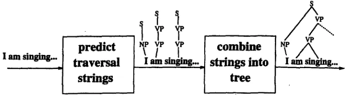
Figure 2 shows the system design. When presented with a sentence, the first component finds the most likely set of part of speech tags (not shown) and traversal strings matching the words in the sentence. After this a second component assembles a tree from the traversal strings.

l

predict

s p /P ~

[ combine

l am singing.., traversal

Iamsm.~...J

strings into 1..

Iamsmghlg...

-[ strings

1

tree

!

F i g u r e 2. System Design

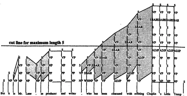
The prediction of traversal strings presents us with a problem, since traversal strings of arbitrary length are too numerous to be predicted accurately. To see our answer to this problem it is instructive to look at the analysis of a longer sentence, please see figure 3. In particular, notice the shaded areas that show how traversal strings of neighboring words are often equal or partially equal. The most common relation that is seen is a 'shift', where the vertex at position n for word wi becomes vertex n + 1 for word wi+l. At the bottom of the traversal string one vertex is added, and nothing else changes.

This illustrates the next step we will take. Even after cutting off traversal strings at a fixed maximum length, it is still possible to reconstruct the tree. The dotted line in figure 3 shows how traversal strings are cut off at a maximum length of 5 vertices. Having part of the traversal string still leaves it possible to see that a particular word is likely to be in the same context as his neighbor. More generally, we look at what subtrees are likely to share part of their context with other, neighboring subtrees. We will show how doing this iteratively makes it possible to restore the tree with a high degree of accuracy.

4 Transforming Traversal Strings into Trees

We use a heuristic algorithm for reconstructing a tree from traversal strings. This includes '~artial" traversal strings, but we simply refer to them as traversal strings since we will always be working with partial traversal strings anyway. This is a brief, informal description of the algorithm. A complete technical description is given in (Hogenhout, 1998).

The algorithm is based on the heuristic that best matches should go first. The best match is decided by checking neighboring strings (or, later, subtrees) for equal nonterminals starting at the top of either side. The pair with the most matching nonterminals is merged as displayed in figure 4. This process is repeated until one tree remains, or when there are no more matching neighbors.

For example, the choice

[image:3.612.124.484.219.328.2]

(4)

F i g u r e 3. Similarity between Traversal Strings and cut at maximum length 5

Wi W2 W3 W4 W5 W6 W7 Ws W9 Wlo

F i g u r e 4. "[~raversal Strings merged into (sub)trees

would initially be decided in favor of the and

rain,

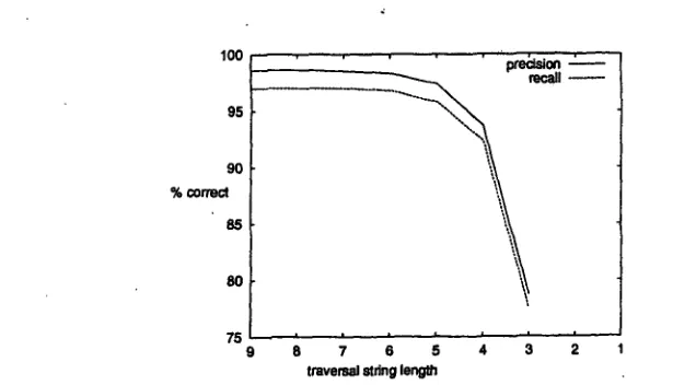
and.after they are merged completely, the top three nonterminals would be merged to those of i~

There is an easy way of testing this algorithm. One can take trees from a treebank, convert the trees to traversal strings, then use the algorithm to reconstruct the trees. Figure 5 shows the labeled accuracy and recall of these reconstructed trees when compared to the original treebank trees, for various maximum traversal string lengths.

The accuracy is calculated as

number of identical brackets with identical nonterminal

accuracy -- number of brackets in system parse (1)

and the recall as

number of identical brackets with identical nonterminal

[image:4.612.134.493.103.288.2]

(5)

Even for long traversal strings the original tree is not reconstructed completely. This happens, for example, when two identical nonterminals are siblings, as in the sentence "She ga~e [NP

the man] [NP a book]."

It is of course possible to solve such problems with a post-processor t h a t tries to recognize such situations and correct them whenever they arise. But as can be seen it only involves a small percentage (about 2%) of all brackets and for this reason it is not very significant at this stage.

lOO 95 9 0 % correct

85 80 75

recall ~

i | i ~, J . . . .

8 7 6 5 4 3 2

travemal stdng length

F i g u r e 5. Upper Bound Imposed by Tree Construction Algorithm

The graph shows t h a t if we are capable of predicting up to 5 or more vertices, the algorithm will be able to do very well. If we can only predict up to 4 vertices we still have a high upper bound, but it is slightly lower~ Predicting up to 3 or less vertices however will not produce useful results.

It must however be stressed t h a t this .is only an upper bound and does not reflect the performance of a useful system in any way. The upper bound only helps to pin down the border line of 4-5 vertices, and what really counts in practice is how the algorithm will do when the traversal strings that are predicted contain errors--as they undoubtedly will.

5 Guessing Traversal Strings

We will now look at the question of how to predict traversal strings. As will become clear w h e n inspecting the equation this bears similarity to part-of-speech tagging. But there is one factor that makes a big difference: we do not test on the correct traversal string, but on the result of the tree t h a t is reconstructed at the end. In many cases the traversal string t h a t is guessed is not correct, but similar to the correct traversal string, and a Similar traversal string will render much better results at tree reconstruction t h a n a completely different one. As usual our approach is maximizing the likelihood of the training dal~a. We will use a Hidden Markov Model which has traversal string-tag combinations as states and which produces words as output. We do not re~stimate probabilities using the Bantu-Welch algorithm (Bantu,

1972) but we use smoothed Maximum Likelihood estimates from treebank data.

[image:5.612.120.438.195.371.2]

(6)

II

We take the probability of a sentence to be

p(Wl--.~.Ort) =

~'p(wl...w~lT,,q)

(3)

7",8

~ ~pC~, Is,, t,)p(~,+,.,

t,+~

I,~.

t,),

(4)

7",8 in0

corresponding to the transition and output probabilities of a hidden markov model. In practice the probabilities p(wi[si, ti) and p(s~+l,

ti+l]s,,

t,) can not be estimated directly using Maximum Likelihood because of sparse data. For this reason we smooth the estimates with our version of lower-order models as follows:

~(w~lsl, ti) = A,it~p(wils,, ti) +

(1 - ;~,m)p(w, lt0 (5) where the interpolation factor •sit, is a d j u s t e d for different values of si and t, as suggested in (Bahl, Jelinek, and Mercer, 1983). We also divide the

si-ti pa~r values over different buckets

so that all pairs in the same bucket have the same ,~ parameter. It should be noted that we have a special word which stands for "nnlcnown word," to take care of words that were not seen in the training data.

We do something similar for p(si+l,

ti+llsi, tO,

namely

~(s~+lt,+lls. tO = 6~,pCs~+~t~+iIs. td

+ 6~mpCsi+lt~+lltd

+

6~mpCs,+lt,+l)

(fi) where of course 6~,ti + ~it, + 6~ti = 1. The interpolation factors axe bucketed in the same w~y.

Using the obtained model we choose T and ,q by maximizing the probability of the sentence that w e wish to analyse:

(~r, s)" =

arsma~p((7", S)lw2...w.)

(7)

(r,s)

n

argmax ITp(w~ls~,

tdp(si+2, ti+l Is.

to

(8)

¢r,s) ~ o

which can be resolved using the Viterbi-algorithm (Viterbi, 1967).

6

S e l e c t i o n o f P a r t o f S p e e c h T a g s

The process outlined above still has one problem that will be central in the rest of the discussion. The number of traversal strings is easily a few thousand, and the number of part of speech tag-traversal string pairs is even larger. Clearly, the computational complexity of the algorithm is in calculating (8). But, given a word and the history up to that word, most tags and traversal strings can be ruled out immediately. We will therefore only consider a fraction of the possible part of speech tags and traversal strings. This section will discuss how we select part of speech tags.

The equation we use for selecting a tag is similar to the standard tagging HMM based model. We pretend for the time being that we are dealing with another stochastic process, namely one that only generates tags. We assume that

p(wl...w~) = y~p(wl...w~, 7")

(9)

T

n

~. ~_~ l'Ip(w~lti)p(ti+llti)

(10)

T i=O

(7)

m

[]

mm

m

n

m

mm

m

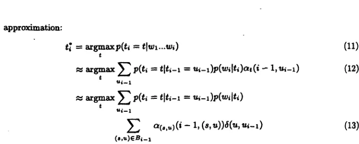
approximation:

1;~' = argm.axp(t:i = t:['wl...'w.i) (11)

t

= argmax ~ p(t, = tit,-1 = ~-l)p(w, lt,)atC/- I, ~-1)

(12)

t

= argmax ~ p(t, = tlt,-~ = ~-~)p(w, lt,)

t

U i - - 1

O~C.,,,)4i - 1, (s,u))6(u, u a - l ) (13) O,,'.,.)(E .ei- 1

where s is a traversal string, the symbol B i - I indicates the set of tag-traversal string pairs that is being considered for word wi-l, and ~ indicates the "forward probability" according to the

HMM.

As usual 64u, u~-l) -- 1 i f u = u~_~ and 0 otherwise. We will discuss later how the set B~-I is chosen, but this of course depends on the tags selected for the word wi-1. We distinguish between ~, (tagging model) and ~(~,~) (traversal string model).

We take two significant assumptions at this point. First, we do not really use the HMM indicated in 410), but in equation (12) we restrict ourselves to the forward probability. The second assumption we take is (13), i.e., we estimate the probability of the previous tag by the tag-traversal string pairs that were selected for the previous word. Using this method we do not need to implement the markov model for tags, we only need the tables for

p(t, lti_l)

and p(wdti ).

As we already need the last one for the traversal string model, we only need the (small) table

p(ti[t~-l)

especially for tagging.

We must emphasize that the tagging described here is only a first estimate. We consider the most ~lcely one, two or three tags according to this model and discard the rest. Once they are selected, these probabilities are discarded and we return to the regular model. The next section will describe how the tags are selected in the next phase.

7

S e l e c t i o n o f T r a v e r s a l S t r i n g s : F i r s t P h a s e

The next problem is how to select a few traversal strings given a word and a few tags, one of which is likely to be correct. The model we use for this pre~selection is actually more simple; as we ignore the selected traversal strings for previous words. 1 From the corpus we directly estimate in Maximum Likelihood fashion

P4w,, si, ti) (14)

and select the most likely travexsal strings si from this table. If there are too few samples for a particular word wi, the list is completed with the more general distribution

P(s,,t,),

(15)

again maximizing over si. We will have to consider that we do not have a single tag but several options, but we will first pretend that we do have one single tag.

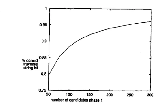
Figure 6 shows the results of this first phase, in case the maximum length of traversal strings is set to 5. If the best 50 candidates are selected according to 414), supplemented with selection according to (15) if necessary, we have the correct candidate between them about 80% of the time. That means that for 20% of the words, we can only hope that a similar traver-~al string will be available for them. If we use the best 300 candidates, we will miss the correct candidate for about one word per sentence. We must however emphas!ze two points: 1. The question is not only if we can select the correct candidate. It is crucial that, when

a wrong candidate is chosen, this is at least similar to the correct candidate.

[image:7.612.121.481.80.225.2]

(8)

0.95 0.9

% correct 0.85 traversal string hit

0.8

0 . 7 5 I I I i

5O IO0 150 2O0 25O 3O0

[image:8.612.172.435.95.271.2]

number of candidates phase 1

Figure 6. Hit percentage for first phase

Now we return to the tagging problem; after all we do not have the right tag available to us. We solve this, heuristically, as follows. Let a be the most likely tag, b the second most likely and c the third.

- If p(a)/p(b) > 50, select 300 candidates for tag a and ignore other tags.

- If 50 > p(a)/p(b) > 4 we select 300 candidates for tag a and more 100 candidates for tag b.

- If 4 >_ p(a)/p(b) we select 300 candidates for tag a, 200 candidates for tag b and 100 candidates for tag c.

This scheme gives more candidates for more ambiguous words, but as about 80% of all words fall in the first category and only 9% in the last category, this is not so bad. This list will contain the correct traversal string about 95% of the time.

8

S e l e c t i o n of Traversal S t r i n g s : S e c o n d P h a s e

The previous section explained how initial candidates can b e selected quickly from all possible sets. After these initial candidates were selected, the transition and output probabilities are calculated. Let again B~- 1 be the set of candidates considered for word w~_ 1. Then we need to calculate (regrouping the product as compared to (8)) the quantity

,~(8,t,) =

~

,~(8,t)p{,~,ls,,t,)p(8,,~,ls,0

(16)

(~,t)~Bi_1

where we set

1 if s0 = d u m m y and Co = d u m m y

(9)

- In the first phase we use equation (14) and select the best p candidates. (As explained, depending on tagging confidence we vary the number of candidates, so # should be thought of as an average.)

- In the second phase we use equation (16) and select the best 7 candidates.

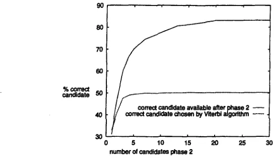
It will be clear t h a t we can choose 7 ( ( / z . We have illustrated this in figure 7, which displays the percentage of correct candidates for various values for 7, again using a maximum traversal string length.of 5. Note t h a t the computational complexity of the Viterbi algorithm will be

O(p~n)

where n is sentence length.

9O

8O

7O

6O

% correct candidate

50

40

30

f f . . . .

~ a t e

available after phase 2 - -

' correct candidate ¢ho6en by Viterbl algodthm

r i i i i

5

10

15

20

25

30

number of candidates

phase 2

F i g u r e 7. Hit percentage for second phase

Figure 7gives the percentage of cases in which the correct candidate is available (the upper line) and also the percentage of cases in which the correct candidate is chosen by the Viterbi algorithm. A remarkable fact arises from this figure: the percentage of traversal strings that are chosen correctly stabilizes at about 7 = 4. From t h a t point the percentage is about 50% and while increasing 7 increases the chance t h a t the correct one will be available, choosing it becomes more diiBcult and these two effects cancel each other out. Nevertheless the result continues to improve for higher 7, as better alternatives become available. We will put 7 to 15 as a higher number contributes little more to the final scores.

9 Parsing

We have now dealt with all parts of the parsing process. Whenever a new word is seen, a few tags are selected according to (13). After this a set of about 300 (depending on the confidence in the tags) traversal strings is selected according to (14) or (15). The forward probability of these candidates is calculated (16) and this is used to further reduce the candidates to 15 tag-traversal string pairs. This set is saved with their forward probabilities, and when the end-of-sentence signal is received the best series is given by the Viterbi algorithm. A tree is then produced according to the algorithm described in section 4.

[image:9.612.131.408.233.394.2]

(10)

go

85 oo

75 % corred

bracket 7O 65 60 3

] I

j /

4 5 6 7

mmdmmm ~nmm~ ~ ~

Figure 8. Precision and recall plotted again.qt maximum traversal string length

and section 23 (2,416 sentences) was used exclusively for testing. Figure 8 shows the labeled accuracy and recall for various maximum lengths that result from this data.

This shows that the optimal length is about 4, 5 or perhaps 6. This picture is slightly favoring the shorter lengths, since # and ~ are fixed while the longer lengths have more candidates to choose from. But on the other handl keeping p and ~7 fixed corresponds to giving the algorithm a certain time and letting it do its best in the given time• The longer lengths also have a disadvantage in that they lead to larger tables, using more memory.

The differences between 4, 5 and 6 axe minor, and the performance degrades seriously at 3 or 7. This shows that a maximum of 5 is a sensible choice. The first colnm, of table 2 gives detailed information about the final performance. It is also possible to restrict the parser to lower level structures, t~iclng only those parts which are the most safe, namely low-level brackets that do not depend on long distance dependencies. We carried this out by removing brackets covering more than three words and some particular nonterminals that often result in errors, such as SBAR~ These results axe indicated in the ~Shallow Parsing z c o l - r e ,

Table 2. Parsing Results

Measure Regular Score Shallow Parsing

labeled precision 75.6% 87.4%

labeled recall 72.9% 37.9%

unlabeled precision 79.5% 89.2%

unlabeled recall 76.6% 38.9%

crossing brackets per sentence 2.31 0.44

tagging accuracy 94.4%

speed on Spaxc Station 20 6.5 words/second

10

D i s c u s s i o n

[image:10.612.202.447.92.266.2] [image:10.612.183.434.517.623.2]

(11)

|

mm

U

[]

n

[]

m

U

m

U

m

[]

mm

m

performs quite reasonable and is very robust.

The score is less than the scores obtained by systems that consider the entire sentence with, in particular, the headwords of phrases. But the method creates new possibilities such as processing ungrammatical text and processing unpunctuated text. Shallow parsing is also a possible application.

As far as future directions are concerned, we would like to mention that our parsing strategy is not limited, to regular languages and HMM models. It is possible to switch to a history- based approach, where the choice of si depends on both the words wl...w~ and all earlier tags and traversal strings chosen by the system. In that case a statistical decision tree or a markov field can be used to model the optimal choice for s~ after seeing word

wi.

11 Acknowledgements

We would like to thank the anonymous reviewers for their useful comments.

References

Bald, Lalit R., Frederick Jelinek, and Robert L. Mercer. 1983. A maximum likelihood approach to continuous speech recognition.

IEEE Transactions on Pattern Analysis and

Machine Intelligence,

PAMI-5(2):l?9-190.

Baum, L.E. 1972. An inequality and associated maximization technique in statistical estimation for probabilistic functions of Markov processes.

Inequalities,

3:1-8.

Charuiak, E. 1997. Statistical parsing with a context-f~ee grammar and word statistics. In

Proceedings of the Fourteenth National Conference on Artificial Intelligence, AAAI,

pages 598-603.

Collins, M. J. 1997. Three generative, lexicalised models for statistical parsing. In Proceed-

ings of the 85th Annual Meeting of the Association for Computational Linguistics and 8th

Conference of the European Chapter of the Association for Computational Linguistics, pages

16-23.

Hogsnhout, Wide 1t. 1998.

Supervised Learning of Syntactic Structure.

Ph.D. thesis, Nara Institute of Science and Technology.

Joshi, Aravind K. and B. Srinivas. 1994. Disambiguation of super parts of speech (or supertags): Almost parsing. In

Proceedings of the 15th International Conference on Computa-

tional Linguistics (COLING-g4),

pages 154-160.

Magerman, D. M. 1995. Statistical declsion-tree models for parsing. In

Proceedings of the

33d Annual Meeting of the Association for Computational Linguistics,

pages 276-283. Marcus, Mitchell P., Beatrice Santorini, and Mary Ann Marcinkiewicz. 1994. Build- ing a large annotated corpus of English: the Penn Treebank.

Computational Linguistics,

19(2):313--330.

Oflazer, Kemal. 1996. Error-tolerant tree matching. In

Proceedings of the 16th International

Conference on Computational Linguistics (COLING-96),

pages 860--864.

Ratnaparkhi, Adwait. 1997. A linear observed time statistical parser based on maximum entropy models. In

Proceedings of the Second Conference on Empirical Methods in Natural

Language Processing.