Normalising Audio Transcriptions for Unwritten Languages

Proceedings of the 5th International Joint Conference on Natural Language Processing, pages 527–535, Chiang Mai, Thailand, November 8 – 13, 2011. c2011 AFNLP

Normalising Audio Transcriptions for Unwritten Languages

Adel Foda

_and

_{Steven Bird}

_{Department of Mathematics and Statistics}

†

_{Department of Computer Science and Software Engineering}

University of Melbourne, Victoria 3010, Australia

Abstract

The task of documenting the world’s lan-guages is a mainstream activity in linguis-tics which is yet to spill over into computa-tional linguistics. We propose a new task of transcription normalisation as an algo-rithmic method for speeding up the pro-cess of transcribing audio sources, leading to text collections of usable quality. We report on the application of sentence and word alignment algorithms to this task, before describing a new algorithm. All of the algorithms are evaluated over syn-thetic datasets. Although the results are nuanced, the transcription normalisation task is suggested as an NLP contribution to the grand challenge of documenting the world’s languages.

1

Introduction

The majority of the world’s 6800 languages are rel-atively unstudied. Although some of the world’s languages have been carefully described and anal-ysed, most of them have not yet even been docu-mented. Such documentation consists of ‘compre-hensive and transparent records supporting wide ranging scientific investigations of the language’ (Woodbury, 2010). In this context then, it is striking that 50 years of research in computational linguistics have so far only touched about 1% of the world’s languages. In 100 years, 90% will be extinct or on the way out (Krauss, 2007). Ac-cordingly, we set ourselves the following question: what can computational linguistics offer to support the urgent task of documenting and analyzing the world’s endangered languages? There have been other recent efforts to address this question, fo-cussing on interlinear text (Xia and Lewis, 2007; Baldridge and Palmer, 2009). Our focus is dif-ferent, being concerned with creating the unanno-tated text that is presupposed by this earlier work. We also differentiate our work from more general computational support for documentary and de-scriptive linguistics, such as tools for transcribing audio or editing lexicons.

Recently, Abney and Bird (2010) have proposed to incorporate machine translation (MT) into the workflow of language documentation. However, a significant challenge for this program is posed by the fact that the majority of the world’s languages are not written. How can NLP techniques be ap-plied to improve the speed and efficiency of audio transcription for unwritten languages?

The task of transcription differs from transliter-ation (Knight and Graehl, 1998) in several ways. Transliteration is required in the context of ma-chine translation for dealing with proper names, which are a common source of out-of-vocabulary items. The goal is to make the words pronounce-able in a target language having a different inven-tory of sounds and syllables, and having different grapheme-to-phoneme rules. Since the source and target languages have established orthographies, the correct placement of word boundaries is never in question.

Transcription, on the other hand, involves rep-resenting spoken utterances in written form. In the absence of a standard orthography or lexicon, two transcribers will usually represent sounds us-ing different symbols, and will often disagree on the placement of word boundaries. Transcribers may use a mixture of conventions from other lan-guages, e.g. ”vowels as in Italian, consonants as in English”, and may invent their own system of dia-critics. The goal is to faithfully capture all of the significant aspects of pronunciation. By obtain-ing many independent transcriptions of the same utterance, we can hope that the most consistent practices will come to dominate, giving rise to a collectively-defined system of normalized tran-scriptions.

This paper reports on an investigation into algo-rithmic methods for normalising sets of transcrip-tions of an audio recording. We begin by describ-ing the role that MT could yet play in language documentation efforts, and discuss the initial chal-lenge of audio transcription (section 2). Next, we observe that the problem of aligning the words of two audio transcriptions is analogous to sentence-by-sentence alignment of two documents: there is no-reordering, and only contiguous material needs

to be split or merged. In section 3, we perform transcription alignment and evaluate its effective-ness by adapting two existing algorithms. In sec-tion 4 we describe a novel method using an exten-sion of Hidden Markov Models in order to infer the hidden ‘sound’ sequence heard by transcribers. This permits each transcription to be normalised into a sequence of ‘sounds’. Each of the methods is evaluated using synthetic data (section 5), data that has been generated in order to have known ground truths on which to evaluate the methods.

2

MT for unwritten languages

Recently, Abney and Bird (2010) have proposed to incorporate MT into the workflow of language documentation. MT supports the task of ensuring interpretability of the language records. It is not feasible to construct richly annotated resources, such as treebanks, for low-density languages. In-stead, as argued by Abney and Bird (2010), we should take translation into English (or some other reference language) to be an adequate representa-tion of the meaning of source language texts. Fur-thermore, also following (Abney and Bird, 2010), we assume that a language documentation is only complete if an adult who is already proficient in one of the world’s major languages is able to acquire fluency in the language using only the archived bilingual resources. Obviously, such a test would take years to perform, and would need to be done again, each time the resources for a language are updated. However, a statistical machine transla-tion (SMT) system can attempt this acquisitransla-tion automatically, and its mistakes highlight any short-comings in the documentation while there is still time to collect more. All that is required then, is substantial quantities of bilingual text, orn-lingual text in the general case, in machine-readable for-mat. A structure that has been proposed to ac-commodate this data is the Universal Corpus.

A significant challenge for this program is posed by the fact that the majority of the world’s lan-guages are not written. Amongst the remaining languages that have a writing system, the majority do not have widespread literacy. Even where liter-acy is widespread, the majority of languages do not have a substantial community of writers. Finally, the presence of an orthography and users of the orthography does not ensure consistent spelling. How then, could we hope to obtain significant quantities of text in such languages?

Substantial efforts are already underway to record the oral literature of endangered languages while there is still time. This is painstaking work, and transcription is usually a slow process given the issues with orthography just identified. How-ever, such transcriptions are an essential step to the creation of other language resources such as

lexicons and grammars. This leads to a more nar-rowly focussed question: how can NLP techniques be applied to improve the speed and efficiency of audio transcription for unwritten languages?

Let us suppose that, for a given language, sev-eral native speakers were available to transcribe large quantities of audio recordings. We can be sure that no two speakers will transcribe the same source recording the same way. There will be variations in spelling, word segmentation, capital-isation, punctuation, and so forth. These varia-tions will stem from varying levels of education, and varying experience of literacy in other lan-guages. With enough resources, we could arrange for each source to be transcribed by more than one speaker. What would it take to automatically combine and normalise these transcriptions to pro-duce a single transcription per source, of sufficient quality to be useful for downstream language tech-nologies? These normalised transcriptions could then be aligned with manually supplied transla-tions, leading to a bitext collection.

3

Existing methods

3.1 The Gale-Church Algorithm

The Gale-Church Algorithm (GCA) aligns the sen-tences of a document with those of its translation in a foreign language (Gale and Church, 1993). The algorithm exploits the fact that longer sen-tences in one language tend to correspond to longer sentences in the other. A pair of documents is aligned into cliques of zero, one or two consecutive sentences from each language.

Model Description. The model assumes that

for a sentence of lengthL1, the length of the

corre-sponding clique of sentences in the foreign language is distributed as:

L2∼N(cL1, s2L1) (3.1)

wherec represents the mean number of characters emitted in the foreign language for each character in the source language, and s2 _{is the variance per}

translated character. Empirical studies on Euro-pean languages determined the optimal parameters to bec= 1, s2_{= 6.8 (Gale and Church, 1993).}

The best alignment between paragraphs is de-termined by minimising a cost metric for align-ments, based on the distribution given in Equation 3.1, and prior probabilities for different alignment types. Specifically, the cost of an alignment be-tween a set of sentencesE(of total lengthL1) and

a foreign set F (of total lengthL2) is defined by

D(F, E) =₋logP(#F_|#E)P(L2|L1) (3.2)

P(L2|L1) is calculated by integrating the normal

distribution given in Equation (3.1) over all val-ues more extreme (further from the mean) than

Alignment 0-1 1-1 2-1 2-2

Prior 0.010 0.890 0.089 0.011

Table 1: Original prior probabilities for alignment types in the GCA (Gale and Church, 1993).

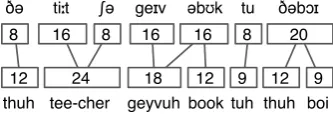
ðə tiːt geɪv əbʊk tu ðəbɔɪ

thuh tee-cher geyvuh book tuh thuh boi

ʃə

Figure 1: Aligning words from non-standard ortho-graphic transcriptions with the Gale-Church Algo-rithm, using normalised word lengths.

L2. P(#F|#E) is the prior probability of

align-ment between sentence sets of sizes _|F_| and _|E_|. The priors for alignment types used in the original algorithm are given in Table 1.

Then, for two paragraphs with numbers of sen-tences L1 and L2, their highest-probability

align-ment is derived using the following procedure. De-note the probability of the best alignment between the sentences 1... i_≤I and 1... j _≤J byP(i, j), and the alignment itself byB(i, j). ThenB(i, j) is determined by:

Application to transcription normalisation.

The GCA can be applied to align transcriptions at the level of words, rather than sentences, with-out violating the assumptions of the model (see Figure 1). In this way, the algorithm may be used to pre-process documents by splitting them into smaller pieces – aligned words – for further character-level processing such as alignment and transliteration.

The algorithm as defined is only applicable to aligning two sentences at a time. However, it has a simple extension to allow alignments of N tran-scriptions simultaneously. The best alignment be-tween sentences {1, ..., i1}, ..., {1, ..., iN} is

deter-where the distance function D is defined as an N-dimensional generalisation of the original GCA dis-tance function.

Limitations. The GCA only uses the

informa-tion about the lengths of the word fragments. Hence it ignores other useful information such as the characters used in the word fragments. A

tightly coupled character pair, e.g. characters cor-responding to a rare sound, may strongly indi-cate the true fragment alignment. In determin-ing the most likely alignment between sentences, the algorithm uses predefined prior probabilities of alignment types, based on European languages. In order to apply the algorithm to word fragment alignments, these prior probabilities should be re-estimated. Since the GCA is only applied to syn-thetic data in this work, we will retain the original priors and generate data according to them.

3.2 Moses

In order to perform a system-level evaluation of the GCA as a transcription pre-processor for character-based aligners, we require an established alignment system. For this purpose we use Moses, which is an SMT system designed to extend the IBM Models for unsupervised phrase-based trans-lation (Koehn, 2010).

Model description. Moses uses a mathematical

model to determine a probability distribution over possible translations of a sentence. Given a source language sentence e, a foreign language sentence f, and a division of the sentences into I phrases (blocks of consecutive words), the probability of the foreign sentence given the source sentence is defined as follows (Koehn, 2010):

p(fI|eI) = I Y

i=1

φ(fi|ei)d(starti−endi−1−1) (3.3)

where ei and fi are the ith phrases in the source and foreign languages, φ(f_|e) is the probability of translating the phrase e into f, starti is the po-sition of the first word in the ith phrase, endi is the position of the last word in theith phrase, and d is a function that penalises re-ordering (when starti−endi−1−16= 0).

Application to transcription problem. To

apply Moses to the transcription normalisation problem, we adopt the basic unit of characters in-stead of words. In this context, a “phrase” corre-sponds to a word fragment, or sequence of charac-ters.

The first step of Moses training uses GIZA++ (Och and Ney, 2003) to establish likely word ments. We use the HMM model for word align-ment (Vogel et al., 1996), since the IBM models encompass reorderings which are not relevant for transcription alignment. An example of training Moses to detect regular sound correspondences be-tween Portuguese and Spanish from a comparative wordlist (Wagner, 2010) is shown in Table 2.

4

HMM method

In this section a new method for transcription nor-malisation based on Hidden Markov Models is

ES PT φ(ES_|PT) N

ie e 0.72 50

rse r se 0.93 28

rs r se 0.81 32

´

on ˜ao 0.71 24

Table 2: Sample of results from training Moses on a Spanish-Portuguese comparative wordlist. φ is the proportion of instances of the ES fragment aligning with the PT fragment. N is the number of samples of the ES fragment.

troduced. This method aims to address the prob-lem of N-way transcription normalisation.

4.1 Model description

The leading idea in the new model is that whatever orthography is used, the sequence of characters in a transcription corresponds closely to the sequence of sounds heard by the transcriber. This suggests a model in which the characters are treated as emis-sions and the sounds are treated as hidden states in a modified version of a Hidden Markov Model. Our goal is to infer the most likely hidden state (sound) sequence given a set of N transcriptions of the same audio, and to use this as a normalised form.

Each hidden state (sound) is associated with a probability distribution over all possible emis-sions. Emissions are character sequences ranging in length from 0 up to some maximum, denoted LE. Hence, denoting the emission probability dis-tribution for hidden state elementsbyφs,

φs(e) : LE_[

i=0

{c1, c2, ..., cN}i→[0,1] (4.1)

where the_{ci_}is an inventory of all the characters used in the orthography.

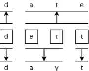
This setup would be sufficient if character emis-sions occur in a strict linear order with respect to the hidden states emitting them, but that is not al-ways true. A counter-example is given by the En-glish worddate. In Figure 2, the last three sounds together cause the emission ate: the emission of the charactereis unique to thecombination of the sounds. This phenomenon is not modelled suffi-ciently by, say, adding some probability of emitting the characterstefrom thetsound; the extra letter is only emitted when the sounds occur together.

To address this problem, we allow emissions from

blocks of hidden states acting in unison, referred to

assource blocksor justsources. A source block,

s, is defined by:

s_∈ LB [

i=1

{h1, h2, ..., hM}i (4.2)

Figure 2: Transcriptions of the word date using English orthography and a hypothetical phonetic orthography. The true sequence of sounds is shown in IPA in the center. The correspondence be-tween sounds and orthographic representation is indicated using arrows. Note that the last three sounds together are responsible for the emission of the charactersate in English orthography.

whereLBis the length of the longest source block allowed by the model, and the hi are the hidden states of the model, of which there areM in total. Each block has its own emission probability dis-tribution which treated as being independent from the emission distributions of its components. In Figure 2, the last three sounds act as a block in the top transcription language. Apart from block emissions, no other provisions are made for out-of-order emissions.

Given a set of N transcriptions assumed to be of the same audio, we can compute its probabil-ity with respect to a given hidden state sequence using the ideas of source blocks and emissions. A

model is a pair composed of a hidden state

se-quence S = h1, h2, ..., h|S| and analignment ψ of the state sequence to the characters in the tran-scriptions. The alignment is constructed by split-ting each transcription into emissions, and splitsplit-ting the hidden state sequence into source blocks, which are assigned to the emissions in order (hence, for each transcription, there must be an equal num-ber of source blocks and emissions). Note that the hidden state sequence may be split into source blocks differently for each transcription. Hence, the complete alignment is a vector of independent per-transcription alignments, ψ= (ψi). An align-mentψi of a hidden state sequence of length_|S_|to a particular transcription of lengthLiis defined as a vector of pairs (see Figure 3):

ψi= [([s1, s2),[t1, t2)),([s2, s3),[t2, t3)), . . . ,

([sJ,_|S_|),[tJ, Li+ 1))] (4.3)

where s1 = t1 = 1, J = |ψi| is the number of

source blocks, and ti may equal ti+1 in the case

of a zero-length emission. Then, the probability of an observed set of M transcriptions given a state

Alignment 1

Alignment 2 Hidden State Sequence

Transcription 2 Transcription 1

Figure 3: Sample alignment of a hidden state sequence of length 5 to two transcriptions. In transcription 1, sounds [2,3] emit characters [3,6] as a block, and in transcription 2, sounds [1,2] emit characters [1,2] as a block. The align-ment for Transcription 1 as defined in (4.3) is: ψ1 = (([1,2),[1,3)),([2,4),[3,7)),([4,5),[7,10)),

([5,6),[10,11))).

sequence and alignment is given by:

P(T1, T2, ...,TM|S, ψ) =

M Y

i=1

J Y

j=1

φi([tj, tj+1)|[sj, sj+1)) (4.4)

where we have definedφi_(e

|s) to be the probability of emitting the emission efrom the source blocks in theith transcription language. For the purpose of inferring the most likely hidden state sequence, we use Bayes’ Theorem: the probability of a model given a set of transcriptions is proportional to:

P(S, ψ|T1, T2, ...,TM)∝

P(S, ψ)P(T1, T2, ..., TM|S, ψ)

(4.5)

where to calculate P(S, ψ), we use a first order Markov Model on the hidden state sequence, and make no relative penalties for different alignments:

P(S, ψ) =P(S) = Y

(Si,Si+1)

P(Si+1|Si) (4.6)

4.2 Model Implementation

The model and an EM training procedure were im-plemented in C++.

Training. Training follows a modified

Expecta-tion MaximisaExpecta-tion format. The emission distribu-tions and bigram model for the hidden states are initialised randomly, then the following process is looped over a fixed number of iterations:

1. Model fitting:

(a) State sequences are sampled randomly for each sentence group in the corpus. (b) Random alignments to the transcriptions

are generated for each state sequence. (c) Probability of the random fits calculated. 2. Model re-estimation:

(a) Count for each emission event and state sequence event are weighted by probabil-ity of the sample in which they occur and added to running totals.

(b) Weighted counts for each event are nor-malised and smoothing is applied. (c) Pairs of sources with low information

radii are merged.

Sampling Strategy. We use a greedy sampling

strategy to ensure that some high likelihood mod-els are included in the sample. Specifically, the process is as follows:

1. Choose a random number of sounds for the state sequence.

2. Choose a (uniformly) random alignment to the transcriptions.

3. For each state sequence position, randomly se-lect sounds and evaluate the probability of the partial model.

4. Choose the sound that had the highest prob-ability.

The number of times random sounds are drawn in step 3 is equal to the number of hidden states used by the model. This ensures a good chance of a higher-probability sound being chosen, while preventing lower probability samples from being unrepresented.

Clustering. The last part of the E-step in the

main training procedure is a form of clustering. The two most similar source blocks (defined by similarity of their emission distributions) are com-bined. One source block takes on the average dis-tribution of the two, while the other is re-initialised with a uniform distribution. This leaves one source block free to acquire a new emission probability distribution, which may lead to a better overall modelling of the data. Hence, the clustering step provides a way for the training to jump out of lo-cal maxima. Clustering may be repeated a variable number of times, to merge multiple similar source pairs in a single training iteration. The similarity measure over emission distributions used to deter-mine which source pairs to merge is the informa-tion radius (Manning and Sch¨utze, 1999).

Length normalisation. Longer sentences

natu-rally correspond to longer state sequences. Hence there are more possible models for a longer sen-tence, and therefore the probability of any given model is lower. This reduces the weight associ-ated with a longer sentence when training. In fact, given two sentences, one twice as long as the other, the weight of the longer sentence will be roughly the square of the weight of the shorter one. Since the event counts are weighted by the probability of the sample containing them (and hence weights are<1), longer sentences will contribute less data

when training. This bias can be prevented using length normalisation. Length normalisation scales the weight of a sample according to its length. The length normalised weight for a sample is given by w∗₌ |S|√_{wwhere|S| is the length of the state}

se-quence and w is the model probability computed using Equation (4.4).

4.3 Limitations

While the hidden state sequence is a natural nor-malised form for transcriptions, it is not enlight-ening when inspected. Hidden states are labelled only by integers, hence there is no immediate indi-cation of what sound a particular hidden state may represent. Thus, a further decoding procedure may be needed to convert the true normalised form to a human-readable form.

Another limitation of the method is that it does not consider previously-known correspon-dences between transcription styles. For example, transcribers using similar character sets would be likely to use the same characters to mean the same sounds. The algorithm converts each data set into a list of integers, where each unique character has a single entry in a map. The maps for each transcrip-tion language are independent. Taking this type of information into account in advance may speed up the training process and improve its accuracy.

A further limitation is that the emission distri-bution associated with a source block is treated as being independent from the emission distributions of its constituent sounds. This is unrealistic; for example, if a source block in English contains the soundt, it is very likely that the emission produced by that source block will contain the letter t, but this is not captured in the model.

5

Evaluation

In the first sections we outline two synthetic data generation methods. These are designed to allow evaluation of character-based aligners based on the ground truth emission correspondences in the gen-erated corpora. A metric quantifying the differ-ence between the emission distributions learned by the character aligner and the ground-truth distri-butions is also defined. The evaluation is limited to the case of two parallel transcriptions. Evalua-tion of a character-based aligner involves an 18 part test performed for each data generation method: combinations of 3 sentence lengths (5, 10, and 15 words), and 3 corpus sizes (10, 25, 50 sentences), with and without GCA pre-processing of the cor-pus. Each test was performed 3 times with dif-ferent randomly generated corpora and the results were averaged to give the presented value.

The next section involves an evaluation of GCA for the purpose of pre-processing transcriptions for normalisation. For this purpose, we outline a

sim-ple data generation scheme to produce parallel cor-pora with known ground truth alignments. Fur-thermore, the efficacy of the GCA as a preproces-sor for character-based alignment tools is examined by studying the effect of GCA pre-processing on alignments learnt by the well-known Moses SMT system.

5.1 Synthetic method 1

This method is intended to produce corpora with character-aligned text in two randomly generated ‘languages’. First, a setEof random possible emis-sions are generated in the first language. For each emission e ∈ E, a probability distribution over emissions in the second language, φe(f), is ran-domly generated. The support of eachφe(f) distri-bution includes a small number of emissions, uni-formly chosen between 1 and 5.

To generate words, a random integer is chosen from a gamma distribution, and that number of emissions are drawn uniformly from the set E of possible emissions in the first language. For each emission e included in the word, a corresponding emission f is drawn from the φe(f) distribution. The emissions are concatenated to form the words. An alignment type is then drawn from the GCA priors (Table 1). The corresponding words are split according to the alignment type, where split points are chosen uniformly along the length of the words. Sentences are generated by stringing together se-ries of words generated in this way. Hence the true emission correspondence distributions φe are known and can be compared to those learnt by an aligner.

5.2 Synthetic method 2: Block-based

HMM

The second synthetic method involves generation of parallel corpora under the assumptions of the HMM method. This method may be used to gen-erate any number of transcriptions simultaneously, but for this application we limit generation to two languages at a time. The data generation process is as follows:

1. A random language model for hidden states is generated, a random set of valid source blocks is generated, and random emission distribu-tions for all valid source blocks are generated as in Synthetic Method 1.

2. For each individual word, a state sequence length is drawn from a gamma distribution. 3. For each word, a random sequence of sounds of

that length is generated according to the lan-guage model, with initial probabilities equal to the stationary probabilities of the chain. 4. Starting with the longest block length, LE,

and working back to blocks of length 1, emis-sions are chosen for any valid blocks appearing

in the state sequence.

5. The resulting emissions are concatenated to form the words for each transcription. 6. An alignment type is chosen from the GCA

priors and the words are split according to that alignment, uniformly along their length. 7. Words formed this way are strung together to

form sentences.

To calculate the true correspondence distributions between emissions we use Bayes’ Theorem. Let f be an emission in the second language, and e an emission in the first language. Then the probabil-ity of an instance of e corresponding to f in the corpus is:

P(f|e) =X s∈S

P(f, s|e)∝X s∈S

P(s)P(e|s)P(f|s)

(5.1)

WhereS is the set of possible source blocks. Note that emissions selected for the different transcrip-tions from a common source are independent, so that P(f|s, e) = P(f|s). Note also that the di-vision of the hidden state sequence into blocks is common to both transcription languages. To cal-culate Equation (5.1),P(e_|s) andP(f_|s) are taken directly from the emission distributions. P(s) is calculated using the stationary properties of the Markov chain used in sequence generation. Writ-ings=s1, s2, ..., sN, we have the approximation:

P(s) =α(s1)P(s1|s2)... P(sN−1|sN) (5.2)

whereα(s1) is the stationary probability of the first

sound of the source block. Equation (5.2) is only correct if word boundaries are treated as states in the HMM, which they are not; state sequence lengths are pre-drawn from a gamma distribution. However, the assumption becomes more accurate as the mean word length increases, and the aver-age source block length decreases. Keeping block lengths short (maximum of 2-sound blocks) mit-igates the effects of this inaccuracy, and the as-sumption will be kept.

5.3 Evaluation metric

For each of the data generation methods explained above, we have access to ground truth distributions for regular emission correspondences between the two languages. We define an accuracy metric based on the information radii between the true corre-spondence distributions (produced during corpus generation) and those produced by the aligners. Moses automatically produces emission correspon-dence distributions, and for the HMM method they are calculated using Equation (5.1).

Although information radius is only defined for two distributions, we can define a new metric quan-tifying the distance between a set of paired distri-butions. Let the paired distribution sets be {Pi}

Align P R F-score N

0 - 1 0.00 0.00 0.00 104

1 - 1 0.90 0.95 0.93 8886

1 - 2 0.82 0.67 0.74 893

2 - 2 0.00 0.00 0.00 117

Table 3: Results of running GCA on a corpus

and _{Qi_}, i_∈E, (E is the set of all emissions ob-served in the first language). Then we will use the metric:

D=X

i∈I

wiIRad(Pi, Qi) (5.3)

where IRad is the information radius (Manning and Sch¨utze, 1999), and the weightwi is the pro-portion of occurrences of the ith emission in the corpus, relative to all other emissions.

5.4 Gale-Church evaluation

For evaluation of the GCA, parallel corpora were generated using the following procedure:

1. A random sequence of alignments (0-1,1-1, etc.) was drawn with probabilities equal to the priors in the GCA (Table 1).

2. For each alignment, a random word length was drawn from a gamma distribution to form the first corpus. The parameters of the gamma distribution were chosen to be similar to those in the distribution of lengths of English words (West, 2008).

3. Each such word was randomly ‘translated’ un-der the assumptions of the GCA; the corre-sponding word length was drawn from a nor-mal distribution according to the assumptions of the GCA (Gale and Church, 1993). 4. Each word pair in both corpora was then

split according to their associated alignment type. Word splitting was distributed uni-formly along the length of the word.

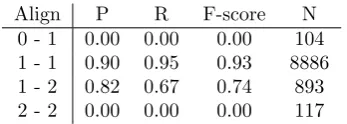
The parallel corpora generated were aligned using the unmodified GCA, and the accuracy of the re-sulting alignment was quantified using an F-score. Results of running the GCA on a corpus gen-erated using the above method are presented in Table 3. The algorithm did not correctly identify any 0-1 or 2-2 alignments. This effect occurs when aligning short (word size of less than 10 characters) fragments; increasing the word lengths to sentence size (_∼100 characters) causes the alignments to be picked up by the algorithm. The effect likely re-lates to the very low priors assigned to those align-ment types (see Table 1). On the other alignalign-ment categories, the algorithm performs well.

The results of running Moses on corpora gener-ated using synthetic methods 1 and 2 are shown in Tables 4 and 5 respectively. For both data gener-ation methods it is clear that pre-processing using

M/+G #Sentences

10 25 50

#W

ords

5 0.33/0.27 0.28/0.16 0.31/0.15 10 0.46/0.29 0.46/0.16 0.30/0.10

15 - /0.31 - /0.22 - /0.16

Table 4: Moses accuracy scores calculated using (5.3) (lower is better), for Synthetic Method 1. M: Moses alone, M+G: corpus pre-processed us-ing the GCA. A dash represents failure of Moses to train (common with long sentences).

M/+G #Sentences

10 25 50

#W

ords

5 0.18/0.06 0.05/0.03 0.03/0.03 10 0.29/0.04 0.18/0.01 0.32/0.05 15 0.28/0.03 0.33/0.04 0.21/0.02

Table 5: Moses accuracy scores calculated using (5.3) (lower is better), for Synthetic Method 2. M: Moses alone, M+G: corpus pre-processed us-ing the GCA.

GCA improves the ability of Moses to learn emis-sion correspondences. The effect of using GCA as a pre-processor is especially pronounced in the case of synthetic method 2, where dramatic decreases in the evaluation metric are observed. In addition to improving the accuracy of the training, the GCA also makes training possible on corpora which in-clude longer sentences.

5.5 HMM Method

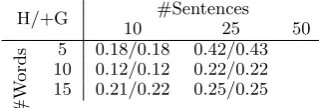
The results of running the HMM Method on cor-pora generated using synthetic methods 1 and 2 are shown in Tables 6 and 7 respectively. GCA pre-processing appears to have little effect on accuracy for this method. The method performs extremely well on corpora generated using synthetic method 2, which uses the assumptions of the HMM model. Comparing the results of training across the two data generation methods, it is clear that while the HMM method performs exceptionally on corpora generated using its assumptions, the implementa-tion cannot yet achieve similar results on corpora which are generated differently.

H/+G ₁₀ #Sentences_{25 50}

#W

ords

5 0.18/0.18 0.42/0.43 10 0.12/0.12 0.22/0.22 15 0.21/0.22 0.25/0.25

Table 6: HMM Method accuracy scores calcu-lated using (5.3) (lower is better), for Synthetic Method 1. H: HMM Method alone, H+G: corpus pre-processed using the GCA. Not all evaluations were completed due to prohibitive running times on large corpora.

H/+G #Sentences

10 25 50

#W

ords

5 0.00/0.00 0.00/0.00 10 0.00/0.00 0.00/0.00 15 0.00/0.00 0.01/0.01

Table 7: HMM Method accuracy scores calcu-lated using (5.3) (lower is better), for Synthetic Method 2. H: HMM Method alone, H+G: corpus pre-processed using the GCA. Not all evaluations were completed due to prohibitive running times on large corpora.

6

Conclusion

We have introduced the transcription normalisa-tion problem, and have tested the applicanormalisa-tion of new and existing computational methods to it, with mixed results.

The evaluation of the Gale-Church Algorithm showed that it has a significant positive impact on subsequent training of character aligners. Hence the GCA will be useful in preparing texts so that they may be subject to character level processing, such as alignment and transliteration.

Regrettably, the implementation of the HMM method could not be fully developed in the avail-able time. Features such as greedy sampling of the alignment space remain to be implemented. The method displayed promising results on corpora generated under HMM assumptions, however it is not yet versatile enough to achieve similar results when modelling corpora generated under different assumptions.

The results of the evaluation, while illustrating some interesting comparisons, are difficult to inter-pret. For instance, it is unclear what value of the accuracy metric a system would have to produce before it could be declared accurate enough to be useful in the transcription normalisation problem. Such investigations would require human evalua-tors.

Acknowledgements

We are grateful to David Chiang and three anony-mous reviewers for helpful comments on the work reported here.

References

Steven Abney and Steven Bird. 2010. The human language project: Building a universal corpus of the world’s languages. InProceedings of the 48th Annual Meeting of the Association for Computa-tional Linguistics, pages 88–97. Association for Computational Linguistics.

Jason Baldridge and Alexis Palmer. 2009. How well does active learning actually work? Time-based evaluation of cost-reduction strategies for language documentation. In Proceedings of the 2009 Conference on Empirical Methods in Nat-ural Language Processing, pages 296–305. Asso-ciation for Computational Linguistics.

William A. Gale and Kenneth W. Church. 1993. A program for aligning sentences in bilingual cor-pora. Computational Linguistics, 19:75–90.

Kevin Knight and Jonathan Graehl. 1998. Ma-chine transliteration. Computational Linguis-tics, 24.

Philipp Koehn. 2010. Statistical Machine Trans-lation. Cambridge University Press.

Michael E. Krauss. 2007. Mass language ex-tinction and documentation: the race against time. In Osahito Miyaoka, Osamu Sakiyama, and Michael E. Krauss, editors, The Vanishing Languages of the Pacific Rim. Oxford University Press.

Christopher D. Manning and Hinrich Sch¨utze. 1999. Foundations of Statistical Natural Lan-guage Processing. MIT Press.

Franz Josef Och and Hermann Ney. 2003. A sys-tematic comparison of various statistical align-ment models. Computational Linguistics, 29:19– 51, March.

Stephan Vogel, Hermann Ney, and Christoph Till-mann. 1996. HMM-based word alignment in statistical translation. COLING’96: The 16th International Conference on Computational Lin-guistics, pages 836–841, August.

Jennifer Wagner. 2010.

Ro-mance languages vocabulary lists.

http://www.ielanguages.com/romlang.html, December.

Marc West. 2008. The mystery of zipf.

http://plus.maths.org/content/mystery-zipf, August.

Anthony C. Woodbury. 2010. Language documen-tation. In Peter K. Austin and Julia Sallabank, editors,The Cambridge Handbook of Endangered Languages. Cambridge University Press.

Fei Xia and William D. Lewis. 2007. Multilin-gual structural projection across interlinearized text. InProceedings of the Meeting of the North

American Chapter of the Association for Com-putational Linguistics, pages 452–459. Associa-tion for ComputaAssocia-tional Linguistics.