ceiops calibration paper en

(1)

CEIOPS-SEC-40-10 15 April 2010

Q

I

S

5

C

(2)

Introduction

1.1 This paper provides background information to the technical analysis carried out by CEIOPS for the calibration of key parameters of the SCR standard formula and the calculation of technical provisions for the purpose of QIS5.1

2.

Technical provisions

2.1 Extrapolation of the risk-free interest rate term structure

2.1 For liabilities expressed in any of the EEA currencies, Japanese yen, Swiss franc, Turkish lira or USA dollar, QIS5 provides to participants risk-free interest rate term structures.

2.2 This subsection serves to give a rationale for the set up of the interest rate term structures for currencies where the relevant risk-free interest rate term structures are provided in the spreadsheet included in QIS5 package.

Basic Principles

2.3 According to the recommendation of the Task Force on the Illiquidity premium, the following principles are applied in constructing the extrapolated part of the basic risk free interest rate term structure:

#1. All relevant observed market data points should be used.

#2. Extrapolated market data should be arbitrage-free.

#3. Extrapolation should be theoretically and economically sound.

#4. The extrapolated part of the basis risk free interest rate curve should be calculated and published by a central EU institution, based on transparent procedures and methodologies, with the same frequency and according to the same procedures as the non extrapolated part.

1_{This document compiles information which has been published as part of the final advice on}

Level 2 Implementing Measures for Solvency II in the course of 2009 and 2010. For the overview of the Level 2 advice, please see:

(4)

#5. Extrapolation should be based on forward rates converging from one or a set of last observed liquid market data points to an unconditional ultimate long-term forward rate to be determined for each currency by macro-economic methods.

#6. The ultimate forward rate should be compatible with the criteria of realism as stated in CEIOPS advice on the risk free interest rate term structure and the principles used to determine the macro-economic long-term forward rate should be explicitly communicated.

#7. Criteria should be developed to determine the last observed liquid market data points which serve as entry point into the extrapolated part of the interest curve and for the pace of convergence of extrapolation with the unconditional ultimate long-term forward rate.

#8. Extrapolated rates should follow a smooth path from the entry point to the unconditional ultimate long-term forward rate.

#9. Techniques should be developed regarding the consideration to be given to observed market data points situated in the extrapolated part of the interest curve.

#10. The calibration of the shock to the risk free interest rate term structure used for the calculation of the SCR should be reviewed in order to be compatible with the relative invariance of the unconditional ultimate long-term forward rate.

Extrapolation method

2.4 For QIS5, macroeconomic extrapolation techniques are used to derive the extrapolation beyond the last available data point. The overall aim is to construct a stable and robust extrapolated yield curve which reflects current market conditions and at the same time embodies economical views on how unobservable long term rates are expected to behave. Macroeconomic extrapolation techniques assume a long-term equilibrium interest rate. A transition of observed interest rates of short-term maturities to the assessed equilibrium interest rate of long-term maturities takes place within a certain maturity spectrum.

2.5 Valuation of technical provisions and the solvency position of an insurer or reinsurer shall not be heavily distorted by strong fluctuations in the short-term interest rate. This is particularly important for currencies where liquid reference rates are only available for short term maturities and simple extrapolation of these short term interest rates may cause excessive volatility. A macro-economic model meets the demands on a model that ensures relatively stable results in the long term.

(5)

2.7 The specifications to be made are the following:

• Determination of the ultimate forward rate

• Interpolation method between the last observable liquid forward rate and the unconditional forward rate

Determination of the ultimate forward rate

2.8 A central feature is the definition of an unconditional ultimate long-term forward rate (UFR) for infinite maturity and for all practical purposes for very long maturities. The UFR has to be determined for each currency. While being subject to regular revision, the ultimate long term forward rate should be stable over time and only change due to fundamental changes in long term expectations. The unconditional ultimate long-term forward rate should be determined for each currency by macro-economic methods.

2.9 Common principles governing the methods of calculation should ensure a level playing field between the different currencies. For all currencies interest rates beyond the last observable maturity – where no market prices exist – are needed. One way to avoid creating an unlevel playing field when extrapolating the risk-free rate to time horizons of up to 100 years is to use for each currency all available market data from the liquid end of the term structure. 2.10 The most important economic factors explaining long term forward rates are

long-term expected inflation and expected real interest rates. From a theoretical point of view it can be argued that there are at least two more components: the expected term nominal term premium and the long-term nominal convexity effect.

2.11 The term premium represents the additional return an investor may expect on risk-free long dated bonds relative to short dated bonds, as compensation for the longer term investment. This factor can have both a positive and a negative value, as it depends on liquidity considerations and on preferred investor habitats: if investors seek higher returns for accepting the interest rate risk of long bonds it is positive, if they are prepared to accept a lower return in order to enjoy the advantages of a liability-matching investment, it will be negative.

2.12 The convexity effect arises due to the non-linear (convex) relationship between interest rates and the bond prices used to estimate the interest rates. This is a purely technical effect and always results in a negative component.

2.13 As no empirical data on the term premium for ultra-long maturities exists, the practical estimation of the term premium would be a challenging task and would involve extrapolating from the term premiums for lower maturities. 2.14 In order to have a robust and credible estimate for the UFR the assessment is

(6)

2.15 Making assumptions about expectations this far in the future for each economy is difficult. However, in practice a high degree of convergence in forward rates can be expected when extrapolating at these long-term horizons. From a macro economical point of view it seems consistent to expect broadly the same value for the UFR around the world in 100 years. Nevertheless, where the analysis of expected long term inflation or real rate for a currency indicates significant deviations, an adjustment to the long term expectation and thus the UFR has to be applied. Therefore, three categories are established capturing the medium UFR as well as deviations up or down.

Estimation of expected long term inflation rate

2.16 The expected inflation should not solely be based on historical averages of observed data, as the high inflation rates of the past century do not seem to be relevant for the future. The fact is that in the last 15-20 years many central banks have set an inflation target or a range of inflation target levels and have been extremely successful in controlling inflation, compared to previous periods.

2.17 Barrie Hibbert2_{propose to assess the inflation rate as 80 per cent of the}

globally prevailing inflation target of 2 per cent per anno and 20 per cent of an exponentially weighted average of historical CPI inflations when modelling the term structure in their Economic Scenario Generator. When they assess the historical inflation average of the main economies they still compute a high level as of December 2007 (they assess an expected global inflation rate of 2.4 per cent per anno) but with a strong downward trend over the sample of data they considered.

2.18 In order to have a robust and credible estimate for the UFR, the standard expected long term inflation rate is set to 2 per cent per anno, consistently to the explicit target for inflation most central banks operate with3_.

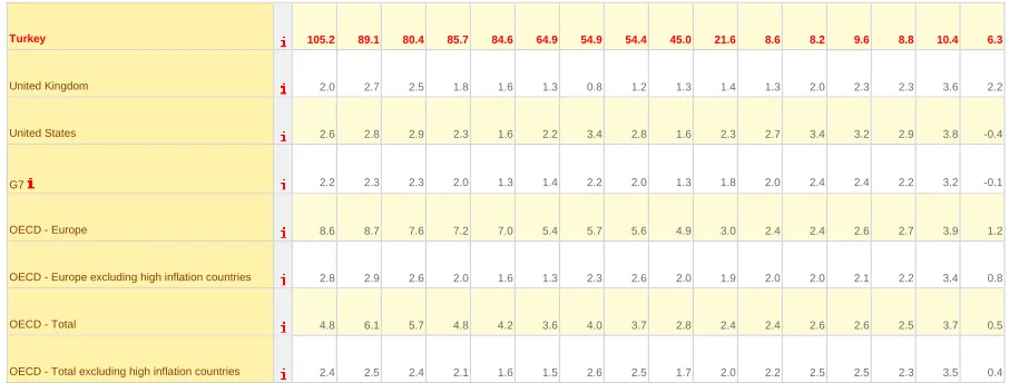
2.19 Nevertheless, based on historical data for the last 10-15 years and current inflation, two additional categories are introduced to capture significant deviations either up or down in the expected long term inflation rate for certain countries. Table 1 shows inflation data for the OECD-countries in the period 1994 – 2009.

Table 1: Inflation 1994 – 2009 OECD Countries

Price indices (MEI) : Consumer prices - Annual inflation Data extracted on 15 Mar 2010 13:35 UTC (GMT) from OECD.Stat

2_{Steffen Sørensen, Interest rate calibration – How to set long-term interest rates in the}

absence of market prices, Barrie+Hibbert Financial Economic Research, September 2008.

(7)

Measure Percentage change on the same period of the previous year

Frequency Annual

1994 1995 1996 1997 1998 1999 2000 2001 2002 2003 2004 2005 2006 2007 2008 2009

Time

Country

Australia 1.9 4.6 2.6 0.3 0.9 1.5 4.5 4.4 3.0 2.8 2.3 2.7 3.5 2.3 4.4 1.8

Austria 3.0 2.2 1.9 1.3 0.9 0.6 2.3 2.7 1.8 1.4 2.1 2.3 1.4 2.2 3.2 0.5

Belgium 2.4 1.5 2.1 1.6 0.9 1.1 2.5 2.5 1.6 1.6 2.1 2.8 1.8 1.8 4.5 -0.1

Canada 0.2 2.1 1.6 1.6 1.0 1.7 2.7 2.5 2.3 2.8 1.9 2.2 2.0 2.1 2.4 0.3

Czech Republic 10.0 9.1 8.8 8.5 10.7 2.1 3.9 4.7 1.8 0.1 2.8 1.9 2.6 3.0 6.3 1.0

Denmark 2.0 2.1 2.1 2.2 1.8 2.5 2.9 2.4 2.4 2.1 1.2 1.8 1.9 1.7 3.4 1.3

Finland 1.1 0.8 0.6 1.2 1.4 1.2 3.0 2.6 1.6 0.9 0.2 0.6 1.6 2.5 4.1 0.0

France 1.7 1.8 2.0 1.2 0.6 0.5 1.7 1.6 1.9 2.1 2.1 1.7 1.7 1.5 2.8 0.1

Germany 2.8 1.8 1.4 1.9 1.0 0.6 1.4 1.9 1.5 1.0 1.7 1.5 1.6 2.3 2.6 0.4

Greece 10.9 8.9 8.2 5.5 4.8 2.6 3.2 3.4 3.6 3.6 2.9 3.6 3.2 2.9 4.2 1.2

Hungary 18.9 28.3 23.5 18.3 14.2 10.0 9.8 9.1 5.3 4.7 6.7 3.6 3.9 8.0 6.0 4.2 Iceland 1.6 1.7 2.3 1.8 1.7 3.2 5.1 6.4 5.2 2.1 3.2 4.0 6.7 5.1 12.7 12.0 Ireland 2.4 2.5 1.7 1.4 2.4 1.6 5.6 4.9 4.6 3.5 2.2 2.4 3.9 4.9 4.1 -4.5

Italy 4.1 5.2 4.0 2.0 2.0 1.7 2.5 2.8 2.5 2.7 2.2 2.0 2.1 1.8 3.3 0.8

Japan 0.7 -0.1 0.1 1.8 0.7 -0.3 -0.7 -0.8 -0.9 -0.2 0.0 -0.3 0.2 0.1 1.4 -1.4

Korea 6.3 4.5 4.9 4.4 7.5 0.8 2.3 4.1 2.7 3.6 3.6 2.8 2.2 2.5 4.7 2.8

Luxembourg 2.2 1.9 1.2 1.4 1.0 1.0 3.2 2.7 2.1 2.0 2.2 2.5 2.7 2.3 3.4 0.4

Mexico 7.0 35.0 34.4 20.6 15.9 16.6 9.5 6.4 5.0 4.5 4.7 4.0 3.6 4.0 5.1 5.3

Netherlands 2.8 1.9 2.0 2.2 2.0 2.2 2.3 4.2 3.3 2.1 1.2 1.7 1.2 1.6 2.5 1.2

New Zealand 1.7 3.8 2.3 1.2 1.3 -0.1 2.6 2.6 2.7 1.8 2.3 3.0 3.4 2.4 4.0 2.1

Norway 1.4 2.4 1.2 2.6 2.3 2.3 3.1 3.0 1.3 2.5 0.5 1.5 2.3 0.7 3.8 2.2

Poland 33.0 28.0 19.8 14.9 11.6 7.2 9.9 5.4 1.9 0.7 3.4 2.2 1.3 2.5 4.2 3.8

Portugal 5.4 4.2 3.1 2.3 2.8 2.3 2.9 4.4 3.6 3.3 2.4 2.3 3.1 2.5 2.6 -0.8

Slovak Republic 13.4 9.8 5.8 6.1 6.7 10.6 12.0 7.3 3.1 8.6 7.5 2.7 4.5 2.8 4.6 1.6

Spain 4.7 4.7 3.6 2.0 1.8 2.3 3.4 3.6 3.1 3.0 3.0 3.4 3.5 2.8 4.1 -0.3

Sweden 2.2 2.5 0.5 0.7 -0.3 0.5 0.9 2.4 2.2 1.9 0.4 0.5 1.4 2.2 3.4 -0.3

(8)

Turkey 105.2 89.1 80.4 85.7 84.6 64.9 54.9 54.4 45.0 21.6 8.6 8.2 9.6 8.8 10.4 6.3

United Kingdom 2.0 2.7 2.5 1.8 1.6 1.3 0.8 1.2 1.3 1.4 1.3 2.0 2.3 2.3 3.6 2.2

United States 2.6 2.8 2.9 2.3 1.6 2.2 3.4 2.8 1.6 2.3 2.7 3.4 3.2 2.9 3.8 -0.4

G7 2.2 2.3 2.3 2.0 1.3 1.4 2.2 2.0 1.3 1.8 2.0 2.4 2.4 2.2 3.2 -0.1

OECD - Europe 8.6 8.7 7.6 7.2 7.0 5.4 5.7 5.6 4.9 3.0 2.4 2.4 2.6 2.7 3.9 1.2

OECD - Europe excluding high inflation countries 2.8 2.9 2.6 2.0 1.6 1.3 2.3 2.6 2.0 1.9 2.0 2.0 2.1 2.2 3.4 0.8

OECD - Total 4.8 6.1 5.7 4.8 4.2 3.6 4.0 3.7 2.8 2.4 2.4 2.6 2.6 2.5 3.7 0.5

OECD - Total excluding high inflation countries 2.4 2.5 2.4 2.1 1.6 1.5 2.6 2.5 1.7 2.0 2.2 2.5 2.5 2.3 3.5 0.4

2.20 Table 1 shows that two OECD-countries had inflation above 5 percent in 2009: Iceland (12 percent) and Turkey (6.3 percent). During the last 15 years, Turkey has been categorised by OECD as a high inflation country4_.

Turkey’s inflation target is also higher (5-7.5% for the period 2009 - 2012) than in other countries.

2.21 Based on this data basis, Hungary and Iceland are possible candidates for the high inflation group. However, deviations to the average inflation rate are far more moderate than those for Turkey. Furthermore, these countries are expected to join the Euro sooner or later (and thus have to fulfil the convergence criteria). Therefore, Hungary and Iceland are classified in the standard inflation category.

2.22 Japan, having deflation in the period since 1994, is an obvious candidate for the “low inflation”-group. Switzerland can also be seen as an outlier. This is due to the fact that historically relatively low inflation rates can be observed and that Switzerland is particular attractive in the international financial markets (exchange rate conditions, liquidity, “save haven”5_{...). For these}

reasons, lower inflation assumptions are applied for the Swiss francs.

2.23 The estimate covers one-year inflation rate 70 - 100 years from now. It is arbitrary to say whether the inflation differences we see today and have seen the last 15 years will persist 100 years into the future. However, historical evidence and current long term interest rates indicate that it is reasonable to have three groups of currencies with different inflation assumptions. The standard inflation rate is set to 2 per cent per anno. To allow for deviations up and down to the standard inflation rate, an adjustment to the estimate of +/- 1 percentage point is applied for the high inflation group and the low inflation group respectively. This adjustment of 1 percentage point will be applied to the estimated inflation rate for outliers based on differences in current long term interest rates (30Y), observed historical differences between the average interest rate and differences in short term inflation expectations.

4_{http://stats.oecd.org/index.aspx}

5 _{http://www.cepr.org/pubs/dps/DP5181.asp}_{”Why are Returns on Swiss Francs so low? Rare}

(9)

2.24 The following grouping is used for the estimated expected long term inflation rate:

• Standard inflation rate set to 2%: Euro-zone, UK, Norway, Sweden, Denmark, GBP, USD, Poland and Romania

• High inflation rate set to 3%: Turkey

• Low inflation rate set to 1%: Japan, Switzerland

Estimation of the expected real rate of interest

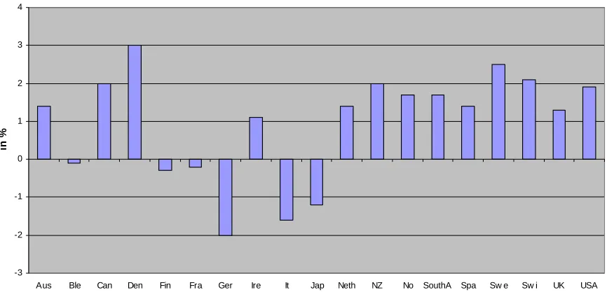
2.25 We expect that the real rates should not differ substantially across economies as far out as 100 years from now. Elroy Dimson, Paul Marsh and Mike Staunton provide a global comparison of annualized bond returns over the last 110 years (1900 to 2009) for the following 19 economies: Belgium, Italy, Germany, Finland, France, Spain, Ireland, Norway, Japan, Switzerland, Denmark, Netherlands, New Zealand, UK, Canada, US, South Africa, Sweden and Australia6_.

Figure 1: Real return on bonds 1900 – 2009

Source: Dimson, Marsh and Staunton – Credit Suisse Global Investment Returns Yearbook

-3 -2 -1 0 1 2 3 4

Aus Ble Can Den Fin Fra Ger Ire It Jap Neth NZ No SouthA Spa Sw e Sw i UK USA

in

%

2.26 Figure 1 shows that, while in most countries bonds gave a positive real return, six countries experienced negative returns. Mostly the poor performance dates back to the first half of the 20th_{century and can be}

6_{Credit Suisse Global Investment Returns Yearbook 2010, To be found at}

(10)

explained with times of high or hyperinflation7_{. Aggregating the real returns}

on bonds for each currency8_{to an annual rate of real return on globally}

diversified bonds gives a rate of 1.7 per cent.

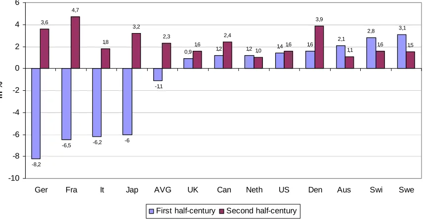
2.27 In an earlier publication, the same authors compared the real bond returns from the second versus the first half of the 20th_{century for the following 12}

economies: Italy, Germany, France, Japan, Switzerland, Denmark, Netherlands, UK, Canada, US, Sweden and Australia9_{. The average real bond}

return over the second half of the 20th_{century was computed as annually 2.3}

per cent (compared to -1.1 percent for the first half of the 20th_century).

Figure 2: Real bond returns: first versus second half of 20th_century*

Source: Dimson, Marsh and Staunton (ABN- Ambro/LBS)

-8,2

First half-century Second half-century

* Data for Germany excludes 1922-23. AVG = Average

2.28 In light of the above data, 2.2 per cent is an adequate estimate for the expected real interest rate.

7_{German hyperinflation in 1922/1923, in Italy an inflation of 344% in 1944, in France 74% in}

1946 and in Japan 317% in 1946.

8_{Average where each return is weighted by its country’s GDP.}

9_{Elroy Dimson, Paul Marsh and Mike Staunton: Risk and return in the 20th and 21th, Business}

Strategy Review, 2000, Volume 11 issue 2, pp 1-18. See Figure 4 on page 5. The article can be downloaded at:

(11)

Conclusion

2.29 In light of the above analysis, the macro economically assessed UFR for use in the QIS5 is set to 4.2 per cent (+/-1 percentage points) per anno. This value is assessed as the sum of the expected inflation rate of annually 2 per cent (+/- 1 percentage points) and of an expected short term return on risk free bonds of 2.2 per cent per anno.

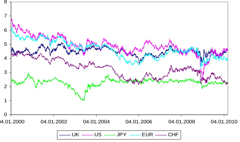
2.30 As we can see in figure 3, the development of long term interest rates for the last 10 years supports the proposed differentiation between Euro, GBP, USD in one group and JPY and CHF in another group.

Figure 3: Long term interest rates (30Y) – Source: Bloomberg

0 1 2 3 4 5 6 7 8

04.01.2000 04.01.2002 04.01.2004 04.01.2006 04.01.2008 04.01.2010

UK US JPY EUR CHF

2.31 Therefore, for QIS5 the following UFR are used:

Category Currencies Macro economically assessed UFR

(%)

1 JPY, CHF 3.2

2 Euro, SEK, NOK, DKK, GBP, USD,

PLN, RON, HUF, ISK

4.2

(12)

Specification of the transition to the equilibrium rate

2.32 This paragraph considers the issue of how to extrapolate between the estimated forward rates and this unconditional ultimate forward rate, i.e. the question which technique would be the most appropriate to use for all economies.

2.33 Two possible techniques, the linear extrapolation technique as proposed in Annex E of CEIOPS-DOC-34-09 (former CP40) and the Smith-Wilson technique are described below. The technical details for both techniques can be found in the Appendix A.

2.34 For both methods the term structure is fitted exactly to all observed zero coupon bond prices from the liquid market, i.e. all liquid market data points are used without smoothing. The term structure passes through all zero coupon market rates and this can therefore lead to a somewhat bumpy term structure curve in the liquid end of the data for both techniques.

2.35 In the linear interpolation technique the forward rates between the last observable forward rate at maturity T1 and a predefined maturity T2 are

interpolated linearly. In the Smith-Wilson approach kernel-functions (as many as data points) are defined and the term structure is computed as a linear combination of these kernel functions. The method is based on the assumption that the forward rates converge asymptotically to the UFR at the long end of the term structure. The speed of the convergence can be controlled by choosing an adequate parameter α.

2.36 One of the main differences between the two techniques is that in the linear extrapolation a fixed maturity T2 has to be assumed at which the

unconditional ultimate forward rate will be reached, while in the Smith-Wilson technique the assumption made is on how fast the forward rates converge to the unconditional ultimate forward rate.

2.37 There is no fixed, predefined maturity where the UFR is deemed to be arrived at in the Smith-Wilson approach. But the problem still remains on how to choose the speed of convergence. Thomas10_proposes_α_{= 0.1 for sensible}

results. The parameter is empirically fitted to give economically appropriate curves.

2.38 Another difference is that in the Smith-Wilson approach both interpolation (for maturities in the liquid end of the term structure where risk-free zero coupon rates are missing) and extrapolation are achieved, while we have to make an additional decision on how to deal with interpolation in the linear method. 2.39 The linear interpolation technique is a simple, extremely intuitive method,

easy to explain and easy to apply, but per definition does not give a smooth extrapolated forward curve (forward rate curve is only continuous, but not

10_{Michael Thomas, Eben Maré: Long Term Forecasting and Hedging of the South African Yield}

(13)

differentiable in T2.) The term structure however is differentiable in all

extrapolated points.

2.40 Furthermore, the linear interpolation method is sensitive to the values of the last two forward rates and includes expert opinion when setting the maturity of the UFR.

2.41 The Smith-Wilson approach is more sophisticated but still easy to use (in order to assess the term structure nothing else than an excel-sheet is needed), and gives both a relative smooth forward rate and a smooth spot rate curve in the extrapolated part. It was therefore decided to use the Smith-Wilson approach for extrapolating the interest rate curve in QIS5.

2.42 Nevertheless, alpha will be calibrated to ensure that the extrapolated curve is sufficiently close to the chosen UFR at T2. Furthermore, the linear method has been also run in order to provide a kind of cross-checking, avoiding a full reliance in a single method and enhancing the robustness of results provided by the Smith-Wilson approach.

Transition to the equilibrium rate – Smith-Wilson technique

2.43 The Smith-Wilson approach is a macroeconomic method: a spot (i.e. zero coupon) rate curve is fitted to observed bond prices with the ultimate long term forward rate as input parameter.

2.44 In its most general form, the input data for the Smith-Wilson approach can consist of a large set of different financial instruments relating to interest rates. We will limit the input to zero coupon bond prices, and will only put down the formulae for this simple case.

2.45 In other words: we assume that in the liquid part of the term structure the risk-free zero coupon rates for all liquid maturities are given beforehand. Our task is to assess the spot rate for the remaining maturities. These are both maturities in the liquid end of the term structure where risk-free zero coupon rates are missing (interpolation) and maturities beyond the last observable maturity (extrapolation).

2.46 Let’s assume that we have market zero coupon rates for J different maturities: u1, u2, u3, and so on. The last maturity for which market data is

given is uJ.

2.47 The market price P(t) for a zero coupon bond of maturity t is the price, at valuing time t0 = 0, of a bond paying 1 at some future date t. Depending on

whether the market data spot rates are given as continuously compounded rates

R with annual compounding, the input zero bond prices at maturities uj are:

P

=

−

for continuously compounded rates, and

(14)

The relation between the two rates is given through

ln(

1

~

)

j

j u

u

R

=

+

.

2.48 Our aim is to assess the function P(t) for all maturities t, t > 0. From the definition of the price function P(t)=exp(−t*R~_t) for continuously compounded

rates and

P

(

t

)

=

(

1

+

R

_t

)

-t for annual compounding, we then can assess the

whole risk-free term structure at valuing date t0 = 0.

General on extrapolation technique

2.49 Most extrapolation methods start from the price function, and assume that the price function is known for a fixed number of say J maturities. In order to get the price function for all maturities, some more assumptions are needed. 2.50 The most common procedure is to impose – in a first step - a functional form

with K parameters on the price function P11_{. These functional forms could be}

polynomials, splines, exponential functions, or a combination of these or different other functions12_.

2.51 In some of the methods, in a second step, the K parameters are estimated via least squares at each point in time. In other methods K equations are set up from which the K parameters are calculated. The equations are set up in a manner that guarantees that P has the features desired for a price function: A positive function, with value 1 at time t=0, passing through all given data points, to a certain degree smooth, and with values converging to 0 for large t.

Smith-Wilson approach

2.52 Smith and Wilson1314_{proposed a pricing function (here reproduced in a}

restricted form, only for valuing at point t0 =0) of the following form:

∑

11_{In their respective models, Svensson for instance imposes a parametric form with 6}

parameters and Nelson-Siegel one with 4 parameters.

12_{BarrieHibbert use cubic splines in the liquid part of the term structure and Nelson-Siegel for}

the extrapolation part.

13_{Smith A. & Wilson, T. – “Fitting Yield curves with long Term Constraints” (2001), Research}

Notes, Bacon and Wodrow. Referred to in Michael Thomas, Eben Maré: “Long Term Forecasting and Hedging of the South African Yield Curve”, Presentation at the 2007 Convention of the Actuarial Society of South Africa

14_{Andrew Smith: Pricing Beyond the Curve – derivatives and the Long Term (2001),}

presentation to be found at

(15)

{

*

min(

,

)

0

.

5

*

(

)

}

2.53 The following notation holds:

• J = the number of zero coupon bonds with known price function

• ui, i=1, 2, … J, the maturities of the zero coupon bonds with known prices

• τ = term to maturity in the price function

• UFR = the ultimate unconditional forward rate,

• α = mean reversion, a measure for the speed of convergence to the UFR

They depend only on the input parameters and on data from the input zero coupon bonds. For each input bond a particular kernel function is computed from this definition. The intuition behind the model is to assess the function P(t), from which we aim to calculate the term structure, as the linear

combination of all the kernel functions. This reminds of the Nelson-Siegel method, where the forward rate function is assessed as the sum of a flat curve, a sloped curve and a humped curve, and the Svensson method, where a second humped curve is added to the three curves from Nelson-Siegel. 2.55 The unknown parameters needed to compute the linear combination of the

kernel functions, ζi, i= 1, 2, 3 … J are given as solutions of the following linear

system of equations:

∑

2.56 In vector space notation this becomes:

(16)

,

calculated by inverting the JxJ-matrix (W(ui, uj)) and multiplying it with the

difference of the P-vector and the E-vector, i.e.

),

get the value of the zero coupon bond price for all maturities τ, for which no zero bonds were given to begin with:

∑

2.59 From this value it is straightforward to calculate the spot rates by using the definition of the zero coupon bond price. The spot rates are calculated as

)

R = for continuous compounded rates and

)

1

)

annual compounding is used.

Transition to the equilibrium rate – Linear extrapolation technique

2.60 Interpolation between market data points in the liquid part of the term structure

• Choose reference rates from market data according to the criteria for risk free rate specified in CP40.

• If the market data includes coupon payments, transform the data to zero coupon rates (spot rates) for every reasonably liquid maturity point given as yearly interval of 1, 2, 3,…,years. See specification on risk-free rates.

• Forward rates are calculated from the spot rates. Forward rates are the rates of interest implied by spot rates for periods of time in the future. If RS and RT are spot rates for maturities S and T, then the average annual

forward rate FR(S,T) for the period from S to T is defined by

(17)

• If no reliable rates are available for maturity points between e.g. liquid market data for maturities S and T, the intervening zero coupon rates have to be determined based on an additional assumption.

• In QIS4 this additional assumption was that forward rates between S and T are constant, i.e.

• In QIS5 (this is now implemented in the Extrapolator) the additional assumption is that the intervening spot rates can be determined by linear interpolation from RS and RT, the known spot rates for maturities S

and T

2.61 Extrapolation beyond the last liquid data point

• To be able to extrapolate, we have to define two specific points in time:

o T1 = the maturity of the last observed liquid spot rate (that meets

all the criteria)

o T2 = starting point for the ultimate unconditional long term forward

rate (UFR).

o The last observable market forward rate FR(T1-1) = FR(T1-1, T1) is

calculated from the last market data points.

• A constant ultimate unconditional forward rate UFR is applied for all maturities beyond T2. The method to determine this rate and the

maturity points T1 and T2 can differ between different currencies.

• Linear interpolation is used to arrive at one year forward rates FR(n) for maturities n between T1 and T2:

one year forward rate curve by

(18)

2.2 Cost-of-Capital rate

15

A general approach for stipulating the Cost-of-Capital rate

2.62 According to Article 77(5) of the Level 1 text the Cost-of-Capital rate “shall be the same for all insurance and reinsurance undertakings and shall be reviewed periodically”. Moreover, the Cost-of-Capital rate used

shall be equal to the additional rate, above the relevant risk-free interest rate, that an insurance or reinsurance undertaking would incur holding an amount of eligible own funds, […], equal to the Solvency Capital Requirement necessary to support the insurance and reinsurance obligation […].

2.63 As the “additional rate, above the relevant risk-free interest rate” referred to in Article 77(5) shall be the same for all insurance and reinsurance undertakings, it should be calibrated in a manner that is consistent with the assumptions made for the reference undertaking. In practise this means that the Cost-of-Capital rate should be consistent with the Value-at-Risk-assumption corresponding to a confidence level of 99.5 per cent over the stipulated one-year time horizon as laid down for the calculation of the Solvency Capital Requirement (SCR). Especially, the Cost-of-Capital rate should be independent of the actual solvency position of the original undertaking.

2.64 In the third and fourth Quantitative Impact Study for Solvency II (QIS3 and QIS4) the Cost-of-Capital rate had been fixed at 6 per cent as such a rate has been assumed to reflect the cost of holding an amount of eligible own funds for an insurance or reinsurance undertaking being capitalised corresponding to a confidence level of 99.5 per cent Value-at-Risk over a one year time horizon.

2.65 The required consistency between the stipulated Cost-of-Capital rate and the (Value-at-Risk) assumptions for the SCR-calculations was explained as follows: the 6 per cent Cost-of-Capital rate corresponds to the cost of providing eligible own funds for BBB-rated insurance or reinsurance undertakings, cf. the Cost-of-Capital rate used by the Swiss regulator in its Solvency Test for BBB-rated reference undertakings.

2.66 As part of the QIS4-feedback, questions have been raised regarding the appropriateness of the assumed Cost-of-Capital rate of 6 per cent. Especially, reference was made to the work carried out by the Chief Risk Officer Forum (CRO Forum), and a substantially lower Cost-of-Capital rate has been indicated.

(19)

2.67 However, a critical analysis of the CRO Forum’s report16_{– as well as other}

reports on this issue17_{– does not support the QIS4-feedback referred to}

above. On the contrary, the analysis which is summarised in the subsection below, indicates that an assumed Cost-of-Capital of 6 per cent or higher could be seen as appropriate – given the information currently available regarding this issue. In this context it should be noted that although the CRO Forum has indicated in its report that its research suggests a Cost-of-Capital rate in the range of 2 ½ - 4 ½ per cent, it also acknowledges that its research did not prove conclusive. Moreover, it seems that the CRO Forum first and foremost has focussed on results leading to the lowest estimates of the Cost-of-Capital rate.

2.68 The analysis summarised in the following subsection does not discuss the required periodical review as referred to in Article 77(5) of the Level 1 text. However, CEIOPS points out that the frequency and procedures to be followed for this review would need to be developed. A possible approach could be to test the appropriateness of the Cost-of-Capital rate every five years. In this context, it should be stressed that due to the long-term nature of the Cost-of-Capital rate, this does not necessarily mean that the rate has to be changed as a consequence of a periodic review.

Assessment of the Cost-of-Capital Rate

(a) Introductory remarks

2.69 The Cost-of-Capital rate is an annual rate applied to a capital requirement in each period. Because the assets covering the capital requirement themselves are assumed to be held in marketable securities, this rate does not account for the total return but merely for the spread over and above the risk free rate.

2.70 The risk margin shall guarantee that sufficient technical provisions for a transfer are available even in a stressed scenario. Hence, the Cost-of-Capital rate has to be a long-term average rate, reflecting both periods of stability and periods of stress. Otherwise, the rate would vary from year to year, and would be higher in times of economic uncertainty (when providers of capital would be expected to seek greater returns for the comparatively higher risk) and would therefore contribute to higher technical provisions than in more stable economic situations.

16_{CRO Forum: Market Value of Liabilities for Insurance Firms – Implementing Elements for}

Solvency II (July 2008).

17_{GNAIE (Group of North American Insurance Enterprises): Market Value Margins for}

Insurance Liabilities in Financial Reporting and Solvency Applications (October 2007),

(20)

2.71 A rate of at least 6 per cent is assessed to be an adequate placeholder for the Cost-of-Capital rate in the current context of the Solvency II regulation. In order to reach this conclusion it may be argued along the following lines:

• Shareholder return models provide the initial input.

• Some objective criteria may cause upward and downward adjustments of the initial input.

• A final calibration of the Cost-of-Capital rate, in order to obtain risk margins consistent with observable prices in the marketplace, may be necessary.

Before discussing this three-step procedure, it will be reflected on the assumptions that would be reasonable to make regarding the funding of the capital requirement.

(b) Funding of the capital requirement

2.72 In CRO Forum’s report, the Cost-of-Capital rate is calculated as a weighted average of the cost of equity and the cost of debt. It is assumed that 20 per cent of the capital requirement can be funded by issuing debt and that only the remaining 80 per cent have to be funded by raising equity capital. Moreover, by assuming an effective company rate of taxation of 35 per cent over all jurisdictions, the estimated cost of debt is in practise outweighed by the adjustments for tax relief on interest payments made to service the debt. As a result the Cost-of-Capital rate equals only approximately 80 per cent of the estimated cost of equity rate.

2.73 It should be noted that the assumed funding based on 80 per cent equity and 20 per cent debt cannot be justified in light of the feedback received during the QIS4-exercise. According to the QIS4-report the participating undertakings reported that 95 per cent of their own funds are classified as tier 1 capital of which only 2 per cent are classified as “subordinated loans” and only 4 per cent as “other reserves (with restricted loss absorbency)”. Moreover, only 50 per cent of the tier 2 and tier 3 capital are classified as subordinated loans or other hybrid capital.18_{Consequently, the QIS4-results}

indicate clearly that the assumed debt-funding in any case cannot constitute more than 6-8 per cent of the capital base.19

2.74 Moreover, it may be referred to the high-level political guidance to increase the quality of the external funding (subordinated loans, hybrid capital instruments etc.) of financial institutions. It follows from this that subordinated loans and hybrid capital should have a high loss-absorbing capacity rather similar to “core” capital, cf. the revision carried out in the

18 _{Cf. CEIOPS’ Report on its fourth Quantitative Impact Study (QIS4) for Solvency II, page}

129-132.

19_{In the remainder of the present sub-section it is referred to “the capital base” and not “the}

(21)

banking sector. Accordingly, it seems reasonable to expect the cost-differences between equity funding and allowed external funding to diminish. 2.75 In this context it should also be stressed that since the capital base is defined

as the solvency capital requirement in an adverse situation, i.e. as the amount of capital that is substantially at risk, it would be inconsistent to assume at the same time that this requirement can be funded by debt investors at costs substantially below equity.

2.76 With respect to the assumed impact of taxation (i.e. the tax relief on interest payments) on the assessment of the Cost-of-Capital rate, this aspect will be less important than assumed in CRO Forum’s report due to the QIS4-feedback referred to above.20_{However, it still remains to decide on the tax rate(s) to}

be used if a more detailed analysis of this aspect of the Cost-of-Capital calculations should be carried out.21

2.77 Based on the considerations given in the previous paragraphs CEIOPS finds that an approach based on the market situation (i.e. the actual combination of equity and debt funding) leads to conclusions similar to an approach based on 100 per cent equity funding. This is in particular the case for the purpose of the assessments summarised below.

(c) The three-step procedure for assessing the Cost-of-Capital rate

(c1)Shareholder return models

2.78 The research carried out by both CRO Forum and GNAIE has been analysed. As the most commonly used models in the market seem to be the Capital Asset Pricing Model (CAPM) and versions of the Fama-French multi Factor Model (FFmF), CEIOPS’ analysis has been confined to the results given for these models.

• The Frictional Cost-of-Capital approach

2.79 In CRO Forum’s research the rate of return above the risk free rate that shareholders of insurance undertakings demand in order to assume broadly diversified insurance risks, are estimated using different methods and assumptions. CRO Forum deems that the so-called Frictional Cost of Capital approach is the most appropriate to capture the rate of return an insurance company requires on the capital it deploys to support non-hedgeable risk over

20 _{A rather peculiar – and likely unintended – implication of the assumptions made in CRO}

Forum’s report should be mentioned. Since the estimated cost of debt is outweighed by the tax-relief on interest payments made to serve this debt, a logical conclusion seems to be that by increasing the (relative) debt-funding an insurance undertaking will be rewarded by a lower Cost-of-Capital rate. According to CEIOPS’ understanding this cannot be in line with the intention of Article 77(5) of the Level 1 text.

21_{It may also be questionable whether an insurance undertaking being in a stressed situation}

(22)

a given year. This is likely the reason why they rely so heavily on the results from this method when drawing their conclusions.

2.80 However, CEIOPS has reservations regarding the results based on this approach22_{as reproduced in the CRO Forum’ report. Firstly, the results of the}

method are very dependent on a number of key assumptions – effective tax rate, loss carry forward period and risk free rate – for which it is difficult to assess reasonable parameter estimates in an EU context. Secondly, of the main components of the frictional costs – double taxation costs, financial distress costs23_{and agency costs}24_{– only the two first have been modelled.}

2.81 Moreover, the CRO Forum has drawn e.g. the following conclusions after having modelled double taxation and financial distress costs:25

For highly capitalized companies, the cost of capital rate is determined mainly by the cost of double taxation and the cost of financial distress is negligible. […]

The cost of capital rate depends linearly on a jurisdiction’s tax rate for all confidence levels. This means that the cost of capital rate (and therefore the MVM) in a jurisdiction with a tax rate of 10% is only half of that in a jurisdiction with a tax rate of 20%.

In CEIOPS’ opinion the result implied by these conclusions does not seem reasonable for Member States in which the effective tax rate is low. Furthermore, CEIOPS also questions the assertion that financial distress costs are negligible for well capitalized companies.

• The CAPM and the FF2F-method

2.82 In CRO Forum’s research related to the CAPM and the FF2F method, the cost of equity rate above the risk-free rate has been estimated for three markets: the European, the Asian and the US market. From these estimated rates a “Global World” rate has been derived for both methods. The Global World rates are in general lower than the European rates, cf. table 2 below.26_When

concluding on an appropriate level of the Cost-of-Capital rate, CRO Forum has

22_{Under this approach, the total return required by shareholders may be thought of consisting}

of the base cost of capital, the frictional costs and the expected economic profit. Only the frictional costs are taken into account in determining the Cost of Capital rate.

23 _{These are direct and indirect costs which arise when an insurer has difficulties meeting its}

financial obligations to policyholders or debt holders.

24_{Agency costs are associated with the misalignment of the interest between management}

and shareholders or between policyholders and shareholders. The lack of transparency and informational asymmetry are also deemed to be part of agency costs.

25_{Cf. CRO Forum's report, page 36.}

26_{In the CAPM-case the reported Global rates are lower than the reported rates for all three}

(23)

taken into account only the lower Global World rates without giving any explicit rationale for this choice.

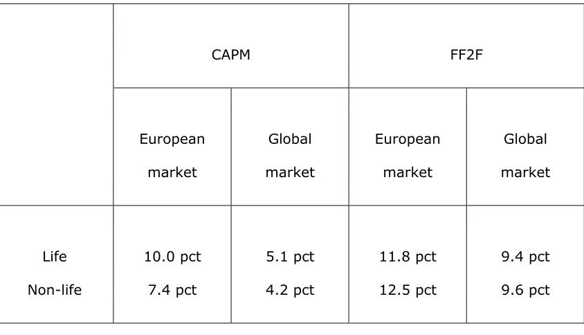
2.83 CEIOPS finds it more appropriate to base the assessment of the Cost-of-Capital rate on CRO Forum’s results for the CAPM and the FF2F method for European insurance undertakings. In this context it may also be noted that the FF2F-results for the European non-life insurers are in line with the results referred to in GNAIE’s report for US non-life insurers (an equity risk premium of 14.2 per cent).

Table 2. Equity Risk Premiums as assessed in the CRO Forum’s report.27

CAPM FF2F

European Global European Global

market market market market

Life 10.0 pct 5.1 pct 11.8 pct 9.4 pct

Non-life 7.4 pct 4.2 pct 12.5 pct 9.6 pct

2.84 Taking into account only the results from the shareholder return models a Cost-of-Capital rate of 7 ½-10 per cent seems to be adequate. It should, however, be noticed that the figures reproduced in table 2 are based on historical averages during normal times only and do not take into account stressed scenarios in an adequate manner.

(c2) Adjustment of shareholder return

2.85 To the output from the shareholder return models both upward and downward adjustments are needed when assessing the cost of capital rate in a solvency context.

2.86 Downward adjustments: In order to account for the fact that a key source of return that exists for going concerns (the so called franchise value related to expected profit from new business) may not be demanded by capital

(24)

providers in a transfer context, a downward adjustment is needed. No reliable quantitative results are available concerning the size of this adjustment.

2.87 Upward adjustments: Additional costs, i.e. costs beyond those required to compensate investors for the risk they are assuming, make an upward adjustment necessary. These additional costs may stem from:

• Frictional costs of carrying capital. These are additional costs28_which

reflect a variety of indirect costs, as frictional costs related to managers’ incentives, information asymmetries, and so on. Again, these costs are very difficult, if not impossible, to quantify.

• Initial costs of raising capital. These are fees for underwriting, listing and regulation, which in most jurisdictions are not negligible29_.

• Corporate income taxes on the risk margin in some tax jurisdictions. This is the case if the risk margin is considered as taxable profit at inception and not as taxable income only over the time of its release from the risk margin.

2.88 As already indicated, the aggregate effect of both upward and downward adjustments is difficult to quantify in a reliable manner. However, as it is unlikely that the downward adjustment outweighs the upward adjustments by a large margin, a range for the Cost-of-Capital rate after these adjustments of 6-8 per cent could be deemed as reasonable given the current market situation/information.

(c3) Calibration to market prices

2.89 The output for the cost of capital rate has to be calibrated further to give final risk margins consistent with observable prices in the marketplace. The risk margin together with the best estimate shall be “equivalent to the amount insurance and reinsurance undertakings would be expected to require in order to take over and meet the insurance and reinsurance obligations” (Article 77(3)).

2.90 In the Solvency II context an allowance may be necessary for the metho-dologies applied when calculating the capital base (i.e. the future SCRs). This is especially the case for any simplifying methods allowed.30_{All other}

assumptions equal, especially for unchanged best estimate, it may be argued that the cost of capital rate should be set higher if methods used in the solvency context give systematically lower capital bases than the capital

28_{Cf. the GNAIE-report, page 30.}

29 _{Underwriting fees, which generally constitute at least half of the direct IPO costs, amount to}

about 3.5% of the raised equity in the UK, Germany or France, and to more than 6.5% in the USA. Source: Oxera report (2006), “The Cost of Capital: An International Comparison”.

Available at www.oxera.com.

30_{In QIS4 a majority of undertakings (independently of their size) used simplifications when}

(25)

bases assessed through the markets in real insurance portfolio transfers. Otherwise the technical provisions will be insufficient.

2.91 As long as the method used in assessing the capital base does not systematically underestimate the needed amount, a Cost-of-Capital rate of 6 per cent could be seen as adequate. In order to avoid procyclical effects, the Cost-of-Capital rate should not be adjusted to follow market cycles.

2.3 Simplified calculation of the Risk Margin

2.92 Similarly to QIS4, CEIOPS' proposal for QIS5 specifications contains the following table for the case where it is possible to calculate the risk margin using the simple method based on percentages of the best estimate:

Line of Business Percentage of

Best Estimate

Direct insurance and accepted proportional reinsurance:

Accident 12.0 %

Sickness 8.5 %

Workers’ compensation 10.0 %

Motor vehicle liability 8.0 %

Motor, other classes 4.0 %

Marine, aviation and transport 7.5 %

Fire and other damage 5.5 %

General liability – Third party liability 10.0 %

Credit and suretyship 9.5 %

Legal expenses 6.0 %

Assistance 7.5 %

Miscellaneous non-life insurance 15.0 %

Accepted non-proportional reinsurance:

Property business 7.0 %

Casualty business 17.0 %

Marine, aviation and transport

business 8.5 %

2.93 The proposed percentages are based on table 69 of the QIS4 report, Annex of selected tables, pages A-74 to A-76, line ‘Life+Nonlife+Composites) (see

(26)

2.94 For almost all lines of business, the ratio observed in QIS4 does not show a significant standard deviation around the average ratio. Then and directly, the rounded percentage shown in the aforementioned table has been adopted as proposal.

2.95 Notwithstanding, there are three lines of business where the ratio observed in QIS4 has been considered not usable for the purposes of QIS5. In these cases the same percentages as QIS4 have been maintained, since there is no evidence of any practical problem derived from their application during that exercise.

2.96 The three lines of business where the same percentage as QIS4 is proposed, are:

i) Accident (due to the fact that in QIS4, data concerning this guarantee are embedded in various lines of business, and therefore no isolate and purely specific average ratio is available)

ii) Motor, other class (due to specific heterogeneity in the data provided from some markets, specifically analyzed and identified)

iii) Miscellaneous (due to its obvious heterogeneity)

3.

Solvency capital requirement: standard formula

3.1 Market risk

3.1.1 Interest rate risk

31

3.1 The calibration of the standard formula interest rate capital charge is based on the delta-NAV approach proposed in CEIOPS-DOC-40/09 (former CP47).

3.2 In CEIOPS-DOC-40/09, CEIOPS set out the capital charge arising from this

sub-module, termed Mktint, to be based on two pre-defined factors, an upward and downward shock in the term structure of interest rates combined with specific alterations in the interest rate implied volatility. The combination of the instantaneous shift of these factors yields a total of four pre-defined scenarios.

3.3 The first two scenarios will consider an upward shock to interest rates, whilst implied volatility experience an upward and downward parallel shift and will deliver MktintUpivolUp and MktintUpivolDn. The last two scenarios will consider a downward shock to interest rates and will deliver MktintDnivolUp and MktintDnivolDn.

(27)

The capital charge Mktint will then be determined as the maximum of the capital charges MktintUpivolUp, MktintUpivolDn, MktintDnivolUp and MktintDnivolDn, subject to a minimum of zero.

3.4 The capital charges MktintUp and MktintDown will be calculated as MktintUpivolUp = ∆NAV| upwardshock and MktintUpivolDn = ∆NAV|up&downshock MktintDnivolUp = ∆NAV|down&upshock and MktintDnivolDn = ∆NAV| downwardshock

where ∆NAV|upwardshock, ∆NAV|downwardshock, ∆NAV|up&downshock and ∆NAV|down&upshock are the changes in net values of assets and liabilities due to revaluation of all interest rate sensitive assets and liabilities based on:

a. Specified alterations to the interest rate term structures combined with:

b. Specified alterations to interest rate volatility.

3.5 The volatility shocks are relevant only where insurers’ asset portfolios and/or their insurance obligations are sensitive to changes in interest rate volatility, for example where liabilities contain embedded options and guarantees. Thus, for some non-life obligations, for example, the interest rate volatility stress will be immaterial and on that basis could be ignored.

3.6 The analysis below considers the calibration of the shock scenarios across the interest rate term structure, and also takes into account the impact of corresponding changes in implied volatility, as proposed in

CEIOPS-DOC-40/09.

Shocks to interest rate term structure

3.7 The altered term structures used in calculating the capital charge for this sub-module will be composed of several factors, although there will only be one upward shock and one downward shock to be applied at each maturity. As proposed in CEIOPS-DOC-40/09, the analysis below provides a decomposition of the shocks so that the assumptions underlying the calibration are transparent.

3.8 The QIS4 technical specification paper alters the term structure of interest rates using two sets of upward and downward maturity dependent factors. Our analysis attempts to calibrate the relative changes of the term structure of interest rates using the following datasets:

(28)

• GBP denominated government zero coupon term structures. The data is daily and sourced from the Bank of England. The data covers a period from 1979 to 2009, and contains zero coupon rates of maturities starting from 6 months up until 25 year whilst the in between data points are spaced on semi-annual intervals. In total, we have 50 data points every day since 1979, albeit some of the longer maturities (i.e., beyond 15 years) are only available at later dates. The data is available at http://www.bankofengland.co.uk/statistics/yieldcurve/archive.htm.

• Euro and GBP libor/swap rates. The daily data is downloaded from Bloomberg and covers a period from 1997 to 2009. The data contains 3-month, 6-month and 12-month libor rates, the 2 to 10 year rates spaced out in one year intervals, as well as the 15 year, 20 year and 30 year rates across both currencies.

3.9 In the spirit of QIS4, the altered term structures are derived by multiplying the current interest rate curve by the upward and downward stress factors. These factors are defined across maturity and currency, as well as type of security.

3.10 Our analysis relies on Principal Component Analysis32_{(PCA) to specify the}

above tabulated scenarios. PCA is proposed as a tractable and easy-to-implement method for extracting market risk. For a collection of annual percentage rate changes, the number of principal components (PCs) to be retained for further analysis is determined by the variance–covariance structure of each underlying data set (i.e., PCA is applied to each individual dataset).

3.11 We find that four principal components are common across all datasets, and these explain 99.98% of the variability of the annual percentage rate change in each of the maturities in the underlying datasets.

3.12 The derived factors are recognised as the level, slope and curvature of each of the term structures, whilst the fourth factor may represent a “twist” in certain maturity points of the underlying yield curve. The figure below illustrates the associated eigenvectors.

3.13 The position of the yield curve is affected by current short term interest rates, denoted by the ‘level’, whilst the slope is mainly affected by the difference between long-term and short term interest rates. The curvature of the interest rates is associated with the volatility of the underlying interest or forward rate and the twists represent shocks to specific maturity point on the interest rate yield curve.

32_{PCA is mathematically defined as an orthogonal linear transformation that transforms the}

(29)

3.14 The table below presents the total variance explained by successive principal components (1=level, 2=slope, 3=curvature, 4=twist)

PC's EU GOV EUR Swap GBP GOV GBP Swap

1 90.32% 89.20% 76.37% 92.04%

2 9.02% 9.00% 20.15% 6.33%

3 0.61% 1.52% 2.88% 1.23%

4 0.04% 0.14% 0.35% 0.21%

Total Variance Explained 99.99% 99.86% 99.76% 99.81%

3.15 The derived PC’s or factors are standardised (i.e., have zero mean and unit standard deviation) and are subsequently used in a regression model. The purpose of this model is to calculate the ‘beta’ sensitivity of each yield to maturity, expressed as annual percentage rate changes, to the above four factors33.

3.16 From this analysis, we obtain stressed rates at the 99.5% level as follows (with the QIS4 stresses also shown, for comparison):

33_{For a maturity, m, we regress the derived annual percentage rate changes on the four PCs}

(30)

Maturity in Years Up Dn Up Dn Up Dn GBP Up GBP Dn Up Dn

EUR GOV EUR SWAP

3.17 It should be noted that the results shown above are obtained without recourse to any extrapolation methods. The data input to the PCA process consisted only of market observables; there was no artificial extension of incomplete yield curves where no long-term rates existed.

3.18 The data sets we have chosen for this analysis represent the deepest and most liquid markets for interest rate-sensitive instruments in the European area. Moreover, use of all four data sets together introduces a control against the uncertainties that could result from using just one data set in isolation. For example, using the longer data period available for the GBP government data introduces additional balance and a greater depth of information to the results by covering a wider range of economic conditions and points in the economic cycle than the other three data sets. There are other technical idiosyncrasies in each of the other data sets generating uncertainties that can be balanced out by combining the results from all four data sets appropriately.

3.19 We have therefore arrived at a single generalised stress for each of the up/down directions as follows:

• Linear interpolation has been used to fill in areas missing from the yield curve (for example between 10 and 15 year terms for the EUR swap results). Note, however, that no extrapolation has been performed.

(31)

• The resulting stress structures have been smoothed in order to avoid inconsistencies and to attempt to mitigate potential unintended consequences for the corresponding shocked yield and forward curves. The smoothing has focused on terms less than one year and on terms greater than 15 years, where the average is constructed from fewer data points and arguably the market data is subject to greater technical biases and inconsistencies.

3.20 This leads to the following term structure stresses, shown with the corresponding stresses from QIS4 for ease of comparison:

Maturity in Years Up Dn Up Dn

0.25 70% -75%

0.5 70% -75%

1 94% -51% 70% -75%

2 77% -47% 70% -65%

3 69% -44% 64% -56%

4 62% -42% 59% -50%

5 56% -40% 55% -46%

6 52% -38% 52% -42%

7 49% -37% 49% -39%

8 46% -35% 47% -36%

9 44% -34% 44% -33%

10 42% -34% 42% -31%

11 42% -34% 39% -30%

12 42% -34% 37% -29%

13 42% -34% 35% -28%

14 42% -34% 34% -28%

15 42% -34% 33% -27%

16 41% -33% 31% -28%

17 40% -33% 30% -28%

18 39% -32% 29% -28%

19 38% -31% 27% -29%

20 37% -31% 26% -29%

21 26% -29%

22 26% -30%

23 26% -30%

24 26% -30%

25 26% -30%

30 25% -30%

QIS 4 Proposed stresses

(32)

3.22 The multiplicative stress approach where the current interest rate is multiplied with a fixed stress factor to determine the stressed rate leads to lower absolute stresses in times of low interest rates. This may underestimate in particular the deflation risk. In order to capture deflation risk in a better way, the floor to the absolute decrease of interest rates in the downward scenario could be introduced. As a pragmatic proposal, the absolute decrease could have a lower bound of one percentage point. If the interest rate for maturity 10 years is 2%, the shocked rate would not be (1 - 34%)·2% = 1.32%, which is likely to underestimate the 200 year event, but 2% - 1% = 1%, which can be considered to be a more reasonable change.

3.23 The downward stress can be defined by the following formula: r’ = max(min((1 + stress factor)·r; r-1%);0),

where r is the unstressed and r’ the stressed rate.

Shocks to interest rate volatilities

3.24 The volatility of forward rates plays a vital role in the determination of the slope and curvature of the underlying yield curve. This particular volatility can be implied from market prices for swaptions, which render the right to the holders to enter into a swap agreement for a specified term at the maturity of the option. In particular, any increase in the implied volatility surface may have subsequent “spill-over” effects onto the shape and curvature of the underlying term structure.

3.25 As a result, interest rate volatility has material impact on the assets and/or liabilities of (re)insurance undertakings that have embedded guarantees in their business. This is likely to affect in particular traditional participating business, certain types of annuity business and other investment contracts. 3.26 Insurers may be sensitive to a reduction in volatility via derivatives they may

hold in their asset portfolios for interest rate immunisation purposes. Additionally, and as observed during the recent financial crisis, insurers’ assets and liabilities are sensitive to increases in volatility wherever there are embedded guarantees. Stakeholder feedback to both CP70 and QIS4 has generally supported the relevance of interest rate volatility as a significant part of the risk profile to be included in the standard formula.

(33)

0

0.25x1 0.5x1 0.5x30 1x15 5x15 5x20 5x30

10x10 10x15 10x20 10x30 15x10 15x15 15x20

15x30 20x15 20x20 20x30 30x15 30x20 30x30

3.28 Using the above data, we calculate the distribution of the annual percentage changes in the implied volatility. We note that there are two dimensions to the implied volatility data. One dimension is the maturity of the option and the other denotes the term of the swap. For example, a 30 x 30 swaption contract denotes that the maturity of the option is 30 years, whilst the term of swap is 30 years starting from the maturity of option. In the figure above, we use 21 of these contracts, while in our database we have 64 series.

3.29 For the standard formula calibration we have used only at-the-money swaption prices. However, in practice, the optionality in insurers’ asset portfolios and in embedded guarantees will exhibit a spectrum of moneyness at any particular point in time. Insurers whose legacy portfolios and new business embeds high guarantees could experience capital shortfalls when implied volatility is shocked upwards.

(34)

3.31 In addition, an analysis of the upward volatility stress leads to the following multiplicative stress factors:

Option Maturity 1 2 3 5 10 15 20 30

0.25 309% 288% 236% 204% 206% 260% 330% 464%

0.5 253% 241% 198% 180% 173% 219% 263% 378%

1 176% 151% 137% 130% 142% 176% 214% 295%

5 65% 66% 68% 72% 88% 114% 147% 200%

10 55% 58% 60% 70% 95% 155% 171% 222%

15 85% 88% 92% 108% 157% 193% 227% 264%

20 172% 182% 194% 215% 228% 254% 280% 288%

30 245% 250% 243% 229% 253% 256% 251% 251%

Swap Term

3.32 For example in the case of the N x T -year implied volatility the rate in 12 months time in a downward stress scenario would correspond to:

(

N

x

T

)

R

(

N

x

T

) (

x

s

dn

)

R

12

=

0

1

+

where N denotes the option maturity and T corresponds to the swap maturity of the specific implied volatility rate. For example, the stressed implied volatility corresponding to an option term of 10 years and to a swap term of 10 years, that is the 10 x 10 contract, is stressed by -20% in a downward scenario, whilst the same contract experiences an upward shock of 95% in an upward scenario.

3.33 To avoid excessive complexity, this matrix can be collapsed to consider only one contract, which may approximate better the characteristics of the guarantees embedded in the (re)insurers’ liabilities. This is the most important dimension when considering the impact of volatility on (re)insurers’ embedded guarantees. Reduction to one dimension can be achieved by considering the typical duration of (re)insurers’ liabilities; the proposal below assumes a duration corresponding to an option term of 10 years and of a swap term of, say, 10 years.

3.34 As a natural extension of the two-sided stress proposed above, we consider using the 10x10 contract as a representative on average of the duration of the guaranteed liabilities embedded in (re)insurer’s balance sheets. On an annual implied volatility basis, therefore, the above analysis would therefore lead to the following (multiplicative) volatility stresses:

Up stress (relative) 95%

Down stress (relative) -20%

(35)

3.36 Use of a multiplicative formulation carries the risk that in times of high volatility the stressed volatility levels could be excessively high and hence procyclical effects could result. However, we note that use of an additive stress formulation could equally carry risks: in this case the stressed volatility could be overly high (from a relative viewpoint) when volatility levels are low. 3.37 Taking data for 10 x 10 swaption volatility over the period from April 1998 to

June 2009 leads to an average implied volatility of 13%. This would lead to an upward stressed volatility of 25% and a downward stressed volatility of 10%. 3.38 Hence a stress test defined using additive stress factors can be proposed as

follows:

Up stress (additive) 12%

Down stress (additive) -3%

3.39 As can be seen from the analysis above, the stresses relevant for different points on the volatility surface (and indeed, as mentioned above, for different moneyness) differ in magnitude. However, for the purposes of the standard formula we make the simplifying assumption that the stresses above apply to all interest rate volatilities.

3.40 The consultation text of CP70 (final advice: CEIOPS-DOC-66/10) included a question to stakeholders as to the relevance of the downward volatility stress. Although the response was not unanimous, many stakeholders argued that the downward stress is relevant and should be retained, for example to deal with cases where risks re over-hedged.

3.41 The empirical charge for interest rate risk is derived from the type of shock that gives rise to the highest capital charge including the risk absorbing effect of profit sharing. The capital charge Mktint will then be determined as the maximum of the capital charges MktintUpivolUp, MktintUpivolDn, MktintDnivolUp and MktintDnivolDn, subject to a minimum of zero. This can be expressed as

Mktint = Max ( MktintUpivolUp , MktintUpivolDn, MktintDnivolUp , MktintDnivolDn, 0 )

3.42 When calculating the four capital charges, an allowance for diversification should be made by first calculating the charge based on the term structure stress, then calculating the charge based on the volatility stress, and combining the outputs using a correlation of 0% (in the case of an upward and a downward volatility stress).

(36)

3.44 The correlation of 0% is proposed on the basis that, as stakeholders have pointed out, in practice the term structure and corresponding volatility are not perfectly correlated but changes in term structure do tend to correspond with increased volatility. The correlation is postulated on the basis of the 10x10 swaption used as the representative point for the calibration of volatility. However, the correlation may differ if other swap or option terms are chosen. In particular, a shorter term could induce a higher correlation.

3.45 This method of aggregation does not, however, allow for non-linearity in cases where (for example) a change in interest rates combined with a simultaneous increase in volatility