Automatic Committed Belief Tagging

Automatic Committed Belief Tagging

Vinodkumar Prabhakaran Columbia University [email protected]

Owen Rambow Columbia University [email protected]

Mona Diab Columbia University [email protected]

Abstract

We go beyond simple propositional mean-ing extraction and present experiments in determining which propositions in text the author believes. We show that deep syn-tactic parsing helps for this task. Our best feature combination achieves an measure of 64%, a relative reduction in F-measure error of 21% over not using syn-tactic features.

1 Introduction

Recently, interest has grown in relating text to more abstract representations of its propositional meaning, as witnessed by work on semantic role labeling, word sense disambiguation, and textual entailment. However, there is more to “meaning” than just propositional content. Consider the fol-lowing examples, and suppose we find these sen-tences in theNew York Times:

(1) a. GM will lay off workers.

b. A spokesman for GM said GM will lay off workers.

c. GM may lay off workers.

d. The politician claimed that GM will lay off workers.

e. Some wish GM would lay of workers.

f. Will GM lay off workers?

g. Many wonder if GM will lay off workers.

If we are searching text to find out whether GM will lay off workers, all of the sen-tences above contain the proposition LAY -OFF(GM,WORKERS). However, they allow us

very different inferences about whether GM will lay off workers or not. Supposing we consider the Times a trustworthy news source, we would be fairly certain if we read (1a) and (1b). (1c) suggests theTimesis not certain about the layoffs, but considers them possible. When reading (1d), we know that someone else thinks that GM will lay off workers, but that theTimesdoes not nec-essarily share this belief. (1e), (1f), and (1g) do not tell us anything about whether anyone believes whether GM will lay off workers.

In order to tease apart what is happening, we need to abandon a simple view of text as a repos-itory of propositions about the world. We use two assumptions to aid us. The first assumption is that discourse participants model each other’s cogni-tive state during discourse (we take the term to in-clude the reading of monologic written text), and that language provides cues for the discourse par-ticipants to do the modeling. This assumption is commonly made, for example by Grice (1975) in his Maxim of Quantity. Following the literature in Artificial Intelligence (Bratman, 1999; Cohen and Levesque, 1990), we model cognitive state as beliefs, desires, and intentions. Crucially, these three dimensions are orthogonal; for example, we can desire something but not believe it.

(2) I know John won’t be here, but I wouldn’t mind if he were

However, we cannot both believe something and not believe it:

(3) #John won’t be here, but nevertheless I think he may be here

distin-guishing them from desires and intentions). The second assumption is that communication is intention-driven, and understanding text actu-ally means understanding the communicative in-tention of the writer. Furthermore, communica-tive intentions are intentions to affect the reader’s cognitive state – his or her beliefs, desires, and/or intentions. This view has been adopted in the text generation and dialog community more than in the information extraction and text understanding communities (Mann and Thompson, 1987; Hovy, 1993; Moore, 1994; Bunt, 2000; Stone, 2004). In this paper we explore the following: we would like to recognize what the writer of the text intends the reader to believe about various people’s beliefs about the world (including the writer’s own). In this view, the result of text processing is not a list of facts about the world, but a list of facts about different people’s cognitive states. In this paper, we limit ourselves to the writer’s beliefs, but we specifically want to determine which propositions he or she intends us to believe he or she holds as beliefs, and with what strength. The result of such processing will be a much more fine-grained rep-resentation of the information contained in written text than has been available so far.

2 Belief Annotation and Data

We use a corpus of 10,000 words annotated for speaker belief of stated propositions (Diab et al., 2009). The corpus is very diverse in terms of genre, and it includes newswire text, email, in-structions, and solicitations. The corpus annotates each verbal proposition (clause or small clause), by attaching one of the following tags to the head of the proposition (verbs and heads of nominal, adjectival, and prepositional predications).

• Committed belief (CB): the writer indicates

in this utterance that he or she believes the propo-sition. For example,GM has laid off workers, or, even stronger,We know that GM has laid off work-ers. Committed belief can also include proposi-tions about the future: people can have equally strong beliefs about the future as about the past, though in practice probably we have stronger be-liefs about the past than about the future.

• Non-committed belief (NCB): the writer

identifies the proposition as something which he

or she could believe, but he or she happens not to have a strong belief in. There are two sub-cases. First, the writer makes clear that the be-lief is not strong, for example by using a modal auxiliary epistemically:GM may lay off workers. Second, in reported speech, the writer is not sig-naling to the reader what he or she believes about the reported speech: The politician claimed that GM will lay off workers. Again, the issue of tense is orthogonal.

•Not applicable (NA): for the writer, the propo-sition is not of the type in which he or she is ex-pressing a belief, or could express a belief. Usu-ally, this is because the proposition does not have a truth value in this world (be it in the past or in the future). This covers expressions of desire (Some wish GM would lay of workers), questions (Will GM lay off workers?), and expressions of require-ments (GM is required to lay off workersorLay off workers!).

All propositional heads are classified as one of the classes CB, NCB, or NA, and all other tokens are classified as O. Note that in this corpus, event nominals (such asthe lay-offs by GM were unex-pected) are, unfortunately, not annotated for be-lief and are always marked “O”. Note also that the syntactic form does not determine the annota-tion, but the perceived writer’s intention – a tion will usually be an NA, but sometimes a ques-tion can be used to convey a belief (for example, a rhetorical question), in which case it would be labeled CB.

3 Automatic Belief Tagging 3.1 Approach

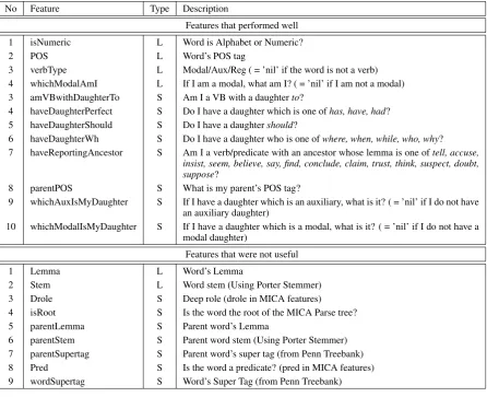
No Feature Type Description

Features that performed well 1 isNumeric L Word is Alphabet or Numeric?

2 POS L Word’s POS tag

3 verbType L Modal/Aux/Reg ( = ’nil’ if the word is not a verb) 4 whichModalAmI L If I am a modal, what am I? ( = ’nil’ if I am not a modal) 3 amVBwithDaughterTo S Am I a VB with a daughterto?

4 haveDaughterPerfect S Do I have a daughter which is one ofhas, have, had? 5 haveDaughterShould S Do I have a daughtershould?

6 haveDaughterWh S Do I have a daughter who is one ofwhere, when, while, who, why? 7 haveReportingAncestor S Am I a verb/predicate with an ancestor whose lemma is one oftell, accuse,

insist, seem, believe, say, find, conclude, claim, trust, think, suspect, doubt, suppose?

8 parentPOS S What is my parent’s POS tag?

9 whichAuxIsMyDaughter S If I have a daughter which is an auxiliary, what is it? ( = ’nil’ if I do not have an auxiliary daughter)

10 whichModalIsMyDaughter S If I have a daughter which is a modal, what is it? ( = ’nil’ if I do not have a modal daughter)

Features that were not useful

1 Lemma L Word’s Lemma

2 Stem L Word stem (Using Porter Stemmer)

3 Drole S Deep role (drole in MICA features) 4 isRoot S Is the word the root of the MICA Parse tree?

5 parentLemma S Parent word’s Lemma

6 parentStem S Parent word stem (Using Porter Stemmer) 7 parentSupertag S Parent word’s super tag (from Penn Treebank) 8 Pred S Is the word a predicate? (pred in MICA features) 9 wordSupertag S Word’s Super Tag (from Penn Treebank)

Table 1: All Features Used

a joint model, in which the heads are chosen and classified simultaneously, and a pipeline model, in which heads are chosen first and then classified. In this paper, we consider the joint model in de-tail and in Section 3.5.3, we present results of the pipeline model; they support our choice.

In the joint model, we define a four-way clas-sification task where each token is tagged as one of four classes – CB, NCB, NA, or O (nothing) – as defined in Section 2. For tagging, we ex-perimented with Support Vector Machines (SVM) and Conditional Random Fields (CRF). For SVM, we used the YAMCHA(Kudo and Matsumoto, 2000) sequence labeling system,1 _{which uses the}

TinySVM package for classification.2 _{For CRF,}

we used the linear chain CRF implementation of

1_{http://chasen.org/ taku/software/YAMCHA/} 2_{http://chasen.org/ taku/software/TinySVM/}

the MALLET(McCallum, 2002) toolkit.3

3.2 Features

We divided our features into two types - Lexi-cal and Syntactic. LexiLexi-cal features are at the to-ken level and can be extracted without any pars-ing with relatively high accuracy. We expect these features to be useful for our task. For example, isNumeric, which denotes whether the word is a number or alphabetic, is a lexical feature. Syn-tactic features of a token access its synSyn-tactic con-text in the dependency tree. For example, par-entPOS, the POS tag of the parent word in the dependency parse tree, is a syntactic feature. We used the MICA deep dependency parser (Banga-lore et al., 2009) for parsing in order to derive the syntactic features. We use MICA because we assume that the relevant information is the

predicate-argument structure of the verbs, which is explicit in the MICA output. While it is clear that having a perfect parse would yield useful fea-tures, current parsers perform at levels of accuracy lower than that of part-of-speech taggers, so that it is not a foregone conclusion that using automatic parser output helps in our task.

The list of features we used in our experiments are summarized in Table 1. The column ’Type’ denotes the type of the feature. ’L’ stands for lex-ical features and ’S’ stands for syntactic features.

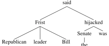
The tree below shows the dependency parse tree output by MICA for the sentenceRepublican leader Bill Frist said the Senate was hijacked.

said

Frist

Republican leader Bill

hijacked Senate

the was

In the above sentence, said and hijacked are the propositions that should be tagged. Let’s look athijackedin detail. The feature haveReportin-gAncestorofhijackedis ‘Y’ because it is a verb with a parent verb said. Similarly, the feature haveDaughterAuxwould also be ’Y’ because of daughterwas, whereaswhichAuxIsMyDaughter would get the valuewas.

We also considered several other features which did not yield good results. For example, the to-ken’s supertag (Bangalore and Joshi, 1999), the parent token’s supertag, a binary feature isRoot (Is the word the root of the parse tree?) were deemed not useful. We list the features we exper-imented with and decided to discard in Table 1.

For finding the best performing features, we did an exhaustive search on the feature space, incre-mentally pruning away features that are not use-ful.

3.3 Experiments

This section describes different experiments we conducted in detail. It explains the experimen-tal setup for both learning frameworks we used - YAMCHA and MALLET. We also explain the pipeline model in detail.

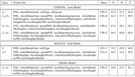
Class Description

LC Lexical features with Context

LNSN Lexical and Syntactic features with

No-context

LCSN Lexical features with Context and Syntactic

features with No-context

LCSC Lexical and Syntactic features with Context Table 2: YAMCHA Experiment Sets

3.3.1 YAMCHA Experiments

We categorized our YAMCHA experiments into different experimental conditions as shown in Table 2. For each class, we did experiments with different feature sets and (linear) context widths. Here, context width denotes the window of tokens whose features are considered. For example, a context width of 2 means that the feature vector of any given token includes, in addition to its own features, those of 2 tokens before and after it as well as the tag prediction for 2 tokens before it. ForLNSN, the context width of all features was

set to 0. ForLCSN, the context width of syntactic

features alone was set to 0. A context width of 0 for a feature means that the feature vector includes that feature of the current token only. When con-text width was non-zero, we varied it from 1 to 5, and we report the results for the optimal context width.

We tuned the SVM parameters, and the best results were obtained using the One versus All

method for multiclass classification on a quadratic kernel with acvalue of0.5. All results presented for YAMCHA here use this setting.

3.3.2 MALLET Experiments

Class Description

L Lexical features only

LS Lexical and Syntactic features Table 3: MALLET Experiment Sets

or-Class Feature Set Parm P R F YAMCHA - Joint Model

LC POS, whichModalAmI, verbType, isNumeric CW=3 61.9 52.7 56.9

LNSN POS, whichModalAmI, parentPOS, haveReportingAncestor,

whichModal-IsMyDaughter, haveDaughterPerfect, whichAuxwhichModal-IsMyDaughter, amVBwith-DaughterTo, haveDaughterWh, haveDaughterShould

CW=0 62.5 57.5 59.9

LCSN POS, whichModalAmI, parentPOS, haveReportingAncestor,

whichModalIs-MyDaughter, whichAuxIswhichModalIs-MyDaughter, haveDaughterShould CW=2 67.4 58.1 62.4

LCSC POS, whichModalAmI, parentPOS, haveReportingAncestor,

whichModal-IsMyDaughter, haveDaughterPerfect, whichAuxwhichModal-IsMyDaughter, haveDaugh-terWh, haveDaughterShould

CW=2 68.5 60.0 64.0

MALLET - Joint Model

L POS, whichModalAmI, verbType GV=1 55.1 45.0 49.6

LS POS, whichModalAmI, parentPOS, haveReportingAncestor, whichModal-IsMyDaughter, haveDaughterPerfect, whichAuxwhichModal-IsMyDaughter, haveDaugh-terWh, haveDaughterShould

GV=1 64.5 54.4 59.0

Pipeline Model

LCSC POS, whichModalAmI, parentPOS, haveReportingAncestor,

whichModal-IsMyDaughter, haveDaughterPerfect, whichAuxwhichModal-IsMyDaughter, haveDaugh-terWh, haveDaughterShould

CW=2 49.8 42.9 46.1

Table 4: Overall Results. CW = Context Width, GV = Gaussian Variance, P = Precision, R = Recall, F = F-Measure

der= “0,1”, which makes the CRF similar to Hid-den Markov Model. All results reported here use the order= “0,1”. We also conducted experiments varying the Gaussian variance parameter from 1.0 to 10.0 using the same experimental setup (i.e. we did not have a distinct tuning corpus) and ob-served that best results were obtained with a low value of 1 to 3, instead of MALLET’s default

value of10.0.

3.3.3 Pipeline Model

We also did experiments to support our choice of the joint model over the pipeline model. We chose the best performing feature configuration of the LCSC class (which is the overall best

performer as we present in Section 3.5), and set up the pipeline model. We trained a se-quence classifier using YAMCHA to identify the head tokens, where tokens are tagged as just propositional heads without distinguishing be-tween CB/NA/NCB. The predicted head tokens were then classified using a 3-Way SVM classi-fier trained on gold data.

3.4 Evaluation

For evaluation, we used 4-fold cross validation on the training data. The data was divided into 4 folds of which 3 folds were used to train a model which was tested on the 4th fold. We did this with all four configurations and all the reported results in this paper are averaged results across 4 folds. We report Recall and Precision on word tokens in our corpus for each of the three tags. It is worth noting that the majority of the words in our data will not be tagged with any of the three classes. (Recall that most words have neither of the three tags). We also report Fβ=1(F)-measure as the harmonic

mean between (P)recision and (R)ecall.

3.5 Results

This section summarizes the results of various experiments we conducted. The best perform-ing feature configuration and correspondperform-ing Pre-cision, Recall and F-measure for each experimen-tal setup discussed in previous section is presented in Table 4. The best F-measure for each category under various experimental setups is presented in Table 5.

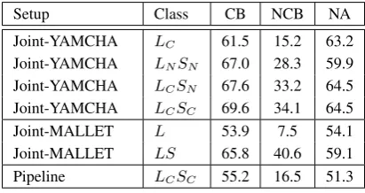
YAM-Setup Class CB NCB NA Joint-YAMCHA LC 61.5 15.2 63.2

Joint-YAMCHA LNSN 67.0 28.3 59.9

Joint-YAMCHA LCSN 67.6 33.2 64.5

Joint-YAMCHA LCSC 69.6 34.1 64.5

Joint-MALLET L 53.9 7.5 54.1

Joint-MALLET LS 65.8 40.6 59.1 Pipeline LCSC 55.2 16.5 51.3 Table 5: Results per Category (F-Measure)

CHA in a joint model. So, we first analyze this configuration in great detail in Section 3.5.1. We discuss results obtained using MALLET in Sec-tion 3.5.2 and the pipeline model in SecSec-tion-3.5.3.

3.5.1 YAMCHA - Results

As described in Section 3.3.1, we divide our experiments into 4 classes - LC, LNSN, LCSN

and LCSC. Table 4 presents the best

perform-ing feature sets and context width configuration for each class. For all experiments with context, the best result was obtained with a context width of 2, except for LC, where a context width of 3

gave the best results. The results show that syn-tactic features improve the classifier performance considerably. The best model obtained for LC

has an F-measure of 56.9%. In LNSN it

im-proves marginally to 59.9%. Adding back context to lexical features improves it to 62.4% inLCSN

whereas addition of context to syntactic features further improves this to 64.0%. We observed that the featureparentPOShas the most impact on in-creased context widths, among syntactic features. The improvement pattern of Precision and Re-call across the classes is also interesting. Syntac-tic features with no context improve Recall by 4.8 percentage points over only lexical features with context, whereas Precision improves only by 0.6 points. However, adding back context to lexical features further improves Precision by 4.9 points while Recall just improves by 0.6 points. Finally, adding context of syntactic features improves both Precision and Recall moderately. We infer that syntactic features (without context) help identify more annotatable patterns thereby improving Re-call, whereas linear context helps removing the wrong ones, thereby improving Precision.

The per-category F-measure results presented in Table 5 are also interesting. The CB F-measure improves by 8.1 points and NCB improves 18.9 points fromLC toLCSC. But, the improvement

in NA F-measure is only a marginal 1.3 points between LC and LCSC. Furthermore, the

F-measure decreases by 3.3 points when syntactic and lexical features with no context are used. On analysis, we found that NAs often occur in syn-tactic structures likewant to findorshould go (de-onticshould), in which the relevant words occur in a small linear window. In contrast, NCBs are often signaled by deeper syntactic structures. For example, in He said that his visit to the US will mainly focus on the humanitarian issues, a simpli-fied sentence from our training set, the verbfocus

is an NCB because it is in the scope of the report-ing verbsaid(specifically, it is its daughter). This could not be captured using the context because

saidandfocusare far apart in the sentence. But a correct parse tree givesfocusas the daughter of

said. So, a feature likehaveReportingAncestor could easily capture this. It is also the case that the root of a dependency parse tree would mostly be a CB. This is captured by the featureparentPOS having value ‘nil’. This property also cannot be captured by lexical features alone.

However, NCB performs much worse than the other two categories. NCB is a class which occurs rarely compared to CB and NA in our corpus. Out of the1,357propositions tagged, only176were

NCB. We assume that this could be a main factor of its poor performance.

We analyzed the performance across the folds. Fold-2 contains only 0.03% NCBs compared to 1.89% on the rest of the folds. Similarly, it con-tains 6.43% NAs compared to 3.82% across other folds. However, our best performing model gives a Recall of 59.1% with a Precision of 69.7% (F-measure 64.0%) for Fold-2, which is as good as other folds. Hence, we observe that our learned model is robust under distributional variations.

3.5.2 MALLET Results

As explained in Section 3.3.2, we explored MALLET-CRF using two experimental condi-tions L and LS. Table 4 presents the best

re-sults again show that syntactic features improve the classifier performance considerably. The best model obtained for L class has an F-measure of 49.6%, whereas addition of syntactic features im-proves this to 59.0%. Both Precision and Recall are improved by 9.4 percentage points as well.

However, MALLET-CRF’s performance was comparatively worse than YAMCHA’s SVM. The best model for MALLET (LS) obtained an

F-measure of 59.0% which is 5.0 percentage points less than that of the best model for YAMCHA (LCSC).

It is interesting to note that MALLET per-formed well on predicting NCB. The highest NCB F-measure of MALLET - 40.6% is 6.5 percent-age points higher than the highest NCB F-measure for YAMCHA. However, corresponding CB and NA F-measures were 61.2% and 56.1% which are much lower than YAMCHA’s performance for these categories.

Also, MALLET was more time efficient than YAMCHA. On an average, for our corpus size and feature sets, MALLET ran 3 times as fast as YAMCHA in a cross validation setup (i.e. training and testing together).

3.5.3 Joint Model vs Pipeline Model

As discussed in Section 3.3.3, we set up a pipeline model for the best performing configu-ration ofLCSC class of YAMCHA experiments.

The head prediction step of the pipeline obtained an F-measure of 83.9% with Precision and Re-call of 86.7% and 81.2%, respectively, across all 4 folds. The 3-way classification step to classify the belief of the identified head obtained an ac-curacy of 72.7% across all folds. In the pipeline model, false positives and false negatives adds up from step 1 and step 2, where as only the true positives of step 2 is considered as the true pos-itives overall. In this way, the overall Precision was only 49.8% and Recall was 42.9% with an F-measure of 46.1% as shown in Table 4. The results for CB/NCB/NA separately are given in Table 5. The per-category best F-measure was decreased by 14.4, 17.6 and 13.2 percentage points from the YAMCHA joint model for CB, NCB and NA, re-spectively. The performance gap is big enough to conclude that our choice of joint model was right.

4 Related Work

Our work falls in the rich tradition of modeling agents in terms of their cognitive states (for ex-ample, (Rao and Georgeff, 1991)) and relating this modeling to language use through extensions to speech act theory (for example, (Perrault and Allen, 1980; Clark, 1996; Bunt, 2000)). These no-tions have been particularly fruitful in the dialog community, where dialog act tagging is a major topic of research; to cite just one prominent ex-ample: (Stolcke et al., 2000). A dialog act repre-sents the communicative intention of the speaker, and its recognition is crucial for the building of dialog systems. The specific contribution of this paper is to investigate exactly how discourse par-ticipants signal their beliefs using language, and the strength of their beliefs; this latter point is not usually included in dialog act tagging.

This paper is not concerned with issues relating to logics for belief representation or inferencing that can be done on beliefs (for an overview, see (McArthur, 1988)), nor theories of automatic be-lief ascription (Wilks and Ballim, 1987). For ex-ample, this paper is not concerned with determin-ing whether a belief in the requirement ofpentails

the belief inp; instead, we are only interested in

whether the writer wants the reader to understand whether the writer holds a belief in the require-ment thatpor inpdirectly. This paper is also not

concerned with subjectivity (Wiebe et al., 2004), the nature of the proposition p (statement about

interior world or external world) is not of interest, only whether the writer wants the reader to believe the writer believesp. This paper is also not

con-cerned with opinion and determining the polarity (or strength) of opinion (for example: (Somasun-daran et al., 2008)), which corresponds to the de-sire dimension. Thus, this work is orthogonal to the extensive literature on opinion classification.

is more limited in several ways: we currently only model the writer’s beliefs; we do not express po-larity (we believe we can derive it from the syn-tax and lexicon); Saur´ı and Pustejovsky (2008) ask their annotators to perform extensive linguis-tic transformations on the text to obtain a “nor-malized” representation of propositional content (we simply ask the annotators to make a judg-ment about the writer’s strength of belief with respect to a given proposition, and expect to be able to extract representations of pure proposi-tional meaning independently); and finally, Saur´ı and Pustejovsky (2008) have a more fine-grained representation of non-committed belief. While it is plausible to distinguish between more or less firm non-committed belief, we believe the crucial distinction is between committed belief and non-committed belief. Furthermore, Saur´ı and Puste-jovsky (2008) group reported speech with non-belief statements (our NA), while we group them with weak belief (our NCB). The reason for our decision is that we wanted to keep NA as a cat-egory which contains no-one’s beliefs, as we as-sumed this is semantically more coherent. The category NCB thus covers beliefs which the writer does not hold firmly or has expressed no opinion on — which is different from propositions which the writer has clearly attributed to other cognitive states (such as desire). In principle, we believe a 4-way distinction is the right approach, but our NCB category is already the least frequent, and splitting it would have resulted in two very rare classes. Another difference include the use of the word “fact” in the FactBank manual, which we avoid because we are interested in cognitive mod-eling; however, this is merely a terminological is-sue.

Other related works explored belief systems in an inference scenario as opposed to an intentional-ity scenario. In work by (Krestel et al., 2008), the authors explore belief in the context of reported speech in news media: they track newspaper text looking for elements indicating evidentiality. This is different from our work, since we seek to make explicit the intention of the author or the speaker.

5 Future Work

We are exploring ways to utilize the FactBank an-notated corpus for our purpose, with the goal of automatically converting it to our annotation for-mat. With the added data from FactBank, we hope to be able to split the NCB category into WB (weak belief) and RS (reported speech). We will also explore learning embedded belief attri-butions, as annotated in FactBank.

We found that the per-sentence F-measure has a small positive correlation with the length-normalized probability of the MICA derivation (a measure of parse confidence). In case of a bad parse, syntax features add noise which in turn re-duces classifier performance. We are planning to exploit this correlation in order to choose sen-tences for selective self-training. Another direc-tion we are looking to extend this work is to em-ploy active learning to overcome the shortcom-ings of a small training set. Also, we found fre-quent use of epistemic and deontic modals in our data. Both types of modals have identical syntac-tic structure, but they receive very different anno-tations. This is not easily captured in our system. We are exploring ways to handle this.

We will release our Committed Belief Tagging tool as a standalone black-box tool. We also in-tend to release the annotated corpus.

6 Acknowledgments

This work is supported, in part, by the Johns Hop-kins Human Language Technology Center of Ex-cellence. Any opinions, findings, and conclusions or recommendations expressed in this material are those of the authors and do not necessarily reflect the views of the sponsor. We thank Bonnie Dorr, Lori Levin and our other partners on the TTO8 project. We also thank several anonymous review-ers for their constructive feedback.

References

Bangalore, Srinivas and Aravind Joshi. 1999. Su-pertagging: An approach to almost parsing. Com-putational Linguistics, 25(2):237–266.

A probabilistic dependency parser based on tree in-sertion grammars. InNAACL HLT 2009 (Short Pa-pers).

Bratman, Michael E. 1999 [1987]. Intention, Plans, and Practical Reason. CSLI Publications.

Bunt, Harry. 2000. Dialogue pragmatics and context specification. In Bunt, Harry and William J. Black, editors,Abduction, Belief and Context in Dialogue, pages 81–150.

Clark, Herbert H. 1996. Using Language. cup, Cam-bridge, England.

Cohen, Philip R. and Hector J. Levesque. 1990. Ratio-nal interaction as the basis for communication. In Philip Cohen, Jerry Morgan and James Allen, edi-tors,Intentions in Communication. MIT Press.

Diab, Mona T., Lori Levin, Teruko Mitamura, Owen Rambow, Vinodkumar Prabhakaran, and Weiwei Guo. 2009. Committed belief annotation and tag-ging. In ACL-IJCNLP ’09: Proceedings of the Third Linguistic Annotation Workshop, pages 68– 73, Morristown, NJ, USA. Association for Compu-tational Linguistics.

Grice, Herbert Paul. 1975. Logic and conversation. In Cole, P. and J. Morgan, editors,Syntax and seman-tics, vol 3. Academic Press, New York.

Hovy, Eduard H. 1993. Automated discourse gener-ation using discourse structure relgener-ations. Artificial Intelligence, 63:341–385.

Krestel, Ralf, Sabine Bergler, and Ren´e Witte. 2008. Minding the Source: Automatic Tagging of Re-ported Speech in Newspaper Articles. In (ELRA), European Language Resources Association, edi-tor, Proceedings of the Sixth International Lan-guage Resources and Evaluation (LREC 2008), Marrakech, Morocco, May 28–30.

Kudo, Taku and Yuji Matsumoto. 2000. Use of sup-port vector learning for chunk identification. In Proceedings of CoNLL-2000 and LLL-2000, pages 142–144.

Mann, William C. and Sandra A. Thompson. 1987. Rhetorical Structure Theory: A theory of text orga-nization. Technical Report ISI/RS-87-190, ISI.

McArthur, Gregory L. 1988. Reasoning about knowl-edge and belief: a survey. Computational Intelli-gence, 4:223–243.

McCallum, Andrew Kachites. 2002. Mal-let: A machine learning for language toolkit. http://mallet.cs.umass.edu.

Moore, Johanna. 1994. Participating in Explanatory Dialogues. MIT Press.

Perrault, C. Raymond and James F. Allen. 1980. A plan-based analysis of indirect speech acts. Compu-tational Linguistics, 6(3–4):167–182.

Rao, Anand S. and Michael P. Georgeff. 1991. Mod-eling rational agents within a BDI-architecture. In Allen, James, Richard Fikes, and Erik Sandewall, editors, Proceedings of the 2nd International Con-ference on Principles of Knowledge Representation and Reasoning, pages 473–484. Morgan Kaufmann publishers Inc.: San Mateo, CA, USA.

Saur´ı, Roser and James Pustejovsky. 2007. Determin-ing Modality and Factuality for Textual Entailment. InFirst IEEE International Conference on Semantic Computing., Irvine, California.

Saur´ı, Roser and James Pustejovsky. 2008. From Structure to Interpretation: A Double-layered An-notation for Event Factuality. InProceedings of the 2nd Linguistic Annotation Workshop. LREC 2008.

Somasundaran, Swapna, Janyce Wiebe, and Josef Rup-penhofer. 2008. Discourse level opinion interpre-tation. In Proceedings of the 22nd International Conference on Computational Linguistics (Coling 2008), pages 801–808, Manchester, UK, August. Coling 2008 Organizing Committee.

Stolcke, Andreas, Klaus Ries, Noah Coccaro, Eliza-beth Shriberg, Rebecca Bates, Daniel Jurafsky, Paul Taylor, Rachel Martin, Carol Van Ess-Dykema, and Marie Meteer. 2000. Dialogue act modeling for automatic tagging and recognition of conversational speech. Computational Linguistics, 26:339–373. Stone, Matthew. 2004. Intention, interpretation and

the computational structure of language. Cognitive Science, 24:781–809.

Wiebe, Janyce, Theresa Wilson, Rebecca Bruce, Matthew Bell, and Melanie Martin. 2004. Learning subjective language. InComputational Linguistics, Volume 30 (3).