Imbalanced Classification Using Dictionary based Prototypes and Hierarchical Decision Rules for Entity Sense Disambiguation

Imbalanced Classification Using Dictionary-based Prototypes and

Hierarchical Decision Rules for Entity Sense Disambiguation

Tingting Mu

National Centre for Text Mining University of Manchester

[email protected]

Xinglong Wang

National Centre for Text Mining University of Manchester

[email protected]

Jun’ichi Tsujii

Department of Computer Science University of Tokyo

[email protected]

Sophia Ananiadou National Centre for Text Mining

University of Manchester

[email protected]

Abstract

Entity sense disambiguation becomes dif-ficult with few or even zero training in-stances available, which is known as im-balanced learning problem in machine learning. To overcome the problem, we create a new set of reliable training in-stances from dictionary, called dictionary-based prototypes. A hierarchical classifi-cation system with a tree-like structure is designed to learn from both the prototypes and training instances, and three different types of classifiers are employed. In addi-tion, supervised dimensionality reduction is conducted in a similarity-based space. Experimental results show our system out-performs three baseline systems by at least 8.3%as measured by macroF1score.

1 Introduction

Ambiguities in terms and named entities are a challenge for automatic information extraction (IE) systems. The problem is particularly acute for IE systems targeting the biomedical domain, where unambigiously identifying terms is of fun-damental importance. In biomedical text, a term (or its abbreviation (Okazaki et al., 2010)) may belong to a wide variety of semantic categories (e.g., gene, disease, etc.). For example, ERmay denote protein estrogen receptor in one context, but cell subunitendoplasmic reticulumin another,

not to mention it can also mean emergency room. In addition, same terms (e.g., protein) may be-long to many model organisms, due to the nomen-clature of gene and gene products, where genes in model organisms other than human are given, whenever possible, the same names as their hu-man orthologs (Wain et al., 2002). On the other hand, public biological databases keep species-specific records for the same protein or gene, making species disambiguation an inevitable step for assigning unique database identifiers to entity names in text (Hakenberg et al., 2008; Krallinger et al., 2008).

and you have to select a sample, or (ii) you have no data at all and you have to go through an

in-volved process to create them” (Provost, 2000).

Given an entity disambiguation task with imbal-anced data, this paper explores how to create more informative training instances for minority classes and how to improve the large-scale training for majority classes.

Previous research has shown that words denot-ing class information in the surrounddenot-ing context of an entity can be an informative indicator for dis-ambiguation (Krallinger et al., 2008; Wang et al., 2010). Such words are refered to as “cue words” throughout this paper. For example, to disam-biguate the type of an entity, that is, whether it is a protein, gene, or RNA, looking at words such

asprotein,geneandRNAare very helpful

(Hatzi-vassiloglou et al., 2001). Similarly, for the task of species disambiguation (Wang et al., 2010), the occurrence of mouse p53 strongly suggests

thatp53is a mouseprotein. In many cases, cue

words are readily available in dictionaries. Thus, for the minority classes, instead of creating arti-ficial training instances by commonly used sam-pling methods (Haibo and Garcia, 2009), we pro-pose to create a new set of real training instances by modelling cue words from a dictionary, called dictionary-based prototypes. To learn from both the original training instances and the dictionary-based prototypes, a hierarchical classification sys-tem with a tree-like structure is designed. Further-more, to cope with the large number of features representing each instance, supervised orthogo-nal locality preserving projection (SOLPP) is con-ducted for dimensionality reduction, by simulta-neously preserving the intrinsic structures con-structed from both the features and labels. A new set of lower-dimensional embeddings with better discriminating power is obtained and used as in-put to the classifier. To cope with the large num-ber of training instances in some majority classes, we propose a committee machine scheme to ac-celerate training speed without sacrificing classi-fication accuracy. The proposed method is evalu-ated on a species disambiguation task, and the em-pirical results are encouraging, showing at least 8.3% improvement over three different baseline systems.

2 Related Work

Construction of a classification model using su-pervised learning algorithms is popular for entity disambiguation. A number of researchers have tackled entity disambiguation in general text us-ing wikipedia as a resource to learn classifica-tion models (Bunescu and Pas¸ca, 2006). Hatzi-vassiloglou et al. (2001) studied disambiguating proteins, genes, and RNA in text by training var-ious classifiers using entities with class informa-tion provided by adjacent cue words. Wang et al. (2010) proposed a “hybird” system for species disambiguation, which heuristically combines re-sults obtained from classifying the context, and those from modeling relations between cue words and entities. Although satisfactory performance was reported, their system incurs higher computa-tional cost due to syntactic parsing and the binary relation classifier.

Many imbalanced learning techniques, as re-viewed by Haibo and Garcia (2009), can also be used to achieve the same purpose. However, to our knowledge, there is little research in apply-ing these machine learnapply-ing (ML) techniques to en-tity disambiguation. It is worth mentioning that although these ML techniques can improve the learning performance to some extent, they only consider the information contained in the origi-nal training instances. The created instances do not add new information, but instead utilize the original training information in a more sophisti-cated way. This motivates us to pursue a differ-ent method of creating new training instances by using information from a related and easily ob-tained source (e.g., a dictionary), similar to trans-fer learning (Pan and Yang, 2009).

3 Task and Corpus

en-tities are annotated, we assign a species identi-fier to every entity mention. The types of entities studied in this work are genes and gene products (e.g., proteins), and we use the NCBI Taxonomy1

(taxon) IDs as species tags and to build the proto-types. Note that this paper focuses on the task of species disambiguation and makes the assumption that the named entities are already recognised.

Consider the following sentence as an exam-ple: if one searches the proteins (i.e., the under-lined term) in a protein database, he/she will find they belong to many model organisms. However, in this particular context, CD200R-CD4d3+4 is

human and mouse protein, while rCD4d3+4 is

a rat one.2 _{We call such a task of assigning}

species identifiers to entities, according to context, as species disambiguation.

The amounts of human and mouse

CD200R-CD4d3+4 and rCD4d3+4 protein on the microarray spots were similar as visualized by the red fluo-rescence of OX68 mAb recognising the CD4 tag present in each of the recombinant proteins.

The informative cue words (e.g., mouse) used to help species disambiguation are called species words. In this work, species words are defined as any word that indicates a model organism and also appears in the organism dictionaries we use. They may have various parts-of-speech, and may also contain multiple tokens (despite the name species

word). For example, “human”, “mice”, “bovine” and “E. Coli” are all species words. We detect these words by automatic dictionary lookup: a word is annotated as a species word if it matches an entry in a list of organism names. Each entry in the list contains a species word and its correspond-ing taxon ID, and the list is merged from two dic-tionaries: the NCBI Taxonomy and the UniProt controlled vocabulary of species.3_{The NCBI}

por-tion is a flattened NCBI Taxonomy (i.e., without hierarchy) including only the identifiers ofgenus

andspecies ranks. In total, the merged list

con-1_{http://www.ncbi.nlm.nih.gov/sites/entrez?db=}

taxon-omy

2_{Prefix ‘r’ in “rCD4d3+4” indicates that it is aratprotein.} 3_{http://www.expasy.ch/cgi-bin/speclist}

tains 356,387 unique species words and 272,991 unique species IDs. The ambiguity in species words is low:3.86%of species words map to mul-tiple IDs, and on average each word maps to1.043 IDs.

The proposed method was evaluated on the corpus developed in (Wang et al., 2010), con-taining 6,223 genes and gene products, each of which was manually assigned with either a taxon ID or an “Other” tag, with human being the most frequent at 50.30%. With the extracted features and the species ID tagged by domain experts, each occurrence of named entities can be represented as a d-dimensional vector with a label. Species disambiguation can be mod-elled as a multi-classification task: Givenn train-ing instances {x_i}n_i=1, their n _×d feature ma-trix X = [xij] and n-dimensional label vector

y = [y1, y2, . . . , yn]T are used to train a

clas-sifierC(_·), wherexi = [xi1, xi2, . . . , xid]T,yi ∈ {1,2, . . . , c_}, and c denotes the number of ex-isting species in total. Given m different query instances {xˆ_i}m_i=1, their m _× d feature matrix ˆ

X = [ˆxij] are used as the input to the trained

classifier, so that their labels can be predicted by

{C( ˆxi)}mi=1.

4 Proposed Method

4.1 Dictionary-based Prototypes

For each existing species, we create a b -dimensional binary vector, given as pi =

[pi1, pi2, . . . , pib]T, using b different species

words listed in the dictionary as features, which is called dictionary-based prototype. The binary value pij denotes whether the jth species word

belongs to theith species in the dictionary. This leads to a c×b feature matrix P = [pij] for c

species.

Considering that the species words preceding and appearing in the same sentence as an en-tity can be informative indicators for the possible species of this entity, we create two morem×b bi-nary feature matrices for the query instances with the samebspecies words as features:X1ˆ = [ˆx(1)_ij ] and_X2ˆ _{= [ˆx}(2)

ij ], wherexˆ

(1)

ij denotes whether the

jth species word is the preceding word of theith entity, and xˆ(2)_ij denotes whether the jth species word appears in the same sentence as theith en-tity but is not preceding word. Thus, the similar-ity between each query entsimilar-ity and existing species can be simply evaluated by calculating the inner-product between the entity instance and the cor-responding prototype. This leads to the following m_×csimilarity matrixSˆ= [ˆsij]:

ˆ

S=θX1ˆ PT + (1−θ) ˆX2PT, (1)

where0≤θ≤1is a user-defined parameter con-trolling the degree of indicating reliability of the preceding word and the same-sentence word. The n×csimilarity matrixS= [sij]between the

train-ing instances and the species can be constructed in exactly the same way. Based on empirical expe-rience, the preceding word indicates the entity’s species more accurately than the same-sentence word. Thus, θ is preferred to be set as greater than 0.5. The obtained similarity matrix will be used in the nearest neighbour classifier (see Sec-tion 4.2.1).

Both the original training instances Xand the newly created prototypes Pare used to train the proposed hierarchical classification system. Sub-ject to the nature of the classifier employed, it is convenient to construct one single feature matrix

Nearest Neighbor Classifier

(IT1)

Minority Classes

Majority Classes

SOLPP-FLDA Classifier

(IT2)

Small-scale Majority

Classes

Large-scale Majority

Classes

Committee Classifier

(END)

Yes

No Yes

No

Output: Instances with predicted labels belonging to MI

Output: Instances with predicted labels belonging to SMA

Output: Instances with predicted labels belonging to LMA

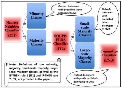
Note: Definition of the minority, majority, small-scale majority, large-scale majority classes, as well as the IF-THEN rule 1 (IT1) and IF-THEN rule 2 (IT2) are provided in the paper.

Figure 1: Structure of the proposed hierarchical classification system

instead of usingXandPindividually. Aiming at keeping the same similarity values between each entity instance and the species prototype, we con-struct the following(n+c)×(d+b)feature matrix for both the training instances and prototypes:

F=

X θX1+ (1−θ)X2

0 P

, (2)

whereX1andX2are constructed in the same way as_X1ˆ _andX2ˆ _{but for training instances. Their} cor-responding label vector isl= [yT,1,2, . . . , c]T.

4.2 Hierarchical Classification

Multi-stage or hierarchical classification (Giusti et al., 2002; Podolak, 2007; Kurzy´nski, 1988) is widely used in many complex multi-category classification tasks. Existing research shows such techniques can potentially achieve right trade-off between accuracy and resource allocation (Giusti et al., 2002; Podolak, 2007). Our proposed hier-archical system has a tree-like structure with three different types of classifier at nodes (see Figure 1). Different classes are organized in a hierarchical order to be classified based on the corresponding numbers of available training instances. Letting ni denote the number of training instances

avail-able in theithe class excluding the created proto-types, we categorize the classes as follows:

• Minority Classes (MI): Classes with less training instances than the threshold: MI =

{i: ni

• Majority Classes (MA):Classes with more training instances than the threshold: MA=

{i: ni

n ≥σ1, i∈ {1,2. . . , c}}.

• Small-scale Majority Classes (SMA):

Ma-jority Classes with less training instances than the threshold: SMA = {i : ni

n <

σ2, i∈MA}.

• Large-scale Majority Classes (LMA): Ma-jority Classes with more training instances than the threshold: LMA = {i : ni

n ≥

σ2, i∈MA}.

Here, 0 < σ1 < 1 and 0 < σ2 < 1 are size thresholds set by users. We have MI∩MA = ∅, SMA∩LMA=_∅, and SMA_∪LMA=MA.

The tree-like hierarchical structure of our sys-tem is determined by MI, MA, SMA, and LMA. We propose two IF-THEN rules to control the sys-tem: Given a query instancexˆi, the level 1

clas-sifierC1 is used to predict whetherxˆi belongs to

MA or a specific class in MI, which wer call IF-THEN rule 1 (IT1). Ifxˆibelongs to MA, the level

2 classifier C2 is used to predict whether xˆi

be-longs to LMA or a specific class in SMA, called IF-THEN rule 2 (IT2). Ifxˆibelongs to LMA, the

level 3 classifier C3 finally predicts the specific class in LMA xˆi belongs to. We explain in the

following sections how the classifiersC1,C2, and C3work in detail.

4.2.1 Nearest Neighbour Classifier

The goal of the nearest neighbour classifier, de-noted by C1, is to decide whether the nearest-neighbour prototype of the query instance be-longs to MI. The only used training instances are our created dictionary-based prototypes {p_i}c

i=1 with the label vector[1,2, . . . , c]T. The nearest-neighbour prototype of the query instancexˆi

pos-sesses the maximum similarity toxˆi:

N N( ˆxi) = arg max

j=1,2, ..., csˆij, (3)

wheresˆij is obtained by Eq. (1). Consequently,

the output of the classifierC1is given as

C1( ˆxi) =

N N( ˆxi), IfN N( ˆxi)∈MI,

0, Otherwise.

(4)

The IF-THEN rule 1 can then be expressed as

Action(IT1)₌

Go toC2, IfC1( ˆxi) = 0,

Stop, Otherwise.

4.2.2 SOLPP-FLDA Classifier

The goal of the SOLPP-FLDA classifier, de-noted byC2, is to predict whether the query in-stance belongs to LMA or a specific class in SMA. In this classifier, the used training instances are the original training entities and the dictionary-based prototypes, both belonging to MA. The fea-ture matrixFand the label vectorldefined in Sec-tion 4.1 are used, but with instances from MI re-moved (we usen˜to denote the number of remain-ing trainremain-ing instances, and the same symbolFfor feature matrix). The used label vector_l˜_{to trainC}

2 should be re-defined as˜_{li =liifli ∈SMA, and 0} otherwise.

First, we propose to implement orthog-onal locality preserving projection (OLPP) (Kokiopoulou and Saad, 2007) in a supervised manner, leading to SOLPP, to obtain a smaller set of more powerful features for classification. Also, we conduct SOLPP in a similarity-based feature space computed from (d+ 2b) original features by employing dot-product based similarity, given by FFT_{. As explained later, to compute the}

new features from FFT _{instead of the original}

features F achieves reduced computational cost. Ann˜_×kprojection matrixV= [vij]is optimized

in this n-dimensional similarity-based feature space. The optimal projections are obtained by minimizing the weighted distances between the lower-dimensional embeddings so that “similar” instances are mapped together in the projected feature space. Mathematically, this leads to the following constrained optimization problem:

min

V∈Rn˜×k_, VT_V=I

k×k

tr[VT_FT_F(D−W)FFT_{V], (5)}

whereW = [wij]denotes the n×nweight

ma-trix withwijdefining the degree of “closeness” or

“similarity” between theith andjth instances,D is a diagonal matrix with{di =P_jn˜₌₁wij}˜ni=1as the diagonal elements.

data, e.g. for OLPP. One common way to define the adjacency is by including the K-nearest neigh-bors (KNN) of a given node to its adjacency list, which is also called the KNN-graph (Kokiopoulou and Saad, 2007). There are two common ways to define the weight matrix: constant value, where wij = 1if the ith andjth samples are adjacent,

while wij = 0 otherwise, and Gaussian kernel.

We will denote in the rest of the paper such a weight matrix computed only from the features as WX. Ideally, if the features can accurately

describe all the discriminating characteristics, the samples that are close or similar enough to each other should have the same label vectors. How-ever, when processing real dataset, what may hap-pen is that, in the d-dimensional feature space, the data points that are close to each other may belong to different categories, while on the con-trary, the data points that are in a distant to each other may belong to the same category. In thek -dimensional projected feature space obtained by OLPP, one may have the same problem. Because OLPP solves the constrained optimization prob-lem in Eq. (5) using WX: if two instances are

close or similar to each other in the original fea-ture space, they will be the same close or simi-lar to each other in the projected space. To solve this problem, we decide to modify the “closeness” or “similarity” between instances in the projected feature space by considering the label informa-tion. The following computation of a supervised weight matrix is used for our SOLPP:

W= (1−α)WX +αLLT, (6)

where 0 _≤ α _≤ 1 is a user-defined parameter controlling the tradeoff between the label-based and feature-based neighborhood structures, and L = [lij] is an n˜ × c binary label matrix with

lij = 1if theith instance belongs to thejth class,

andlij = 0otherwise.

The optimal solution of Eq. (5) is the top (k + 1)th eigenvectors of the n˜ _×n˜ symmetric matrix FT_{F(D− W)FF}T_{, corresponding to the}

k+ 1smallest eigenvalues, but with the top one eigenvector removed, denoted byV∗_{. It is worth}

to mention that if the original feature matrix Fis used as the input of SOLPP, one needs to com-pute the eigen-decomposition of the (d+b) _×

(d+b)symmetric matrixFT(D−W)F. The cor-responding computation complexity increases in O((d+b)3_{), which is unacceptable in practical} whend+b n˜. The projected features for the training instances are computed by

Z=FFTV∗. (7)

Given a different set ofmquery instances with an m_×(d+b)feature matrix,

ˆ

F= [ ˆX, θX1ˆ + (1₋θ) ˆX2], (8)

their embeddings can be easily obtained by

ˆ

Z= ˆFFˆTV∗. (9)

Then, the projected feature matrix Z and label vector˜_{l are used to train a multi-class classifier.} By employing the one-against-all scheme, differ-ent binary classifiers {C(2)_{i }i∈SMA∪{0}} with label space {+1,₋1_} are trained. For the ith class (i∈SMA∪{0}), the training instances belonging to it are labeled as positive, otherwise negative. In each binary classifierC(2)_i , a separating function

f_i(2)(x) =xTw(2)_i +b(2)_i (10)

is constructed, of which the optimal values of the weight vectorw_i(2)and biasb(2)_i are computed us-ing Fisher’s linear discriminant analysis (FLDA) (Fisher, 1936; Mu, 2008). Finally, the output of the classifierC2 can be obtained by assigning the most confident class label to the query instancexˆi,

with the confidence value indicated by the value of separating function:

C2( ˆxi) = arg max j∈SMA∪{0}f

(2)

j ( ˆxi). (11)

The IF-THEN rule 2 can then be expressed as

Action(IT2)₌

Go toC3, IfC2( ˆxi) = 0,

Stop, Otherwise.

4.2.3 Committee Classifier

instances are entities and dictionary-based proto-types only belonging to LMA. With the same one-against-all scheme, there are large number of pos-itive and negative training instances to train a bi-nary classifier for a class in LMA. To accelerate the training procedure without sacrificing the ac-curacy, the following scheme is designed.

Letting ne denote the number of experts in

committee, all the training instances are averagely divided intone+ 1groups each containing similar

numbers of training instances from the same class. The instances in theith and the(i+1)th groups are used to train theith expert classifier. This achieves overlapped training instances between expert clas-sifiers. The output value ofC(3)_i is not the class in-dex as used inC2, but the value of the separating function of the most confident class, denoted by f_i(3). Different from the commonly used majority voting rule, we only trust the most confident ex-pert. Thus, the output of C3 for a query instance

ˆ

xican be obtained by

C3( ˆxi) = arg max j=1,2, ..., ne

f_j(3)( ˆxi). (12)

By using C3, different expert classifiers can be trained in parallel. The total training time is equal to that of the slowest expert classifier. The more expert classifiers are used, the faster the system is, however, the less accurate the system may become due to the decrease of used training instances for each expert, especially the positive instances in the case of imbalanced classification. This is also the reason we do not apply the committee scheme to SMA classes.

5 Experiments

5.1 System Evaluation and Baseline

We evaluate the proposed method using 5-fold cross validation, with around 4,980 instances for training, and 1,245 instances for test in each trial. We compute the F1 score for each species, and employ macro- and micro- average scheme to compute performance for all species. Three base-lines for comparison include:

• Baseline 1 (B1) : A maximum entropy

model trained with training data only.

• Baseline 1 (B2) : Combination of B1 and the species dictionary using rules employed in Wang et al. (2010).

• Baseline 2 (B3): The “hybrid” system com-bining B1, the dictionary and a relation model4_{using rules (Wang et al., 2010).}

Our hierarchical classification system were imple-mented in two ways:

• HC: Only the training data on its own is used to train the system.

• HC/D: Both the training data and the

dictionary-based prototypes are used to train the system.

5.2 Results and Analysis

The proposed system was implemented withθ = 0.8,α= 0.8,ne= 4, andk= 1000. The species

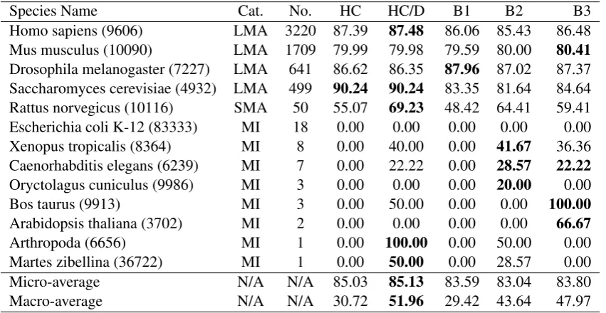
9606, 10090, 7227, and 4932 were categorized as LMA, the species 10116 as SMA, and the rest sep-cies as MI. To compute the supervised weight ma-trix, the percentage of the used KNN in the KNN-graph was 0.6. Parameters were not fine tuned, but set based on our empirical experience on previous classification research. As shown in Table 1: HC and B1 were trained with the same instances and features, and HC outperformed B1 in both macro and micro F1. Both HC and B1 obtained zeroF1 scores for most minority species, showing that it is nearly impossible to correctly label the query in-stances of minority classes, due to lack of training data. By learning from a related resource, HC/D, B2, and B3 yielded better macro performance. In particular, while HC/D and B2 learned from the same dictionary and training data, HC/D outper-formed B2 by 19.1%in macro and 2.5% in mi-cro F1. B3 aimed at improving the mami-cro perfor-mance by employing computationally expensive syntactic parsers and also by training an extra re-lation classifier. With the same goal, HC/D inte-grated the cue word information into the ML clas-sifier in a more general way, and yielded an8.3% improvement over B3, as measured by macro-F1.

4_{This is an SVM model predicting relations between}

Species Name Cat. No. HC HC/D B1 B2 B3 Homo sapiens (9606) LMA 3220 87.39 87.48 86.06 85.43 86.48 Mus musculus (10090) LMA 1709 79.99 79.98 79.59 80.00 80.41 Drosophila melanogaster (7227) LMA 641 86.62 86.35 87.96 87.02 87.37 Saccharomyces cerevisiae (4932) LMA 499 90.24 90.24 83.35 81.64 84.64 Rattus norvegicus (10116) SMA 50 55.07 69.23 48.42 64.41 59.41 Escherichia coli K-12 (83333) MI 18 0.00 0.00 0.00 0.00 0.00 Xenopus tropicalis (8364) MI 8 0.00 40.00 0.00 41.67 36.36 Caenorhabditis elegans (6239) MI 7 0.00 22.22 0.00 28.57 22.22 Oryctolagus cuniculus (9986) MI 3 0.00 0.00 0.00 20.00 0.00

Bos taurus (9913) MI 3 0.00 50.00 0.00 0.00 100.00

Arabidopsis thaliana (3702) MI 2 0.00 0.00 0.00 0.00 66.67

Arthropoda (6656) MI 1 0.00 100.00 0.00 50.00 0.00

Martes zibellina (36722) MI 1 0.00 50.00 0.00 28.57 0.00

Micro-average N/A N/A 85.03 85.13 83.59 83.04 83.80

Macro-average N/A N/A 30.72 51.96 29.42 43.64 47.97

Table 1: Performance is compared in F1 (%), where “No.” denotes the number of training instances and “Cat.” denotes the category of species class as defined in Section 4.2.

6 Conclusions and Future Work

Disambiguating bio-entities presents a challenge for traditional supervised learning methods, due to the high number of semantic classes and lack of training instances for some classes. We have pro-posed a hierarchical framework for imbalanced learning, and evaluated it on the species disam-biguation task. Our method automatically builds training instances for the minority or missing classes from a cue word dictionary, under the as-sumption that cue words in the surrounding con-text of an entity strongly indicate its semantic cat-egory. Compared with previous work (Wang et al., 2010; Hatzivassiloglou et al., 2001), our method provides a more general way to integrate the cue word information into a ML framework without using deep linguistic information.

Although the species disambiguation task is specific to bio-text, the difficulties caused by im-balanced frequency of different senses are com-mon in real application of sense disambiguation. The proposed technique can also be applied to other domains, providing the availability of a cue word dictionary that encodes semantic informa-tion regarding the target semantic classes. Build-ing such a dictionary from scratch can be chal-lenging, but may be easier compared to manual

annotation. In addition, such dictionaries may al-ready exist in specialised domains.

Acknowledgment

The authors would like to thank the biologists who annotated the species corpus, and National Cen-tre for Text Mining. Funding: Pfizer Ltd.; Joint Information Systems Committee (to UK National Centre for Text Mining)

References

Agirre, E. and D. Martinez. 2004. Unsupervised WSD based on automatically retrieved examples: The im-portance of bias. InProceedings of EMNLP. Bunescu, R. and M. Pas¸ca. 2006. Using

encyclope-dic knowledge for named entity disambiguation. In

Proceedings of EACL.

Fisher, R. A. 1936. The use of multiple measure-ments in taxonomic problems. Annals of Eugenics, 7(2):179–188.

Giusti, N., F. Masulli, and A. Sperduti. 2002. Theoret-ical and experimental analysis of a two-stage system for classification. IEEE Trans. on Pattern Analysis and Machine Intelligence, 24(7):893–904.

Hakenberg, J., C. Plake, R. Leaman, M. Schroeder, and G. Gonzalez. 2008. Inter-species normalization of gene mentions with GNAT. Bioinformatics, 24(16).

Hatzivassiloglou, V., PA Dubou´e, and A. Rzhetsky. 2001. Disambiguating proteins, genes, and RNA in text: a machine learning approach. Bioinformatics, 17(Suppl 1).

Kokiopoulou, E. and Y. Saad. 2007. Orthogonal neighborhood preserving projections: A projection-based dimensionality reduction technique. IEEE Trans. on Pattern Analysis and Machine Intelli-gence, 29(12):2143–2156.

Krallinger, M., A. Morgan, L. Smith, F. Leitner, L. Tanabe, J. Wilbur, L. Hirschman, and A. Valen-cia. 2008. Evaluation of text-mining systems for biology: overview of the second biocreative com-munity challenge. Genome Biology, 9(Suppl 2).

Kurzy´nski, M. W. 1988. On the multistage bayes clas-sifier. Pattern Recognition, 21(4):355–365.

Mu, T. 2008. Design of machine learning algorithms with applications to breast cancer detection. Ph.D. thesis, University of Liverpool.

Okazaki, N., S. Ananiadou, and J. Tsujii. 2010. Building a high quality sense inventory for im-proved abbreviation disambiguation. Bioinformat-ics, doi:10.1093/bioinformatics/btq129.

Pan, S. J. and Q. Yang. 2009. A survey on transfer learning. IEEE Trans. on Knowledge and Data En-gineering.

Podolak, I. T. 2007. Hierarchical rules for a hierarchi-cal classifier. Lecture Notes in Computer Science, 4431:749–757.

Provost, F. 2000. Machine learning from imbalanced data sets 101. InProc. of Learning from Imbalanced Data Sets: Papers from the Am. Assoc. for Artificial Intelligence Workshop. (Technical Report WS-00-05).

Wain, H., E. Bruford, R. Lovering, M. Lush, M. Wright, and S. Povey. 2002. Guidelines for human gene nomenclature. Genomics, 79(4):464– 470.