Fast Search Algorithms for Connected Phone Recognition Using the Stochastic Segment Model

(1)

Fast Search Algorithms

for Connected Phone Recognition

Using the Stochastic Segment Model

V.Digalakist

M.Ostendorf t

J.R. Rohlicek

t Boston University 44 Cummington St. Boston, MA 02215

:~ BBN Inc. 10 Moulton St. Cambridge, MA 02138

ABSTRACT

In this paper we present methods for reducing the computation time of joint segmentation and recognition of phones using the Stochastic Segment Model (SSM). Our approach to the problem is twofold: first, we present a fast segment classification method that reduces computation by a factor of 2 to 4, depending on the confidence of choosing the most probable model. Second, we propose a Split and Merge segmentation algorithm as an alternative to the typical Dynamic Programming solution of the segmentation and recognition problem, with computation savings increasing proportionally with model complexity. Even though our current recognizer uses context-independent phone models, the results that we report on the TIMIT database for speaker independent joint segmentation and recognition are comparable to that of systems that use context information.

Introduction

The Stochastic Segment Model [6, 10, 9] was proposed as an alternative to hidden Markov models (HMMs), in order to overcome the limiting assumptions of the latter that ob- servation features are conditionally independent given the underlying state sequence. The main disadvantage of the SSM over other methods is its computational complexity, which can be attributed to the fact that dropping the conditional independence assumption on the state sequence increases the size of the effective state space. Having ad- dressed several issues on the classification accuracy of the SSM in our previous work [2], we now move to speaker independent connected phone recognition and choose to con- centrate on the important issue of computational complexity of the SSM recognition algorithm. We present two new algorithms which together achieve a significant computation reduction.

This paper is organized as follows. A brief overview of the SSM is given in this section. For a more detailed description of the model the reader is referred to [6, 10]. In the next section, we present a new algorithm for fast phone classification with the SSM. Next, we address the issue of joint segmentation and recognition. The originally proposed solution for this problem used a Dynamic Programming algorithm to find the globally maximum likelihood phone sequence. After we examine the computational complexity

of this method, we look at an alternative approach to this problem based on local search algorithms. We propose a different search strategy that reduces the computation sig- nificantly, and can be used in conjunction with the classification algorithm. Although theoretically the new algorithm may not find the global maximum, experimental results on the TIMIT database, show that the recognition performance of the fast algorithm is very close to the optimum one.

An observed segment of speech (e.g., a phoneme) is represented by a sequence of q-dimensional feature vectors Y = [Yx Y2 . . . YL], where the length L is variable. The stochastic segment model for Y has two components [10]: 1) a time transformation TL to model the variable-length observed segment in terms of a fixed-length unobserved sequence Y = XTz, where X = [Zl z2 ... z u ] , and 2) a probabilistic representation of the unobserved feature sequence X. The conditional density of the observed segment Y given phone a and duration L is:

p(Y[~, L) =/x

p(XIa)dX"

(1)

:Y=XTz

When the observed length, L, is less than or equal to M , the length of X, Tz is a time-warping transformation which ob- tains Y by selecting a subset of columns of X and the density p(Yla) is a marginal distribution of p(Xla ). In this work, as in previous work, the time transformation, TL, is chosen to map each observed sample Yl to the nearest model sample zj according to a linear time-warping criterion. The distribution p(Xlc, ) for the segment X given the phone a is then modelled using an Mq-dimensional multi-variate Gaussian distribution.

Fast Segment Classification

Let Y = [yl y2 . . . Y z ] be the observed segment of speech. Then, the MAP detection rule for segment classification reduces to

a* = art n~ax p(Yla, L ) p ( L l a ) p ( a )

(2)

expensive. In this section, we present an algorithm for fast segment classification, based on obtaining an upper bound L(~) of l(~) and eliminating candidate phones based on this bound. The same idea for H M M ' s has also been used in [1], but in the case of the SSM the computation can be done recursively.

Specifically, define

i i

y/k = [m y2 . . . yk #k+l,k . . . #z,k] where

g,~ = E{y~

I,~,, w, ..., y~}, J >

for all phones oei. Then, because of the Gaussian assumption,

= lnp(~i) + l n p ( L l a i ) + In p(Ylc~i, L) < l n p ( a l ) +

lnp(Llai)

+ lnp(Y~ lal, L) -~

k = 1 , 2 , . . . , L

Lk(al),

Notice that the bounds get tighter as k increases, Lk+l(c0 < Lk(c0. A fast classification scheme for the SSM is then described by the following algorithm, where by C we denote the set of remaining candidates and by I2 the set of all candidates.

Initialization

Set C = / 2 , k = 1

Step

1 For all a i 6 C compute Lk (ai)

Step

2 Pick ~* = a r g m a x ~ L k ( a i )

Step

3 Compute the actual likelihood l(~*)

Step

4 For a l l a i 6 C

if L k ( a i ) < l(a*) remove a i from C

Step

5 Increment k. If It] > 1 and k < L go to step 1.

Because of the Gaussian assumption, the computation of the bounds L k 0 in step 1 of iteration k actually corresponds to a single q-dimensional Gaussian score evaluation for every remaining class. The savings in computation are directly dependent on the discriminant power of the feature vector, and can be further increased if the frame scores are computed in a permuted order, so that frames with the largest discriminant information (for example the middle portion of a phone) are computed first.

The proposed method has the desirable property of being exact - at the end the best candidate according to the MAP rule is obtained. On the other hand, the computation savings can be increased ff instead of pruning candidates based on the strict bound, we use the bound at each iteration to obtain a biased estimate of the true likelihood,

[k(cO,

and use it in place of L k 0 in step 4 of the algorithm. In the choice of the estimate there is a trade-off between computation savings and the confidence level of choosing the true best candidate. In our phonetic classification experiments, using a segment model with length M = 5 and assuming independent frames, we achieved a 50% computation reduction with the exact method. The savings increased to 75%

without any effect to classification accuracy when pruning based on the estimates of likelihoods. We can also argue that the computation reduction should be bigger for a segment longer than 5 frames and also when the frame independence assumption is dropped, because in that case the distributions will be sharper.

J o i n t S e g m e n t a t i o n / R e c o g n i t i o n

Before we present the problem of joint segmentation and recognition (JSR), it is useful to introduce some notation. A segmentation S of a sentence that is N frames long and

t will be represented by consists of n segments s r

S ~ S ( n ) = { 8 ~ t , 81"2~-, +1, • • •, 8 ; : _ t + , } ,

l < r l < r 2 < . . . < r n _ l

< r,~ = N

The sequence of the observed data can be partitioned in accordance to the segmentation

S(n) as

Y "= Y ( S ( n ) ) =

= {Y(1, rl), Y(rx + 1, r2), . . . , Y(r,~_, + 1, rn)}

with

Y(r, t) = [y,-, y,-+l, . . . ,

yt]

Finally, an n-long sequence of phone labels will be represented as

o : ( n ) = { ~ 0 , C X l , . . . , a n - 1 }

W h e n the phone boundaries are unknown, the joint likelihood of the observed data and an n-long phone sequence is

tCc, Cn))

= ~

v(Y(S(n)), S(n)l,~(n))p(,~(n))

(2)

S(n)

and under the assumption of independent phones,

p(Y(S(n)), S(n)l~(n))p(~(n)) =

Ti+I 'ri+l

1I]~o I p(Y(ri + 1, ri+lllal,

s,.,.l)P(S,,+l

[cq)p(al)

where the terms p(s~+Lla) = p ( L l a ) represent duration probabilities. For the automatic recognition problem, the MAP rule for detecting the most likely phonetic sequence would involve calculations of the form (2). Because of the complexity of (2), in a similar fashion to H M M ' s where Viterbi decoding is used instead of the forward algorithm, we choose to jointly select the segmentation and the phone sequence that maximize the

a posteriori

likelihood

(a* (n*),

S* (n *), n *) =

arg max(,~o~),so,),,~){p(Y(S(n)), S(n)la(n))p(a(n))}

(3)

Dynamic Programming Search

The joint segmentation and recognition, being a shortest path problem, has a solution using the following Dynamic Pro- gramming recursion [6] under the assumption of independent phones:

= 0

J~ = max {J~* + ln[p(Y(r + 1, t)ls)] + ln[p(st~+lls)] " r < t ~ a

+ ln[p(s)] + C}

with C being a constant that controls the insertion rate. At the last frame N we obtain the solution:

N = n n)),

sCn))p(s(n))) + n

fez ),n

We shall express the complexity of a joint segmentation and recognition search algorithm in terms of segment score evaluations:

t

cr = maax{In[p(Y(r , ~)Is)] + In[p(str Is)] +

In[p(s)]}

(3)

Clearly, a segment score evaluation is dominated by the first term, which is a (t - ~- + 1)q - dimensional Gaussian evaluation. We shall also use the number of q-dimensional Ganssian score evaluations as a measure of complexity. A segment score evaluation consists of

Inl(t-

r ÷

1)

Gaussian score evaluations, with D the set of all phones.

The DP solution is efficient with a complexity of

O(N 2)

segment score evaluations, which drops to

O(DN)

if the segment length is restricted to be less than D. However, in terms of Gaussian score evaluations (1) this approach is com- putationally expensive. If we assume that feature vectors are independent in time, then for each frame in the sentence the scores of all models and possible positions within a segment will effectively be computed and stored. This translates to a complexity of

O(M

x N x

Inl)

q-dimensional Gaussian evaluations, or simply M Gaussian evaluations per frame per model, where M is the model length. This complexity is further increased when the independence assumption is dropped, in which case the number of Gaussian scores that must be computed increases drastically and is equal to the square of allowable phone durations per frame per model. For large q (as in [2]), the DP solution is impractical. In the following sections we present a local search algorithm that achieves a significant computation reduction.

Local

S e a r c h A l g o r i t h m s

We now give the description of a general local search algorithm for the joint segmentation and recognition problem. The set of all segmentations is

N

= { s i s = ,÷1}}

The

neighborhood

of a segmentation S is defined through the mapping from ~ to the power set of 3c:

N :.7: --_~ 2 7

A local search algorithm for the JSR problem is then defined as: given any segmentation S, the neighborhood

N(S)

is searched for a segmentation S ' with I(S') >

l(S).

If such S ' exists in

N(S),

then it replaces S and the search con- tinues, otherwise a local (perhaps) optimum with respect to the given neighborhood is found. The choice of the neighborhood is critical, as discussed in [7]. In general it must be powerful enough to help avoid local optima and on the other hand small, so that it can be searched efficiently.

An important question for any local search algorithm is the size of the

minimal exact

local search neighborhood: that is, given any starting configuration S, what is the smallest possible neighborhood that must be searched so that we are guaranteed convergence to the global optimum after a finite number of steps. For the JSR problem, a segmentation S ' is in the minimal exact search neighborhood of S if it has no common boundaries in a single part of the sentence, except the first and last frames of this part, and the scenario before and after those two frames is the same. A more formal definition of the exact neighborhood and a proof of the above stated result is out of the scope of this paper.

The size of the minimal exact neighborhood of S can be shown to be exponential in N . It also depends on the number of segments, and is larger for segmentations with longer segments. Of course an explicit search of this neighborhood is infeasible and furthermore we already have a solution with a complexity of O ( N 2) segment evaluations. In the next section we shall propose a strategy that searches over a subset of

N,=,~a(S)

with size proportional to the number of segments only.

Two common local search strategies are the splitting and merging schemes. To describe those strategies we shall make use of the concept of a segmentation tree: a node of this tree is a single segment s~ and can have children

s~l, st+it2

with tl _< t < t2. The children are not unique, because of the freedom in the choice of the boundary t. The root of the tree is the segment s~ r (whole sentence). A segmentation S is then a node cutset separating the root from all the leaves [3]. A splitting scheme starts from the top of the segmentation tree (initial segmentation is a single segment) and moves towards a finer segmentation by searching at each point a subset of the exact neighborhood that consists of all possible splits for all nodes of the current segmentation. The size of this search neighborhood is

O(N). The

opposite, merging strategy, is to start with an initial segmentation with one frame long segments (bottom of the tree) and search over all configurations with a pair of two consecutive segments of the original segmentation merged into a single segment. The latter scheme, has in general a smaller search neighborhood,

O(n).

We can argue though that this type of search is more effective for the JSR problem: the size of the minimal exact neighborhood is much smaller for a segmentation that consists of single frame segments than for a segmentation with a single segment. Since the search neighborhoods for both the splitting and merging schemes have approximately the same size, it is much easier to fall into local optima near the top of the tree (splitting scheme) than at the bottom because we are searching a smaller portion of the exact neighborhood.

(4)

. [

I n l t i o l

eegmentotlone ¢

I I I

_1._Split

I

2. Merge

II

I

"half segment" 5. Split ond Merge Right

neighbors

I

II

4. S p l i t end Merge Left

5.

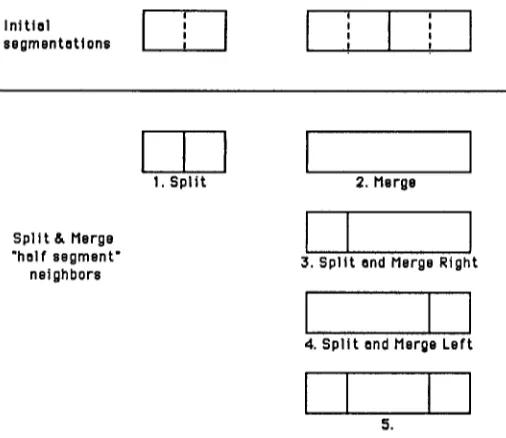
Figure 1: Split and Merge segmentation neighbors

dendrogram[11] is of the latter form. The method is a merging scheme that tries to minimize some measure of spectral dissimilarity and constrain the segmentation space for the fi- nal search. Similar search methods have also been used for image segmentation and are referred to as region growing techniques.

A Split a n d M e r g e A l g o r i t h m

In this paper we propose to use a combined split and merge strategy for the JSR problem. Such a method has originally been used for image segmentation [3]. This approach has a search neighborhood that is the union of the neighborhoods of the splitting and merging methods discussed previously. The advantages of such a method are first that it is harder to fall into local optima because of the larger neighborhood size and second that it converges faster, if we assume that we start from a point closer to the true segmentation than the top or the bottom.

To relate this algorithm to the general family of local search algorithms, consider the neighborhood that consists of segmentations with segments restricted to be not smaller than half the size of the segments in the current segmentation. In Figure 1 we show the corresponding single and two segment neighbors over one and two segments that also belong to the exact neighborhood. In the same way, we can define the "half segment" neighbors over three or more consecutive segments. As we shall see though, we found that extending the search above two-segment neighbors was un- necessary. The original split and merge neighborhood consists of neighbors 1 and 2 in Figure 1. We can either split a segment in half (at the middle frame) or merge it with the next segment. Let us denote the corresponding neighborhoods by Ns (S), Nm(S). Then the basic Split and Merge algorithm consists of a local search over all segmentations in the union of

N6(S)

and Nm(S). Furthermore, we choose

to follow a "steepest ascent" search strategy, rather than a first improvement one. Specifically, given that the segmentation at iteration k is Sk, we choose to replace it with the segmentation Sk+1

S~÷1 = arg max

I(S)

S E No (Sh)u N., (Sh)

if it improves the current score,/(Sk+l) >

l(Sk).

Convergence in a finite number of steps is guaranteed because at each step the likelihood can only increase and there are only a finite number of possible steps.

Improvements to the basic algorithm

Several other modifications to the basic algorithm were considered to help avoid local optima. We found it useful to change our splitting scheme to a two step process: first, the decision for a split at the middle point is taken, and then the boundary between the two children segments is adjusted by examining the likelihood ratio of the last and first distributions of the corresponding models. The boundary is finally adjusted to the new frame if this action increases the likelihood. This method does not actually increase the search neighborhood, because boundary adjustment will be clone only ff the decision for a split was originally taken. However, it was adopted as a good compromise between computational load and performance.

A second method that helped avoid local optima was the use of combined actions. In addition to single splits or merges, we search over segmentations produced by splitting a segment and merging the first or second half with the previous or next segment respectively. In essence, this ex- pands the search neighborhood by including the neighbors 3 and 4 in figure 1.

We also considered several other methods to escape local optima, like taking random or negative steps at the end. However, since the performance of the algorithm with the previous improvements was very close to the optimum as we shall see, the additional overload was not justified.

Constrained searches

In this section, we describe how the split and merge search can be constrained when the phones are not independent, for example when bigram probabilities are used. So far, the independence assumption allowed us to associate the most likely candidate to each segment and then perform a search over all possible segmentations. When this assumption is

t is t associated to the segment s,. no longer valid, the cost c~.

not unique for all possible segmentations that include this segment, so the search must be performed over all possible segmentations and phone sequences. For the DP search, if bigram probabilities of the form P(ak+llak) are used, the search should be done over all allowable phone durations and all phone labels at each time, which means that the search space size is multiplied by the number of phone models. A suboptimal search can be performed with the split and merge segmentation algorithm as follows:

[image:4.612.52.305.43.262.2]

(5)

and all segmentations in the search neighborhood, without using the constraint probabilities (we make the assumption that we have probabilistic constraints, in the form of a statis- tical grammar as above). Next, an action (split or merge) is taken if by changing only the phone labels of the segments the global likelihood is increased, this time including the constraint probabilities. This guarantees that the likelihood of the new segmentation is bigger than the previous one. If the decision is to take the action, we fix the segmentation and then perform a search over the phone labels only. For example, if we use bigram probabilities, this can be done with a Dynamic Programming search over the phonetic labels with the acoustic scores of the current segmentation. This last step is necessary, because once an action is taken and a local change is made, we are not guaranteed that the current scenario is globally optimum for the given segmentation because of the constraints (e.g. independent phones). As in the independent phone case, convergence of the algorithm is ensured because after each iteration of the algorithm a new configuration will be adopted only if it increases the likelihood.

In the case of non-independent phones, the exact minimal search neighborhood can be shown to be the set of all segmentations. It is therefore much easier for a local search algorithm to get trapped into local optima. For this reason, it is important that for constrained searches the above mentioned algorithm starts with a good initial segmentation. In practice we obtained a good starting segmentation by first running an unconstrained search using only unigram probabilities and incorporating the constraints as mentioned above in a second pass.

Complexity

The size of the search neighborhood at each iteration of the split and merge algorithm is

O(n),

with n the number of current segments. However, if the scores at each iteration of the algorithm are stored, then the number of segment score evaluations as defined in (3) has the order of the number of iterations with an additional initial cost. In the case of constrained searches, we can argue that there may exist pathological situations where all possible configurations are visited, and the number of iterations is exponential with N . As we shall see though, we found experimentally that the number of iterations was roughly equal to n.

R e s u l t s

The methods that we presented in this paper were evaluated on the TIMIT database [4]. The phone-classifier that we used in our experiments was identical to the baseline system described in [2]. We used Mel-warped cepstra and their derivatives together with the derivative of log power. The length of the segment model was M = 5 and had independent samples. We used 61 phonetic models, but in counting errors we folded homophones together and effectively used the reduced CMU/MIT 39 symbol set. However, we did not remove the glottal stop Q in either training or recognition, and allowed substitutions of a closure-stop pair by the

corresponding single closure or stop as acceptable errors. Those two differences from the conditions used in [5, 8] have effects on the performance estimates which offset one another.

The training and test sets that we used consist of 317 speakers (2536 sentences) and 103 speakers (824 sentences) respectively. We report our baseline results on this large test set, but our algorithm development was done on a subset of this set, with 12 speakers (96 sentences), and the comparison of the split and merge algorithm to the DP search is done on this small test set.

DP / Split and Merge comparison

The average sentence length in our small test set was 3 seconds, or 300 flames when the cepstral analysis is done every 10 msec. The number of segment score evaluations per sentence for a DP search is 15,000 when we restrict the length of the phones to be less than 50 frames, and can be reduced to approximately 4,000 if we further restrict the accuracy of the search to 2 frames. In addition, for 61 phone models and a M = 5 long segment, there are 90,000 different Gaussian score evaluations under the frame independence assumption that will eventually be computed during the DP search.

The average number of iterations for the non-constrained split and merge search over these sentences was 114, with 750 segment and 40,000 Gaussian score evaluations, when we also include the fast classification scheme. The split and merge search was on average 3 times faster than a two frame accurate DP search under these conditions, and 5 times faster than a single frame accurate DP search. Furthermore, the savings increase with the length of the model: we verified experimentally that doubling the length of the model had little effect on the split and merge search, whereas it doubled the recognition time of the DP search.

The computation savings remain the same in the case of constrained searches also. The additional segment and frame score evaluations in the second phase of the split and merge are offset by the increased search space in the DP search. Finally, we should notice that the fast classification scheme has only a small effect when a DP search is used.

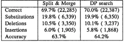
A fast suboptimal search for the JSR problem is justified if the solutions it provides are not far from the global optimum. Starting with a uniform initial segmentation near the bottom of the tree, we found that the split and merge search had almost identical performance to the DP search, without and with the bigram probabilities. The results on our small test set are summarized in Table 1, counting substitutions and deletions as errors in percent correct and with accuracy defined to be 100% minus the percentage of substitutions, deletions and insertions.

Baseline results and Discussion

(6)

Unigram

Bigram

1-Frame DP 2-Frame DP Split & merge

Segment/Frame Score Eval. 15,000/90,000

3,750180,000 750/40,000

Correct /Accuracy 70.5 / 64.8 70.6 / 64.9 69.7 / 64.6 2-Frame DP 3,750180,000 72.3 / 66.7 Split & merge 950160,000 71.9 / 66.7

Table 1: DP - Split and Merge comparison

full 61 TIMIT symbol set our recognition rate is 60% correct/54% accuracy. On the reduced symbol set, our baseline result of 70% correct/64% accuracy compares favorably with other systems using context independent models. For example, Lee and Hon [5] reported 64% correct/53% accuracy on the same database using discrete density HMMs. Their recognition rate increases to 74% correct/66% accuracy with right-context-dependent phone modelling. Lately, Robinson and Fallside [8] reported 75% correct/69% accuracy using connectionist techniques. Their system also uses context information through a state feedback mechanism (left context) and a delay in the decision (right context).

In conclusion, we achieved the main goal of this work, a significant computation reduction for connected phone recognition using the SSM with no loss in recognition performance. Our current recognition rate is close to that of systems that use context dependent modelling. However, we expect to achieve significant additional improvements when we incorporate context information and time correlation in the segment model.

A c k n o w l e d g m e n t

This work was jointly supported by NSF and DARPA under NSF grant # IRI-8902124.

References

[1] L.Bahl, P.S.Gopalakrishnan, D.Kanevsky

and D.Nahamoo, "Matrix Fast Match: A Fast Method for Identifying a Short List of Candidate Words for Decoding", in IEEE Int. Conf. Acoust., Speech, Signal Processing, Glasgow, Scotland, May 1989.

[2] V. Digalakis, M. Ostendorf and J. R. Rohlicek, "Im- provements in the Stochastic Segment Model for Phoneme Recognition," Proceedings of the Second

DARPA Workshop on Speech and Natural Language, pp. 332-338, October 1989.

[3] S. L. Horowitz and T. Pavlidis, "Picture segmentation by a tree traversal algorithm," Journal Assoc. Comput. Mach., Vol. 23, No. 2, pp. 368-388, April 1976. [4] L.F. Lamel, R. H. Kassel and S. Seneff, "Speech

Database Development: Design and Analysis of the Acoustic-Phonetic Corpus," in Proc. DARPA Speech Recognition Workshop, Report No. SAIC-86/1546, pp.

100-109, Feb. 1986.

[5] K.-F. Lee and H.-W. Hon, "Speaker-independent phone recognition using Hidden Markov Models," IEEE Trans. on Acoust., Speech and Signal Proc., Vol. ASSP- 37(11), pp. 1641-1648, November 1989.

[6] M. Ostendorf and S. Roucos, "A stochastic segment model for phoneme-based continuous speech recognition," In IEEE Trans. Acoustic Speech and Signal Pro- cessing, ASSP-37(12): 1857-1869, December 1989.

[7] C.H.Papadimitriou and K.Steiglittz, Combinatorial Op- timization, Algorithms and Complexity, Prentice-Hall, New Jersey 1982.

[8] T. Robinson and F. Fallside, "Phoneme Recognition from the TIMIT database using Recurrent Error Propa- gation Networks," Cambridge University technical report No. CUED/F-INFENG/TR.42, March 1990. [9] S. Roucos and M. Ostendorf Dunham, "A stochastic

segment model for phoneme-based continuous speech recognition," In IEEE Int. Conf. Acoust., Speech, Sig- nal Processing, pages 73-89, Dallas, TX, April 1987. Paper No. 3.3.

[10] S. Roucos, M. Ostendorf, H. Gish, and A. Derr, "Stochastic segment modeling using the estimate- maximize algorithm," In IEEE Int. Conf. Acoust., Speech, Signal Processing, pages 127-130, New York, New York, April 1988.

[11] V. Zue, J. Glass, M. Philips and S. Seneff, "Acoustic segmentation and Phonetic classification in the SUM- MIT system," in IEEE Int. Conf. Acoust., Speech, Sig- nal Processing, Glasgow, Scotland, May 1989.

Correct Substitutions Deletions Insertions Accuracy

Split & Merge DP search

69.7% (22,285) 19.8% (6,339) 10.5% (3,350) 6.0% (1,905)

63.7%

70.0% (22,387) 19.9% (6,350) 10.1% (3,237) 5.8% (1,868)

64.2%

[image:6.612.77.289.52.121.2] [image:6.612.80.282.648.717.2]