Application of Response Surface and Factorial Regression Models in Estimating Global Solar Radiation and Ultraviolet Index

ISSN 2286-4822 www.euacademic.org

Impact Factor: 3.4546 (UIF) DRJI Value: 5.9 (B+)

Application of Response Surface and Factorial

Regression

Models in Estimating Global Solar

Radiation and Ultraviolet Index

GHADA I. EL-SHANSHOURY

Radiation Safety Department Nuclear and Radiological Regulatory Authority (NRRA) Cairo, Egypt

Abstract:

This study is intended to develop predictive models for estimating monthly and daily clear sky global solar radiation on a horizontal surface (H)and maximum ultraviolet index (UVImax) for some cities in Egypt. Choosing the preferred model depends on the best and most accurate results. The applicable empirical regression models are confined in multiple linear regression model, factorial regression model and response surface regression model. The investigated models are applied for forecasting daily and monthly clear sky global solar radiation and maximum UVI for cities of Sharm El-Sheikh, Aswan, Safaga and Cairo. The new developing predictive models are calibrated. The regression models for estimating global solar radiation are based on three major predictor variables and their interactions. The predictor variables are cosine solar zenith angle at mid-time between sunrise and solar noon (cos(



_ZMT)), average air temperature (

T

) and maximum possible sunshine duration (S0). The developed

empirical models are considered as a simplified statistical approach for daily estimation of

H

because they depend on two monthly

constant parameters (S0 &

cos(



_ZMT

)

) and one daily changeable

predictive models. The results of the developed models show that the factorial regression models and the response surface regression models give more precised results than the multiple linear regression models. The predicted results of global solar radiation and maximum ultraviolet index overlap the measured data in all months of the year.

Key words: Ultraviolet index, Clear sky global solar radiation,

Cosine solar zenith angle, Air temperature and Maximum possible sunshine duration.

1. INTRODUCTION

Ultraviolet (UV) radiation is a form of electromagnetic radiation. The main source of UV radiation (rays) is the sun, although it can also come from man-made sources such as tanning beds and welding torches (American Cancer Society). Ionizing radiation is made up of energetic subatomic particles, ions or atoms moving at high speeds,

and electromagnetic waves on the high-energy end of

the electromagnetic spectrum. Gamma rays, X-rays, and the higher ultraviolet part of the electromagnetic spectrum are ionizing (Wikipedia, ionizing radiation). Higher energy UV rays often have enough energy to remove an electron from (ionize) an atom or molecule, making them a form of ionizing radiation (American Cancer Society), whereas the lower ultraviolet part of the electromagnetic spectrum and all the spectrum below UV, including

visible light (including nearly all types

of laserlight), infrared, microwaves, and radio waves are considered non-ionizing radiation (Wikipedia, ionizing radiation).

observation values are missing. The values of solar radiation in clear skies are useful for determination of the maximum performance heating and photovoltaic, moreover, for the design of air conditioning equipment in buildings or for the determination of thermal load their solar installations (El Mghouchi et al 2014).

The ultraviolet is a part of the solar spectrum (UV) that plays an important role in many processes in the biosphere. It has several beneficial influence but it may also be very harmful if UV exceeds ”safe” levels. If the amount of UV radiation is enough high the self-protection ability of some biological kinds is exhausted and the subject may be severely damaged. This is also concerned to the human organism, in specific the skin and the eyes. To avoid the harm from high UV exposures, people should limit their exposure to solar radiation by using protective procedures. The need to reach the public with simple-to-understand information about UV and its possible hazardous effects led scientists to define a parameter that can be used as an indicator of the UV exposures. This parameter is called the UV Index (UVI). It is associated to the erythemal effects of solar UV radiation on human skin (Vanicek et al 1999).

Operational UVI forecasting has already been executed in many countries. The forecast methods vary from simple statistical methods has utilized for local areas to more complicated methods with global coverage and with forecast times from a few hours to several days, either for clear sky or all sky conditions (Vanicek et al 1999).

Several researchers have developed statistical models to predict monthly global solar radiation on a horizontal surface (H) using multiple linear regression equations with different independent variables (predictor variables). Some of these predictors (weather parameters) are represented in, mean relative sunshine duration (S/S0), mean daily maximum temperature (Tmax), mean daily relative humidity (Rh), mean daily rainfall (R), mean daily temperature (

T

), ratio of maximum and minimum daily temperature and other weather parameters (Falayi et al 2008, Augustine and Nnabuchi 2009, Habbib 2011, Ituen et al 2012 , Chen and Li 2012, Adhikari et al 2013, Namrata et al 2016).

El-shanshoury et al (2017), developed the model with multiple regression equation for Sharm El-Sheikh city. This model differs from other searchers empirical models that predict the monthly clear sky monthly global solar radiation future time(H). The developed multiple linear regression model is based on three predictor parameters as independent variables. These parameters are: monthly average cosine solar zenith angle at mid-time between sunrise and solar nooncos(



_ZMT), monthly average daily mean temperature (T )

and monthly average day length (S0). Two predictors are calculated (S0 &cos(



_ZMT)) and one predictor is measured (T). This model is

considered as a simplified statistical approach for daily estimation of

H

because it depends on two monthly constant predictors (S0 &

ZMT

statistical prediction UVImax model is based on two independent variables for constructing the multiple linear regression equation. The first predictor is the monthly mean daily clear sky global solar radiation on a horizontal surface(H)and the second predictor is monthly average maximum temperature (

max

T ). After trying many

weather parameters for modeling UVImax, The model’s predictors found more parameters that are accurate for UVImax forecasting results than other parameters.

In this work new developed models are utilized with the same parameters of our previous work for estimating

H

and UVImax. The regression models are restricted in multiple linear regression model, factorial regression model and response surface regression model.

2. MATERIALS AND METHODS

The material data of monthly averaged clear sky global radiation on a horizontal surface (

H

in kWh/m2_{/day) and monthly average air mean}

and maximum temperature at 10m above the earth (

T

& Tmax in degrees celsius) is obtained from NASA meteorology (NASA). The data covered a period of 22 years (1983 – 2005) for Sharm El-Shiekh, Aswan Safaga and Cairo in Egypt. The latitude and longitude for Sharm El-Shiekh are 27.912o _{and 34.33}o_{, respectively, for Aswan are}

24.0908°and 32.8994°, for Safaga are 26.7453° and 33.95059°, and for Cairo are 30.06263° and 31.24967°. Maximum UVI data is obtained fromweather2travel-climate guides (weather2travel).

Multiple regression designs are restricted to continuous predictor (independent) variables, as main effect ANOVA designs are to categorical predictor variables. Multiple regression designs contain the separate simple regression designs for 2 or more continuous predictor variables. The regression equation for a multiple regression design for the first-order effects includes 3 continuous predictor variables C, T and S is

Y = b0 + b1C + b2T + b3S (Hill and Lewicki 2007).

Factorial regression designs are similar to factorial

ANOVA designs, in which amalgamation of the levels of the factors are represented in the design. In factorial regression designs, there may be many more such possible combinations of distinct levels for the continuous independent variables than there are cases in the data set. That is, full-factorial regression designs are defined as designs in which all possible products of the continuous predictor variables are represented in the design. For example, the full-factorial regression design for two continuous predictor variables C and T will include the main effects (i.e., the first-order effects) of C and T and their 2-way C by T interaction effect, which is represented by the product of C and T scores for each case. The regression equation is Y = b0 + b1C + b2T + b3C*T. Factorial regression designs can also be fractional, that is, higher-order effects can be omitted from the design. A fractional design for 3 continuous predictor variables C, T and S will include the main effects and all 2-way interactions between the predictor variables is

Y = b0 + b1C + b2T+ b3S+ b4C*T + b5C*S + b6T*S (Hill and Lewicki 2007).

Response surface regression Quadratic response surface

Y = b0 + b1C + b2C2 + b3T+ b4T2 + b5S+ b6S2 + b7C*T + b8C*S + b9T*S (Hill

and Lewicki 2007).

The suggested modified empirical model of clear sky global solar radiation has been estimated on the basis of measurements of monthly averaged clear sky global radiation on a horizontal surface and monthly average air mean temperature for under investigation states. Also, the empirical model is based on calculation of monthly mean daily extraterrestrial radiation and monthly average cosine solar zenith angle at mid-time between sunrise and solar noon and maximum possible sunshine duration for each state.

2.1. Empirical regression models to estimate monthly average

daily clear sky global radiation

(

H

)

The devolved regression models for estimating

H

are based on three

major predictor variables and their interactions. The major predictor parameters are

cos(



_ZMT

)

, T and S0 . The response variable is monthly averaged clear sky insolation clearness index that calculated to be predictable of

H

. Five empirical models are applied to estimate the monthly and daily average clear sky global radiation.

H

is

modeled as follow:

2.1.1. Predictive Multiple Linear Regression (MLR)model

The first-order regression model for three continuous predictor variables (C,T and S) takes the form

Model 1:

0

H

H

= b0 + b1C + b2T + b3S (1) estimated

H

= (b0 + b1C + b2T + b3S)*

H

_{0 (2)}

2.1.2. Predictive Factorial Regression (FR) model

Model 2:

0

H

H

= b0 + b1C + b2T + b3C*T (3) estimated

H

= (b0 + b1C + b2T + b3C*T)*

H

_{0 (4)}

The interaction regression model for three continuous predictor variables (C,T and S) takes the form

Model 3:

0

H

H

= b0 + b1C + b2T + b3S + b4C*T + b5C*S + b6T*S (5) estimated

H

= (b0 + b1C + b2T + b3S + b4C*T + b5C*S + b6T*S)*

H

_{0 (6)}

2.1.3. Predictive Response Surface Regression (RSR) model

The second-order polynomial regression model for two continuous predictor variables(C and T) takes the form

Model 4:

0

H

H

= b0 + b1C + b2C

2 _{+ b3T + b4T}2 _{+ b5C*T (7)}

estimated

H

= (b0 + b1C + b2C2 + b3T + b4T2 + b5C*T)*

H

₀

(8)

The second-order polynomial regression model for three continuous predictor variables (C, T and S)takes the form

Model 5:

0

H

H

= b0 + b1C + b2C

2 _{+ b3T + b4T}2 _{+ b5S+ b6S}2 _{+ b7C*T + b8C*S + b9T*S (9)}

estimated

H

= (b0 + b1C + b2C2 + b3T + b4T2 + b5S+ b6S2 + b7C*T + b8C*S + b9T*S)*

H

₀

(10)

Where, b’s are the coefficients of predictor variables, 0

H

H is monthly

average clear sky insolation clearness index,

H

is the measure of monthly mean daily clear sky global solar radiation on a horizontal surface,

H

₀ is monthly mean daily extraterrestrial radiation KW/m2_,

between sunrise and solar noon

cos(



_ZMT

)

, T represents monthly average daily mean temperature , S represents monthly average day length (S0 ) and

T

is daily mean temperature.

The values of the monthly average daily extraterrestrial radiation (

H

₀) can be calculated from the following equation (Duffie and Beckman 2013).

0 0

24

cos cos sin sin sin

180

s

SC s

w

H I E   w   



 

 _  _

  (11)

0

360

1 0.033 cos

365

n d E   _ _

 

where, ISC is the solar constant (=1.367 KWm-2_),



_{is the latitude of}

the site, δ is the solar declination, ws is the mean sunrise hour angle for the given month, and dn is the number of days of the year starting from the first of January (the Julian day number) .

The solar declination (δ) and the mean sunrise hour angle (ws) can be calculated by the following equations:

(

284)

23.45sin 360

365

n

d







_





_





,





1

cos

tan tan

s

w











The maximum possible sunshine duration (S0) (or monthly average day length) which is related to ws, can be computed by using the following equation:

0

2

15

s

S



w

(12)

Monthly average cosine solar zenith angle at mid-time between sunrise and solar noon is calculated according the following formula (NASA).

cos(θZMT) = f + g[(g - f) / 2g]½ ₍₁₃₎

where, f = sin(



)sin(δ) , g = cos(



)cos(δ)

Average daily mean temperature (

T

) is calculated as follows:

max min

( )

2

imum imum

T T

The estimated daily estimating daily clear sky global solar radiation on a horizontal surface (H) is derived from monthly

H

estimation model.

2.2. Empirical regression models to estimate the monthly

maximum ultraviolet index(UVImax)

The statistical forecasting models for estimation of monthly average maximum ultraviolet index are based on two parameters to construct the regression models. The first parameter isH_estimatedand the second

parameter isT_max. Models 6-8 present the investigated forecasting

models.

2.2.1. Predictive multiple linear regression model Model 6:

UVImax = β0+ β 1

H

+ β 2

T

_max (15)

2.2.2. Predictive factorial regression model

Model 7: UVImax = β 0+ β 1

H

+ β 2

T

_max+ β 3

H T

*

_max (16)

2.2.3. Predictive response surface regression Model 8: UVImax = β 0+ β 1

H

+ β 2

T

_max+ β 3

H

2+ β 4 2

max

T

+ β 5

H T

*

max

(17)

Where, β’s are the coefficients of predictor variables,

H

and T_maxare

considered more accurate effective for UVImax forecastingresults than other weather parameters.

2.3. Statistical evaluation

(Al-Hassany 2014, El-Mghouchi et al 2014 ). A positive MBE value means an over-estimation of the estimated values and a negative value means an under-estimation of the estimated values (Tian et al 2018).The RMSE is always positive; this test provides information on the short-term performance of the correlation by arranging a term by term comparison of the real differences between the estimated values and the measured values (Almorox 2011).RMSE is a good measure of precision. The MAPE is an overall measure of forecast accuracy (Almorox 2011), computed from the absolute mean relative difference between the global solar radiation of the measured data and those estimated by proposed model (El-Mghouchi et al 2014 ). The MABE gives the absolute value of bias error and it is a measure of the correlation goodness (Almorox 2011). It is recommended that a zero value for MBE is ideal while a low RMSE, MABE and MAPE are desirable.The correlation coefficient reflects the quality of the model; the higher CC (closed to 1), the highest model quality. The expression of each statistical indicator is given in the following forms (Almorox 2011). 1 1 , , , ,

,

,

i i

i estimated i measured N

i estimated i measured N n n H H H H

MBE

MABE

                 





1 , ,

, , 1 2 2 , , 1 1 2 ( ( )( ) ( ) ( )

i i estimated i measured

N n

i estimated estimated i measured measured i

n n

i estimated estimated i measured measured

i i

n

H H

RMSE

H H H H

CC

H H H H

                 _  _       







, , 1 ,

Where, is Number of the observations.

1

*100,

n

i measured i estimated

i i measured

N

H H

MAPE

N  H







3. RESULTS AND DISCUSSION

3.1. Empirical regression models and the prediction of

Various meteorological data are related to monthly average clear sky

clearness index

 

0

H

H . Empirical models are developed to estimate

monthly and daily global radiation.

3.1.1. Empirical development regression models for estimating monthly average clear sky clearness index

Regression analysis of five models is employed to estimate the monthlyaverage clear sky global solar radiation

(

H

)

. The empirical models are equations 1, 3, 5, 7 and 9. The following tables (1-4) show the coefficients of the empirical regression models to estimate

0 H

H for Sharm El-Sheikh, Aswan, Safaga and Cairo, respectively.

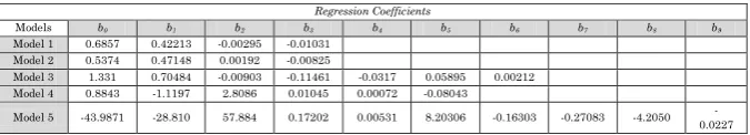
Table 1: The coefficients of the empirical regression estimation models for Sharm El-Sheikh

Regression Coefficients

Models b0 b1 b2 b3 b4 b5 b6 b7 b8 b9

Model 1 0.6857 0.42213 -0.00295 -0.01031

Model 2 0.5374 0.47148 0.00192 -0.00825

Model 3 1.331 0.70484 -0.00903 -0.11461 -0.0317 0.05895 0.00212

Model 4 0.8843 -1.1197 2.8086 0.01045 0.00072 -0.08043

Model 5 -43.9871 -28.810 57.884 0.17202 0.00531 8.20306 -0.16303 -0.27083 -4.2050 _0.0227

-Table 2: The coefficients of the empirical regression estimation models for Aswan

Regression Coefficients

Models b0 b1 b2 b3 b4 b5 b6 b7 b8 b9

Model 1 0.5203 -0.01807 0.79727 -0.00353

Model 2 0.0960 1.1528 0.01204 -0.02533

Model 3 -1.8382 4.9737 -0.01216 0.17303 -0.04217 -0.3379 0.00294

Model 4 0.2255 0.4241 1.8283 0.01918 0.00065 -0.0882

Model 5 -35.6882 7.4866 39.6735 -0.05842 -0.0007 5.63753 -0.07642 -0.00571 -5.4167 0.0079

Table 3: The coefficients of the empirical regression estimation models for Safage

Regression Coefficients

Models b0 b1 b2 b3 b4 b5 b6 b7 b8 b9

Model 1 0.45123 0.14168 -0.00578 0.02337

Model 2 0.77901 0.04318 -0.01659 0.01821

Model 3 1.72539 2.60898 -0.05447 -0.19866 -0.06797 -0.02137 0.007618

Model 4 1.210684 -2.12527 3.761624

3.06E-05 0.000929 -0.08158

Table 4: The coefficients of the empirical regression estimation models for Cairo

Regression Coefficients

Models b0 b1 b2 b3 b4 b5 b6 b7 b8 b9

Model 1 0.51251 0.25875 -0.00499 0.008132

Model 2 0.62571 0.22771 -0.00937 0.007464

Model 3 1.23308 -0.1230 -0.00957 -0.0800 -0.00707 0.07803 0.000735

Model 4 0.73562 -0.3226 0.73023 -0.00517 9.6E-05 -0.00653

Model 5 -44.0632 -10.8823 73.8287 -0.03741 -0.00086 7.73516 -0.08363 0.01431 -7.8058 0.00502

3.1.2. Statistical evaluation of the regression models

The results of the validation of the five models that estimate

H

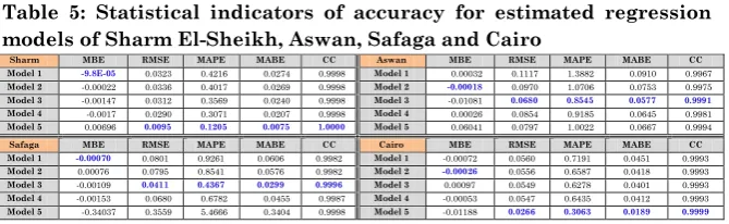
for Sharm El-Sheikh, Aswan, Safaga and Cairo cities are shown in Table 5.

Table 5: Statistical indicators of accuracy for estimated regression models of Sharm El-Sheikh, Aswan, Safaga and Cairo

Sharm MBE RMSE MAPE MABE CC Aswan MBE RMSE MAPE MABE CC Model 1 -9.8E-05 0.0323 0.4216 0.0274 0.9998 Model 1 0.00032 0.1117 1.3882 0.0910 0.9967

Model 2 -0.00022 0.0336 0.4017 0.0269 0.9998 Model 2 -0.00018 0.0970 1.0706 0.0753 0.9975

Model 3 -0.00147 0.0312 0.3569 0.0240 0.9998 Model 3 -0.01081 0.0680 0.8545 0.0577 0.9991 Model 4 -0.0017 0.0290 0.3071 0.0207 0.9998 Model 4 0.00026 0.0854 0.9185 0.0645 0.9981

Model 5 0.00696 0.0095 0.1205 0.0075 1.0000 Model 5 0.06041 0.0797 1.0022 0.0667 0.9994

Safaga MBE RMSE MAPE MABE CC Cairo MBE RMSE MAPE MABE CC Model 1 -0.00070 0.0801 0.9261 0.0606 0.9982 Model 1 -0.00072 0.0560 0.7191 0.0451 0.9993

Model 2 0.00076 0.0795 0.8541 0.0576 0.9982 Model 2 -0.00026 0.0556 0.6587 0.0418 0.9993

Model 3 -0.00109 0.0411 0.4367 0.0299 0.9996 Model 3 0.00097 0.0549 0.6278 0.0401 0.9993

Model 4 -0.00153 0.0680 0.6782 0.0455 0.9987 Model 4 -0.00053 0.0547 0.6435 0.0412 0.9993

Model 5 -0.34037 0.3559 5.4666 0.3404 0.9998 Model 5 -0.01188 0.0266 0.3063 0.0189 0.9999

The obtained results of Sharm El-Sheikh and Cairo show that there are a remarkable agreement between the measured and predicted values using different regression models except Model 5 (the second-order polynomial regression model for three continuous predictor variable). This model gives high accurate results than other models according to the values of RMSE, MAPE, MABE and CC.

The suitable model for Aswan and Safaga cities is different than the suitatble one for Sharm El-Sheikh and Cairo. The interaction regression model for three continuous predictor variables (Model 3) fits Aswan and Safaga more than other regression models.

low values of these mean errors are desirable, though it should be noted that over-estimation of an individual data element will cancel under-estimation in a separate observation (Almorox 2011).

3.1.3. The predictive model to estimate monthly average clear sky global solar radiation

(

H

)

From the previous analysis of models validation, the best model for estimating the

H

is the model that has three continuous predictor

variables. The monthly average clear sky global solar radiation on a horizontal surface for each investigated cityis:

For Sharm El-Sheikh, the response surface regression model (model 5, Table 1).

estimated

H

= (-43.9871 - 28.810C + 57.884C2 _{+ 0.17202T + 0.00531T}2 _{+ 8.20306S -}

0.16303S2 _{- 0.27083C*T – 4.2050C*S - 0.0227T*S)*}

0

H

For Aswan, the factorial regression model (model 3, Table 2).

estimated

H

= (-1.8382+ 4.9737C - 0.01216T + 0.17303S - 0.04217C*T - 0.3379C*S +

0.00294T*S)*

H

₀

For Safaga, the factorial regression model (model 3, Table 3).

estimated

H

= (1.72539+ 2.60898C - 0.05447T - 0.19866S - 0.06797C*T - 0.02137C*S +

0.007618*S)*

H

₀

For Cairo, the response surface regression model (model 5, Table 4).

estimated

H

= (-44.0632-10.8823C + 73.8287C2 _{-0.03741T - 0.000861T}2 _{+7.73516S -}

0.08363S2_{+ 0.01431C*T – 7.8058C*S + 0.00502T*S)*}

0

H

3.1.4. The results of

H

_estimated of the best selected model in each

The values of H₀,

0

H

H , cos(



ZMT),

T

, S0, and

H

estimated are

presented in Table 6-10.

H

_estimatedis calculated form the best selected models (Model 5 for Sharm El-Sheikh & Cairo, and Model 3 for Aswan & Safaga (the equations given in the previous section).

Table 6: Monthly average meteorological data and clear sky global solar radiation for Sharm El-Sheikh using Model 5

MONTH Hmeasured

(KW/m2/day)

0

H

(KW/m2/day) 0

measured

H

H cos(ZMT) T S0

0

estimated H

H H(KW/mestimated2/day)

JAN 4.55 6.2563 0.72727 0.47335 15.8 10.4467 0.7295 4.564

FEB 5.58 7.4431 0.74969 0.53653 16.5 11.0364 0.7507 5.587

MAR 6.88 8.9678 0.76719 0.61038 19.6 11.8304 0.7695 6.901

APR 7.88 10.308 0.76443 0.66447 24.0 12.6801 0.7652 7.888

MAY 8.34 11.089 0.75206 0.68588 27.7 13.3882 0.7534 8.355

JUN 8.53 11.349 0.75163 0.68930 30.0 13.7394 0.7518 8.532

JUL 8.30 11.187 0.74197 0.68823 31.3 13.5742 0.7426 8.307

AUG 7.84 10.556 0.74270 0.67545 31.4 12.9619 0.7424 7.837

SEPT 6.98 9.3964 0.74284 0.63373 30.1 12.1415 0.7429 6.980

OCT 5.69 7.8727 0.72275 0.56229 26.5 11.2938 0.7229 5.692

NOV 4.72 6.5046 0.72564 0.48926 21.8 10.5924 0.7265 4.725

DEC 4.22 5.8725 0.71861 0.45275 17.6 10.2591 0.7194 4.225 Table 7: Monthly average meteorological data and clear sky global solar radiation for Aswan using Model 3

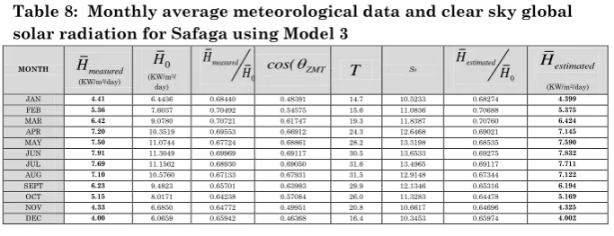
Table 8: Monthly average meteorological data and clear sky global solar radiation for Safaga using Model 3

MONTH Hmeasured

(KW/m2/day)

0

H

(KW/m2/

day) 0

measured H

H cos(ZMT) _T S0

0

estimated H

H Hestimated

(KW/m2/day)

JAN 4.41 6.4436 0.68440 0.48391 14.7 10.5233 0.68274 4.399

FEB 5.36 7.6037 0.70492 0.54575 15.6 11.0836 0.70688 5.375

MAR 6.42 9.0780 0.70721 0.61747 19.3 11.8387 0.70760 6.424

APR 7.20 10.3519 0.69553 0.66912 24.3 12.6468 0.69021 7.145

MAY 7.50 11.0744 0.67724 0.68861 28.2 13.3198 0.68535 7.590

JUN 7.91 11.3049 0.69969 0.69117 30.5 13.6533 0.69275 7.832

JUL 7.69 11.1562 0.68930 0.69050 31.6 13.4965 0.69117 7.711

AUG 7.10 10.5760 0.67133 0.67931 31.5 12.9148 0.67344 7.122

SEPT 6.23 9.4823 0.65701 0.63993 29.9 12.1346 0.65316 6.194

OCT 5.15 8.0171 0.64238 0.57084 26.0 11.3283 0.64478 5.169

NOV 4.33 6.6850 0.64772 0.49951 20.8 10.6617 0.64696 4.325

DEC 4.00 6.0659 0.65942 0.46368 16.4 10.3453 0.65974 4.002 MONTH Hmeasured

(KW/m2/day)

0 H

(KW/m2/

day) 0

measured

H

H ZMT

cos( ) _T S0

0

estimated H

H H_(KW/mestimated2/day)

JAN 4.55 6.8628 0.6630 0.50713 15.8 10.6916 0.66835 4.587

FEB 5.77 7.9584 0.7250 0.56584 16.8 11.1874 0.71999 5.730

MAR 6.89 9.3146 0.7397 0.63264 20.7 11.8569 0.74274 6.918

APR 7.72 10.4358 0.7398 0.67864 26.0 12.5737 0.73035 7.622

MAY 7.86 11.0251 0.7129 0.69370 29.9 13.1697 0.72340 7.976

JUN 8.25 11.1917 0.7372 0.69429 31.7 13.4644 0.72749 8.142

JUL 8.00 11.0731 0.7225 0.69452 32.5 13.3259 0.72113 7.985

AUG 7.47 10.6064 0.7043 0.68701 32.4 12.8112 0.70946 7.525

SEPT 6.93 9.6632 0.7172 0.65304 31.0 12.1194 0.70668 6.829

OCT 5.79 8.3337 0.6948 0.58941 27.3 11.4043 0.70027 5.836

NOV 4.76 7.0876 0.6716 0.52201 21.8 10.8139 0.66989 4.748

DEC 4.22 6.5004 0.6492 0.48779 17.4 10.5343

Table 9: Monthly average meteorological data and clear sky global solar radiation for Cairo using Model 5

MONTH Hmeasured

(KW/m2_/ day)

0

H

(KW/m2_/

day) 0

measured

H

H cos(ZMT) T S0

0

estimated H

H estimated

H

(KW/m2_/day)

JAN 3.86 5.9068 0.65349 0.45335 13.3 10.3004 0.65247 3.854

FEB 4.72 7.1401 0.66106 0.51895 13.6 10.9466 0.66164 4.724

MAR 5.99 8.7551 0.68417 0.59666 16.0 11.8147 0.68207 5.972

APR 7.07 10.2172 0.69197 0.65517 20.1 12.7433 0.69132 7.063

MAY 7.46 11.1074 0.67162 0.68006 23.4 13.5185 0.67114 7.455

JUN 7.76 11.4197 0.67953 0.68502 26.3 13.9037 0.67525 7.711

JUL 7.35 11.2325 0.65435 0.68325 28.2 13.7225 0.65592 7.368

AUG 6.89 10.5087 0.65565 0.66759 28.2 13.0517 0.64956 6.826

SEPT 5.93 9.22796 0.64261 0.62162 26.3 12.1546 0.64455 5.948

OCT 4.76 7.59878 0.62642 0.54590 22.8 11.2281 0.62252 4.730

NOV 3.85 6.16713 0.62428 0.46982 18.9 10.4603 0.62470 3.853

DEC 3.49 5.51261 0.63309 0.43207 14.8 10.0945 0.63201 3.484

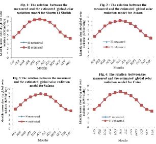
Figures 1-4 show the relation between the measured and predicted values of

H

using the suitable empirical development model for each

values of monthly average of clear sky global solar radiation. However, the estimated

H

overlaps the measured

H

in all months of

the year. Figures 1-4 illustrate also that the values in the month range May-July belong to the maximum value for the global solar radiation. Moreover, the estimated high global solar radiation of the summer months is required for detailed study to get the maximum benefits of solar energy for the production of electric power.

3.1.5. Application of the predictive regression model for estimating daily clear sky global solar radiation on a horizontal surface (H) for Cairo city

To predict the daily clear sky global solar radiation (H) in Cairo, substitute the values of

cos(



_ZMT

)

and S0, according to the

corresponding month for the day that to be predicted, in the predictive response surface regression model (Model 5, Table 4).

T

is calculated from daily changing maximum and minimum temperature (eqn. 14). For example, to predict H of few days for some months, substitute the monthly values of S0, cos(



_ZMT) and H₀ (from Table 9, for each

month which corresponding that day to be predicted) in the following equation,

estimated

H

= (-44.0632-10.8823C + 73.8287C2 _{-0.03741T - 0.000861T}2 _{+7.73516S -}

0.08363S2_{+ 0.01431C*T– 7.8058C*S + 0.00502T*S)*}

0

H

The results are presented in Table 10.

Table 10: Some estimated values of daily clear sky global solar radiation in Cairo

Date H0 cos(ZMT) T S0

0

estimated

H

H estimated

H

KW/m2_{/ day}

26-4-2018 10.2172 0.65517 (29+18)/2 = 23.50 12.743 0.68581 7.007

29-4-2018 10.2172 0.65517 (35+21.5)/2=28.25 12.743 0.64481 6.588

11-5-2018 11.1074 0.68006 (32+20)/2 = 26.00 13.519 0.66499 7.386

23-5-2018 11.1074 0.68006 (38.5+26.5)/2=32.5 13.519 0.59873 6.650

31-5-2018 11.1074 0.68006 (33+23)/2 = 28.00 13.519 0.65234 7.246

10-6-2018 11.4197 0.68502 (38.5+26)/2=32.25 13.904 0.62627 7.152

27-6-2018 11.4197 0.68502 (42.5+25)/2=33.75 13.904 0.60430 6.901

04-7-2018 11.2325 0.68325 (42+24)/2 = 33.00 13.723 0.60098 6.751

From Table 10, it should be noted that whenever the value of average day temperature increases, the value of global solar radiation decreases according to the corresponding days in the same month. That means, there is inversely relationship between the value of average temperature and the value of global solar radiation. The choice of the month range May-July is considered in this work because the effect of UVI is maximum. The prediction value of H is used for forecasting dailyvalue of UVI.

3.2. Empirical regression models and the prediction of monthly and daily maximum ultraviolet index

In this section, three models are applied to estimate the monthly average UVImax (eqns. 15-17) and are compared as attempt to deduce the best of one for each city. There is strong relationship between

H

,

max

T , as independent variable, and UVI , as dependant variable.

That refers to try substituting many weather parameters for modeling UVImax. Those model’s predictors are found to give more accurate parameters for UVImax forecasting results than other weather parameters.

3.2.1. The predictive model to estimate monthly average UVImax

From the regression analysis and according to accuracy indicators, it has been found that the factorial regression model gives the best results in estimating monthly average UVImax for Sharm El-Sheikh and Cairo. As well as, the response surface regression model gives the best results for Aswan and Safaga. The interaction and second-order polynomial regression models for two continuous predictor variables (

H

& T_max) are considered the suitable models for applications (Models

7 & 8). The best predictive model for estimation of monthly average UVImax for each investigated cityis :

For Sharm El-Sheikh,

For Aswan,

UVImax = -11.7285 + 5.5139

H

- 0.07192

T

_max- 0.22392

H

2+ 0.00879

T

_max2 _-

0.05541

H T

*

max

For Safaga,

UVImax = -27.0589 + 5.7864

H

+ 0.9889

T

_max - 1.2353

H

2 - 0.04814

T

_max2 +

0.33922

H T

*

max

For Cairo,

UVImax = -5.2032+ 1.07451

H

+ 0.24131

T

_max+ 0.0011

H T

*

_max

The results of the performance indicators show that the error rate for each predictive model is being reduced in varying proportions when compared with each other (Multiple Linear Regression (MLR) model, Factorial Regression (FR) model and response surface regression (RSR) model). The error rate of Sharm El-Sheikh predictive model is reduced by about 10% from MLR model and it has almost the same values of as those of RSR model. The error rate of Aswan predictive model is reduced by about 65% from MLR and 45% from FR models. The error rate of Safaga predictive model is reduced by about 65% from MLR and 50% from FR models. The error rate of Cairo predictive model is reduced by about 65% from MLR and 55% from RSR models. Figures 5-8 show the relationship between the measured and estimated values of monthly average UVImax using the suitable empirical developed model for each city. It is clear from the figures that there is an excellent correlation and a perfect relationship exists between the measured and estimated monthly average UVImax.

The estimated value of daily UVImax is calculated from monthly UVImax estimation models, by substituting with the value of daily

clear sky global solar radiation on a horizontal surface (

H

_estimated) and daily maximum temperature (

T

_max).

3.2.2. Application of the predictive regression model for estimating daily UVImax for Cairo city

For example, to estimate the daily value of UVImax of the same days in Table10, are has to substitute the values of

H

_estimatedand daily Tmax

(from Table 10) in the following interaction regression model (FR model):

UVImax = -5.2032+ 1.07451

H

+ 0.24131

T

_max + 0.0011

H T

*

_max

The results of daily UVImax values are presented in Table 11:

Table 11: Some estimated values of daily UVImax in Cairo

Date

H

_estimated Tmax Estimated UVImax

26-4-2018 7.007 29.0 9.547

29-4-2018 6.588 35.0 10.575

11-5-2018 7.386 32.0 10.715

23-5-2018 6.650 38.5 11.514

31-5-2018 7.246 33.0 10.809

10-6-2018 7.152 38.5 12.075

27-6-2018 6.901 42.5 12.790

04-7-2018 6.751 42.0 12.498

10-7-2018 6.991 38.0 11.771

value of UVImax increases according to each day in the same month.

That means, there is inversely relationship between UVImax and global solar radiation. In addition, there is a direct relationship between UVImax and Tmax..

3.2.3. The daily UV dose (DUVD)

It can be calculate as an integral of UV index over the daylight time

as follows:

! 0

( )

N

T

T

DUVD

UVI t dt





_

Where, To is thesunrise timeand TN+1 is the sunset time.

The calculations are performed again using the trapezoid rule that results in the following formula:

1 1

0 1

( ) ( )

2 N

j j j j

j

DUVD UVI UVI _ T_ T 





  

The daily UV dose is in UV Index hours (UVI h) if the units of Tj are in hours. To convert UVI h units to kJ/m2_{, units that are commonly} used to express DUVD, are has to multiply the result from the last equation by the factor: 0.09=25*3.6/1000 (Kiedron et al, 2007).

4. CONCLUSION

The statistical empirical estimation models of monthly and daily clear sky global radiation

(

H

(for monthly) and (for daily))

H

and maximum ultraviolet index (UVImax) is constructed for states of Sharm El-Sheikh, Aswan, Safaga and Cairo. The empirical regression models are applied and compared. The applicable predictive regression models include multiple linear regression model, factorial regression model and response surface regression model. Three major predictor parameters are employed to estimate

H

. The predictor variables are T,cos(_ZMT), S0. The response variable is the variable to

El-regression model) fits Aswan and Safaga more than other El-regression models.

The empirical H developed model is considered as a simplified statistical approach because it depends on two monthly constant parameters (S0 & cos(_ZMT)), and one daily changeable parameter ( )T

.The estimated high global solar radiation of the summer months is required for detailed study to get the maximum benefits of solar energy that to forecast UVImax and for the production of electric power. The regression estimation models of UVImax are based on two parameters. Precision of the developed forecasting model of monthly and daily UVImax is based on maximum temperature (

T

_maxfor monthly or Tmax for daily) and accurate prediction of

H

or H. The global solar radiation and maximum temperature are considered more accurate and effective for UVImax forecastingresults than other meteorological parameters. The UVImax results show that, the factorial regression model is the best for Sharm El-Sheikh and Cairo. Furthermore, the response surface regression model is more adequate for Aswan and Safaga than other models. The value of UVImax increases with the increase in the value of maximum temperature, so that the increase in the UVImax be linked to the low values of H foreach day in the same month. The month range May-July (summer) was chosen in this work because the effect of UVI is maximum. There is an excellent correlation exists between the measured and predicted values for each

of HH₀ and UVImax. Moreover, the predicted values of ₀

H

H and

UVImax match the measured data in all months of the year.

REFERENCES

1. Adhikari K. R., Bhattarai B. K. and Gurung S., (2013); Estimation of Global Solar Radiation for Four Selected Sites in Nepal Using Sunshine Hours, Temperature and Relative Humidity Journal of Power and Energy Engineering, 1, pp. 1-9. 2. Al-Hassany Gh. S., (2014); Calculated the diffuse and direct

World Models of Liu–Jordan, Iraqi Journal of Physics, Vol. 12, No. 25, PP. 94-104.

3. Almorox J., (2011); Estimating global solar radiation from common meteorological data in Aranjuez, Spain, Turk J Phys, Vol. 35, pp. 53 – 64.

4. AmbientWeather.com - Smart Weather Stations;

https://www.ambientweather.com/solarradiation.html.

5. American Cancer Society;

https://www.cancer.org/cancer/cancer-causes/radiation-exposure/uv-radiation/uv-radiation-what-is-uv.html.

6. Augustine C. and Nnabuchi M. N., (2009); Empirical Models for the Correlation of Global Solar Radiation with Meteorological Data for Enugu, Nigeria, the Pacific Journal of Science and Technology Vol. 10, No. 1, pp. 693-700.

7. Chen J. L and Li G. Sh.,(2012); Estimation of Monthly Mean Solar Radiation from Air Temperature in Combination with Other Routinely Observed Meteorological Data in Yangtze River Basin in China, Journal of Meteorological Applications, Vol. 21, Issue 2, pp. 459-468.

8. Duffie J. A. and Beckman W. A. (2013); Solar Engineering of Thermal Processing, Fourth Edition, John Wiley & Sons, Inc. 9. El-Mghouchi Y., El Bouardi A. Choulli Z. and Ajzoul T., (2014);

New Model to Estimate and Evaluate

the Solar Radiation, International Journal of Sustainable Built Environment, Vol. 3, Issue 2, pp. 225-234.

10. El-Shanshoury G., El- Shanshoury H. and Abaza A., (2017); Health Effects of Low Level Ionizing

Radiation Compared to Estimated UV index in Sharm El-Sheikh, Egypt, International Journal of Advanced Research (IJAR), Vol. 5, Issue 1, pp. 610-624.

11. Falayi E. O., Adepitan J. O. and Rabiu A. B.,(2008); Empirical Models for the Correlation of Global Solar Radiation with Meteorological Data for Iseyin, Nigeria International Journal of Physical Sciences Vol. 3. No. 9, pp. 210-216.

13. Hatfield L. A., Hoffbeck R. W., Alexander B. H. and Carlin B. P., (2009); Spatiotemporal and Spatial Threshold Models for Relating UV Exposures and Skin Cancer in the Central United States. Comput. Stat. Data Anal., Vol. 53, No. 8, pp. 3001-3015. doi: 10.1016/j.csda.2008.10.013.

14. Hill T. and Lewicki P., (2007); STATISTICS: Methods and Applications. StatSoft, Tulsa, OK. StatSoft, Inc. (Electronic

Statistics Textbook. Tulsa, OK: StatSoft.,

http://www.statsoft.com/textbook/.

15. Ituen E. E., Esen N. U., Nwokolo S. C. and Udo E. G., (2012); Prediction of Global Solar Radiation Using Relative Humidity, Maximum Temperature and Sunshine Hours in Uyo, in the Niger Delta Region, Nigeria Advances in Applied Science Research, 2012, Vol. 3, No. 4, pp.1923-1937.

16. Kiedron P., Stierle S. and Lantz K., (2007); Instantaneous UV Index and Daily UV Dose Calculations, NOAA-EPA Brewer Network.1www.esrl.noaa.gov/gmd/grad/neubrew/docs/UVin

dex.pdf.

17. Miller A. C., Satyamitra M. and Kulkarni, S. (in press), "Late and Low Level Effects of Ionizing Radiation”, Textbook of Military Medicine, Bender Press, Washington, DC [in press]. 18. Namrataa K., Sharmab S. P. and Seksenaa S. B. L., (2016);

Empirical Models for the Estimation of Global Solar Radiation with Sunshine Hours on Horizontal Surface for Jharkhand (India), Applied Solar Energy, Vol. 52, No. 3, pp. 164–172, Allerton Press, Inc.

19. NASA Surface Meteorology and Solar Energy–Choices, (2016); Atmospheric Science Data Center, Parameter Definition.

https://eosweb.larc.nasa.gov/cgi-bin/sse/grid.cgi.

20. Tian Z. , Perers B., Furbo S., Fan J., Deng J. and Dragsted J., (2018); A Comprehensive Approach for Modelling Horizontal Diffuse Radiation, Direct Normal Irradiance and Total Tilted Solar Radiation Based on Global Radiation under Danish Climate Conditions, Energies Journal, Vol. 11, 1315

Prepared by the Working Group 4 of the COST-713 Action “UVB Forecasting”.

22. Weather2travel–climate guides, Egypt Climate and Weather,

www.weather2travel.com/climate-guides/.

23. Wiegant E., Van Geffen J., van Weele M., Van Der A. R. and Houweling S., (2016); Improving Satellite Based Estimations of UV Index and Dose and First Assessment of UV in A World-Avoided. Utrecht University, Master Thesis, KNMI Scientific Report WR-2016-01. 1-65.

24. Wikipedia, Ionizing Radiation;