Pharmaceutical Process Modeling, Optimization, and Control

(1)

Western University Western University

Scholarship@Western

Electronic Thesis and Dissertation Repository

9-4-2013 12:00 AM

Pharmaceutical Process Modeling, Optimization, and Control

Ehsan Sheikholeslamzadeh The University of Western Ontario Supervisor

Sohrab Rohani

The University of Western Ontario

Graduate Program in Chemical and Biochemical Engineering

A thesis submitted in partial fulfillment of the requirements for the degree in Doctor of Philosophy

Follow this and additional works at: https://ir.lib.uwo.ca/etd

Part of the Process Control and Systems Commons, Thermodynamics Commons, and the Transport Phenomena Commons

Recommended Citation Recommended Citation

Sheikholeslamzadeh, Ehsan, "Pharmaceutical Process Modeling, Optimization, and Control" (2013). Electronic Thesis and Dissertation Repository. 1622.

https://ir.lib.uwo.ca/etd/1622

This Dissertation/Thesis is brought to you for free and open access by Scholarship@Western. It has been accepted for inclusion in Electronic Thesis and Dissertation Repository by an authorized administrator of

(2)

Pharmaceutical Process Modeling, Optimization, and

Control

(Thesis format: Integrated-Article)

By

Ehsan Sheikholeslamzadeh

Graduate Program in Engineering Science Department of Chemical and Biochemical Engineering

A thesis submitted in partial fulfillment of the requirements for the degree of

Doctor of Philosophy

The School of Graduate and Postdoctoral Studies The University of Western Ontario

(3)

ii

Abstract

(4)

iii Keywords:

(5)

iv

Co-Authorship Statement

Chapter 02: Writing the manuscript, experimental work, data gathering, and parameter estimation were performed by the author. This work was supervised by Dr. Sohrab Rohani, whose input was very important for the improvement of its content. His recommendations were incorporated in this chapter. A version of this chapter has been published in the Industrial & Engineering Chemistry Research Journal:

E. Sheikholeslamzadeh, S. Rohani. Solubility Prediction of Pharmaceutical and Chemical Compounds in Pure and Mixed Solvents Using Predictive Models, Ind. Eng. Chem. Res.

2012, 51, 464-473.

Chapter 03: The original draft of this chapter was prepared by the author. All the required data was gathered and analysed by the written codes in Matlab environment. The implementation of the models were done by the author. The valuable recommendations by Dr. Sohrab Rohani strengthened the content of the paper. A version of this chapter has been published in Fluid Phase Equilibria Journal:

E. Sheikholeslamzadeh, S. Rohani. Vapour-liquid and vapour-liquid-liquid equilibrium modeling for binary, ternary, and quaternary systems of solvents, Fluid Phase Equilib.

2012, 333, 97-105.

Chapter 04: The original draft of this chapter was prepared by the author. Further review was performed by Dr. Sohrab Rohani, whose recommendations were very helpful in improving the contents of the manuscript. Dr. Chau-Chyun Chen from Aspen Technology gave some valuable helps in performing a few revisions on the manuscript. A version of this chapter has been published in Industrial & Engineering Chemistry Research Journal:

(6)

v

Chapter 05: The original draft of this chapter was prepared by the author. Further review was performed by Dr. Sohrab Rohani, whose recommendations were very helpful in improving the contents of the manuscript. A version of this chapter has been published in Industrial & Engineering Chemistry Research Journal:

E. Sheikholeslamzadeh, S. Rohani. Modeling and Optimal Control of Solution Mediated Polymorphic Transformation of L-Glutamic Acid, Ind. Eng. Chem. Res. 2013, 52, 2633-2641.

(7)

vi

Acknowledgments

I would like to take this opportunity to acknowledge and thank those who made this work possible. First, I would like to express my appreciation to my supervisor, Dr. Sohrab Rohani, for his warm support and invaluable feedback throughout the progress of this project. He was always open to novel ideas and also provided a good atmosphere that helped me to reach my full potential. I am always grateful for that.

I deeply appreciate the recommendations and invaluable feedback from Dr. Chau-Chyun Chen from Aspen Technology regarding the solvent screening project. His advice was beneficial in revising the manuscript related to the solvent screening work.

My several thanks to all of the people in our research group whom they cooperation in doing my project lead to successful outcomes in this project.

I would like to give special thanks to my mother, father, brother, and my sisters, who never gave up to support and always, motivated me to pursue my research during my PhD at Western University. My brother helped me a lot in all aspects of my life during his stay here at Western while doing his masters in electrical engineering. I hope I have made them proud. They deserve it.

(8)

vii

List of Tables

Chapter 02

Table 2-1. NRTL binary interaction constants for conceptual segments ... 25

Table 2-2. Physical properties of the model compounds used for thermodynamic modeling and prediction ... 29

Table 2-3. Functional groups that are defined in UNIFAC and their replication in two different structures of 3-pentadecylphenol ... 31

Table 2-4. Optimized segment numbers for the model compounds using the NRTL-SAC method

... 32

Table 2-5. Experimental solubility of 3-pentadecylphenol in pure IPA and its mixtures with water ... 33

Table 2-6. Functional groups that have been used in modeling with the UNIFAC model ... 36

Table 2-7. Average relative deviation for the UNIFAC and NRTL-SAC in three methods ... 40

Table 2-8. Optimized segment numbers for each method used for NRTL-SAC model ... 40

Chapter 03

Table 3-1. Deviation of predictive model results from corresponding experimental values of Chen et al. [17] ... 55

(14)

xiii

Table 3-3. Binary solution deviation of model vs. experimental data for three pairs of Diethyl ether-Methanol-Butanol (%ARD) ... 61

Table 3-4. Average absolute deviation (%AAD) for predictive models and two correlative models for a ternary system of Diethyl Ether-Methanol-Butanol ... 62

Table 3-5. %ARD for the two quaternary systems of VLLE ... 64

Chapter 04

Table 4-1. Segment numbers, Antoine coefficients of vapour pressure, and normal boiling points of solvents studied in the current work [19] with the class number assigned to each solvent by Food and Drug Administration (FDA) [18] ... 75

Table 4-1. Continued ... 76

Table 4-2. Segment numbers and physical properties of selected components from the literature ... 83

Table 4-3. The optimal single solvent for each of model components with their starting and ending operating temperature at 40oC and 20oC, respectively ... 85

Table 4-4. Optimal conditions of operation for cooling and antisolvent crystallization for the first objective function (J) ... 91

Table 4-5. Optimum yield of first objective function (J1) for model components with its

corresponding yield based on second objective and the CPU time allocated for calculation for binary solvent optimization ... 92

Table 4-6. Optimal solvent mole ratios, volume ratios, and temperature for the start and final part of crystallization ... 95

(15)

xiv

Table 4-8. Optimal yield values for single, binary, and ternary solvent combinations ... 97

Chapter 05

Table 5-1. Kinetic parameters with their values and units ... 112

Table 5-2. Seed size distribution parameters for stable (α) and metastable (β) forms used in

equation (5-7) ... 113

Table 5-3. Optimal values of mass of stable, metastable, and the size of stable form with their values of conventional cooling policies ... 125

Table 5-4. Important results of the crystallization process using the two methods of MOC and MOMC ... 127

Chapter 06

(16)

xv

List of Figures

Chapter 01

Figure 1-1. Schematic diagram of typical processes that involved in the pharmaceutical manufacturing ... 3

Figure 1-2. Project summary with the brief title of each section ... 10

Chapter 02

Figure 2-1. The algorithm of converging to the solubility of a ternary system using UNIFAC model ... 17

Figure 2-2. Algorithm flowchart for parameter estimation using NRTL-SAC model ... 22

Figure 2-3. The chemical structure of 3-pentadecylphenol in compact form (right) and the length of bonds in Angstrom () (left) ... 24

Figure 2-4. Chemical structure of lovastatin ... 26

Figure 2-5. Chemical structure of valsartan ... 27

Figure 2-6. Characterization of re-crystallized 3-pentadecylphenol with DSC (left) and XRPD (right) ... ... 28

Figure 2-7. Experimental points of the solubility of 3-pentadecylphenol in two solvents and their curve of estimation using NRTL-SAC model. The curves of UNFAC are also shown here for comparison ... 32

(17)

xvi

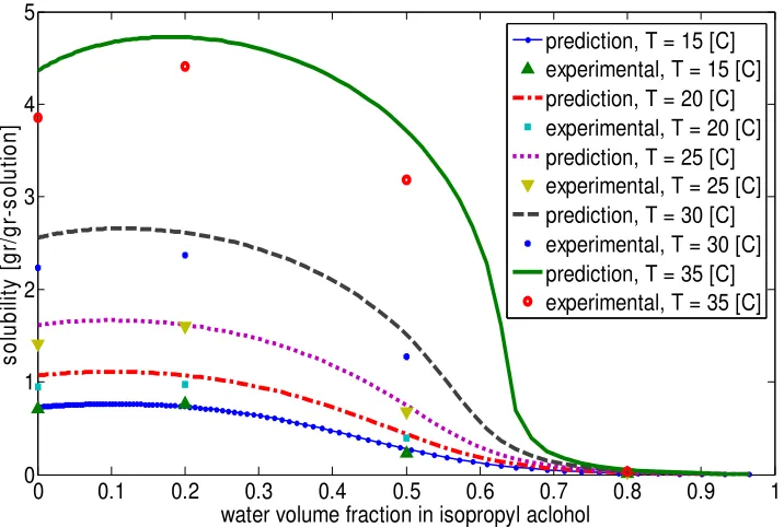
Figure 2-9. Experimental and predicted values of the solubility data of 3-pentadecylphenol in IPA-water mixture at different temperatures ... 35

Figure 2-10. Schematic view of functional groups presented in lovastatin ... 36

Figure 2-11. Experimental data with the predictions of solubility in four selected solvents using three methods of the NRTL-SAC and the UNIFAC method ... 37

Figure 2-12. Predicted and experimental values of valsartan in two solvents: left: acetonitrile, right: butyl acetate ... 39

Figure 2-13. Solubility prediction of valsartan in three ethyl acetate + hexane mixtures for different mole percent of ethyl acetate as a solvent ... 42

Figure 2-14. Schematic diagram for finding the fugacity change from solid to liquid state of a pure substance ... 43

Chapter 03

Figure 3-1. Predicted and experimental results for systems (A) ethanol-toluene at 101.3kPa, (B) ethanol-toluene at 201.3kPa, (c) isopropanol-toluene at 101.3kPa, and (D) isopropanol-toluene at 201.3kPa ... 56

Figure 3-2. Txy diagram of VLE systems; (A) ethanol-water, (B) ethanol-ethylene glycol, and (C) water-ethylene glycol all at 101.3kPa ... 57

Figure 3-3. Vapour phase mole fractions of ethanol (top-left), water (top-right), ethylene glycol (bottom-left), and saturated temperature of the solution (bottom-right) from experimental data and theoretical models for the ternary system of ethanol-water-ethylene glycol ... 59

(18)

xvii

Figure 3-6. Predicted and experimental phase mole fractions of three species in a quaternary system of VLLE, 1) system of Water-Ethanol-Hexane-Toluene, prediction based on (A) organic phase and (B) aqueous phase, 2) system of Water-Ethanol-Cyclohexane-Isooctane, prediction based on (C) organic phase and (D) aqueous phase ... 65

Chapter 04

Figure 4-1. Chemical structure of model molecules used in current study, a: lovastatin, b: valsartan, c: paracetamol, d: budesonide, e: allopurinol, f: furosemide, g: sulfadiazine ... 84

Figure 4-2. The obtained solubility curves for valsartan in pyridine and water from NRTL-SAC model ... 86

Figure 4-3. Comparative illustration of yields for two objective functions for sulfadiazine ... 87

Figure 4-4. Solubility of lovastatin in the mixture of cumene and acetonitrile in the temperature range of 300-340K ... 89

Chapter 05

Figure 5-1. The schematic representation of the polymorphs solubility and three distinct regions in between the curves for an arbitrary component; (Region A) nucleation and growth of stable and metastable forms, (Region B) nucleation and growth of stable form and dissolution of the metastable form, (Region C) dissolution of both forms ... 102

Figure 5-2. A sample class (jth class) and its neighbour segments; the arrows represent (1) the growth of particles from a class of lower average size, (2) crystal growth from the main class, (3) dissolution from a class higher in average size, (4) crystal dissolution from the main class .... 107

(19)

xviii

Figure 5-4. (a) Supersaturation profile, (b) Three cooling policies implemented on the crystallization system, (c) the ratio of the stable to metastable masses, and (d) mass of metastable form of L-glutamic acid over time (for the case 1) ... 114

Figure 5-5. Time evolution of supersaturation with respect to the solubility of the stable form (top) and average size of the stable form based on number-weighted definition (bottom) in case of un-seeded operation ... 116

Figure 5-6. Difference of the mass of stable form produced from the metastable in a wide range of cooling policies for three different initial concentrations ... 118

Figure 5-7. Concentration evolution (top) and supersaturation (bottom) over time for three different seeding average sizes (µm) ... 119

Figure 5-8. Supersaturation profile (top) and average size of particles (bottom) for three different masses of stable form seeds ... 120

Figure 5-9. Polymorphic transformation in the presence of stable and metastable form seeds using three cooling policies, (a) average size of metastable, (b) average size of stable form, (c) supersaturation with respect to stable solubility, (d) mass of stable and metastable form ... 123

Figure 5-10. Optimal trajectory of (a) temperature for different objective functions, (b) average size of stable form (J2), (c) mass of stable form (J1), and (d) Mass of metastable form (J3) .... 126

Chapter 06

Figure 6-1. The solubility and nucleation curves for an arbitrary component ... 133

Figure 6-2. FBRM user interface program ... 133

(20)

xix

Figure 6-5. Diagrams of the plot of logarithm of cooling rate versus logarithm of MSZW for four different saturation temperatures at constant stirring rate (250rpm) ... 139

Figure 6-6. Particle size distribution for five different samples of alpha to beta L-glutamic acid ... 140

Figure 6-7. Four distinct regions of crystallization of L-glutamic acid: (a) complete dissolution of stable form, (b) Addition and dissolution of metastable form, (c) Polymorphic transformation, dissolution of metastable form and formation of stable form, and (d) complete dissolution of metastable form and formation of stable form ... 141

(21)

xx Nomenclature

Chapter 02

γi Activity Coefficient

xj Mole Fraction of Species j in solution

Λzi Binary Interaction Coefficient

ViL Molar Volume of Saturated Liquid of Species i

R Universal Gas Constant

T Temperature

fi(T,P) Fugacity of Species i

∆Hfus Enthalpy Change of Fusion

∆Cp Change in the Heat Capacity at Constant Pressure from Solid to Liquid State

Tt Triple Point Temperature

Tm Melting Point Temperature

xs Mole Fraction of a Solute in Solution

Chapter 03

xiα Mole Fraction of Species i in Phase α

Pisat Saturated Pressure of Species i

Ptot Total Pressure of the System

Ai, Bi, and Ci Coefficients Used in Antoine Equation

Chapter 04

(22)

xxi

Sfinal Final Solute Concentration per Mass of Solvent

Ms Mass of Solvent

J1 and J2 Objective Functions Used in Optimization

Tinitial Initial Operating Temperature of Crystallization

Tfinal Final Operating Temperature of Crystallization

Tmelting Melting Point Temperature of the Solid

Tsolventsat Solvent Bubble Point Temperature

Ri Solvent Ratio of ith to i+1th Solvent

xi,0s Initial Mole Fraction of Species i in solution

xi,fs Final Mole Fraction of Species i in solution

Chapter 05

fi Number Density Function for Particle i

Gi Growth Rate of Species i

Di Dissolution Rate of Species i

Bnucleation,i Birth Rate of Species i

δ Delta Dirac Function

C(t) Solute Concentration at time t

Cs Heat Capacity of Solid s

ρs Density of Solid s

∆Hcrystallization Enthalpy Change of Crystallization

(23)

xxii

UA Overall Heat Transfer Coefficient of the System

∆Tlm Log Mean Temperature

αv,i Volume Shape Factor of Solid i

ρc,i Density of Species i in the solution

µij jth Moment of ith Polymorph

εi, σseed,i,µseed,i Parameters Used in Solid Distribution of the Seeds

ϑj Size of the jth Class

V(t) Total Volume of the Solution

J1, J2, and J3 Objective Functions Used in Dynamic Optimization Procedure

Chapter 06

S Supersaturation

CR Cooling Rate

Jn Nucleation Rate

MSZW Metastable Zone Width

(24)

1

Chapter 1

(25)

2

This chapter provides a brief overview of the materials that will be discussed in detail in the next chapters of this thesis. In this chapter, the project subject with its explanation is first demonstrated briefly and then, the main challenges that the industry is dealing with will be mentioned. The questions that were raised in this field directed us in performing different sections of the project. The objective(s) that will be addressed in each chapter with a brief description of the methods and procedures are discussed in subsequent paragraphs.

One of the main unit operations in the chemical industry, especially in the pharmaceutical industry is the crystallization. In the pharmaceutical and chemical industry, the development of a drug or chemical compound with desirable characteristics is of prime significance. In achieving this objective, the choice of a proper solvent for crystallization, operating condition, and design parameters is very important to lead to better separation and purification, lower cost, and better product quality. The solids that are produced in a crystallization unit will affect the downstream unit processes, such as filtration and drying [1]. Solution crystallization is widely used in chemical and pharmaceutical industry during final and intermediate parts of purification and separation processes [2]. The chemical synthesis of a drug molecule often involves several synthetic steps in series and each step contains many unit operations. Each unit which is involved in the production of a specific pharmaceutical product has some challenges regarding the method of operation to reach to the optimal performance in production. A schematic diagram of a general pharmaceutical process for a solid active pharmaceutical ingredient (API) synthesis and development to the final product is shown in Figure 1-1.

In the current project, we will focus on the product development and the crystallization process. These two stages of drug production have significant effect on the performance of other unit operations downstream of the crystallization process. In developing a specific pharmaceutical product, there are many issues that the researchers have to deal with. Some examples include the physico-chemical properties of the potential component under study, such as potency, solubility, pKa, lipophilicity, metabolic stability, absorption, etc [2]. The drug

(26)

3

Figure 1-1. Schematic diagram of typical processes that involved in the pharmaceutical manufacturing

Since the amount of the component under study at early stages of the development is low and often expensive, the researchers had to manage the experimental work so as to minimize the loss, and therefore, a few data could be found. This problem is more significant when the solubility of the candidate drug has to be examined in several solvents and their mixtures [3]. Several pharmaceutical companies have implemented high-throughput screening to profile compounds in terms of properties such as solubility [4]. Although this method is helpful in identification of the early failures in development without spending resources on clinical trials, it needs proper amount of solvent(s) and pharmaceutical components, which is often expensive. The mentioned reasons directed us to build a comprehensive algorithm which can overcome those problems in an efficient and accurate way. The following are the main questions that need to be addressed in the synthesis and development of a pharmaceutical product:

(27)

4

2. What solvent or mixture of solvents will result in a favorable operation of crystallization of a given chemical component?

3. How to comprehensively model a solvent screening process for a specific pharmaceutical component?

4. Which conditions (temperature and solvent composition) can optimize the production of an API?

5. What thermodynamic model(s) to pick to investigate all the possible behaviors affecting the process, such as the vapor-liquid (VLE), liquid-liquid (LLE), and solid-liquid equilibrium (SLE)?

Chapters 2-4 cover all the details about the above questions.

(28)

5

The process of selecting the right solvent combination for a crystallization process is referred to as solvent screening. Normally, the solvent screening is done with high-throughput experiments at different operating conditions. This process is very time-intensive and costly. Having the knowledge of the phase behaviour of different solvent compositions helps one to select the proper operating conditions for the best production performance. If the operating temperature for the crystallization process is out of the safe range (i.e., the starting crystallization temperature exceeds the solute’s melting point or solvent mixture’s bubble point temperature), there will be a failure in the process operation that leads to loss of valuable products and time. As a result, prior to designing an optimized process for production of a pharmaceutical, we have to ensure that the operating conditions will meet the safe and reliable behaviour of the production unit. Chapter 3 discusses the phase behaviour of different solvents that are used in pharmaceutical industries. The equilibrium condition of a variety of binary, ternary, and quaternary combinations of solvents at various operating conditions (pressure and temperature) will be modeled and verified. The use of a powerful method to predict different solvent compositions within a desirable accuracy is not only helpful to the pharmaceutical industry, but also to other common chemical processes. We developed a preliminary software program to model the phase behaviour of the solvent combinations using the new robust model of NRTL-SAC.

(29)

6

outcome of the proposed method in chapter 4 is helpful for preliminary studies of solvent screening in picking the optimum solvent combination and also, finding the best operating conditions of the process. It should be noted that the proposed algorithm is capable of handling other related processes that are involved in the production of a chemical compound from solvent mixture (such as reactive or extractive distillation).

After the drug is selected as a potential candidate for production in large scale, the necessary processes for manufacturing the component have to be designed. The competition in the pharmaceutical industry and on the other hand, the increase in demand by the society, has made the industry focusing more on the efficiency of the manufacturing units [5]. The process modeling and simulation is a powerful means to facilitate the task of moving from synthesizing to large-scale manufacturing of a component. The solid form of a drug can have different physical properties in terms of its crystalline shape. The most preferred crystalline shape is the one which is thermodynamically stable. However, the stable form of the component may show poor solubility and dissolution rate in the human body. The solubility and absorbance of a drug in the body are the main parameters for the selection a suitable form (polymorph) of a pharmaceutical component. In this case, other forms of that component (less stable forms) may be selected for synthesis and development [6]. The separation of the crystals of different polymorphic forms of a drug is a great challenge in industry [7]. Most of the studies in the field of polymorphic crystallization are qualitative descriptions. The complexity of the quantitative study of this process comes from the presence of different phenomena such as thermodynamics, kinetics, reactor dynamics, and population balances [7-11]. This issue is more difficult to study when other related phenomena such as agglomeration and breakage of the particles are also present. The study on the dynamics and process modeling of polymorphic crystallization systems has recently started and thus, there is a wide range of unsolved problems in this field. Therefore, we investigated the polymorphic processes, their comprehensive modeling, and dynamic optimization of such processes. The followings are the main questions that can be raised to be addressed in this area of study:

1. Which method can be used to model a polymorphic crystallization process?

(30)

7

3. How to minimize or maximize the production of a specific polymorph?

4. How to generate the particle size distribution of different polymorphs during and at the end of a batch crystallization process?

5. How to implement the dynamic optimization procedure to model a polymorphic transformation process in different conditions (comprehensive modeling and optimization)?

(31)

8

(MoC) with the method of moments (MoM) to: 1) reduce the CPU time and 2) generate PSD of both stable and metastable polymorphs during the crystallization process. Although, there are a few other methods for calculating PSD from the population balance equation (such as finite element method), they are difficult to model. Our new proposed method (MoMC) generates the PSD in a few seconds with the same accuracy of other methods . The mentioned method of MoMC and all the related materials will be discussed in chapter 5. The outcome of chapter 5 can be used effectively by the research centers of industries to study the effect of different parameters in the size distribution of the polymorphs. The proposed MoMC method can also be effectively used in real-time control of polymorphic transformation systems where the size distribution has to be adjusted within a specified range.

We also have done several experiments to monitor the nucleation and polymorphic transformation behaviour of L-glutamic acid with different cooling rates. The nucleation behaviour of L-glutamic acid with different cooling and agitation rates will be discussed in chapter 6. The development of the new methods of monitoring the crystal size distribution such as Focused Beam Reflectance Method (FBRM) has made the online control of crystallization systems more easily than before. At first, the use of FBRM probe in monitoring the onset of nucleation is shown. Then, it is used for detecting the cloud and saturated points corresponding to different solution concentrations. The automated method for doing such experiment will be explained in chapter 6. Next, the FBRM technology will be incorporated in detecting the polymorphic transformation of L-glutamic acid from its metastable form to stable during the course of crystallization. The FRBM can qualitatively show the time and the size distribution of polymorphic transformation of the particles. Finally, the use of XRPD as another tool for polymorph detection in offline mode will be presented.

1.1. Project Outline

(32)

9

of the pharmaceutical development is the solvent screening process. This is best studied and modeled in our work. In order to get the comprehensive view of the solvent screening proess, we needed to ensure the solvet(s) are operated within the safe and reliable process conditions. Therefore, different phase behaviors of the solven(s) with the solids, such as VLE and VLLE were studied in the development phase.

In the development phase, the polymorphic transformation of complex components using the current and the novel method (which was developed in our work), were done. As most of the pharmaceutical processes are performed in batch operation, the dynamic optimization procedure was used to achieve two different important objectives.

(33)

10

(34)

11 1.2. References

1- Z. Q. Yu, J. W. Chew, P. S. Chow, and R. B. H. Tan. “Recent Advances in Crystallization Control. An Industrial Perspective”, Chemical Engineering Research and Design, 2006, 85, 893.

2- B. Y. Shekunov and P. York, “Crystallization processes in pharmaceutical technology and drug delivery design”, Journal of Crystal Growth, 2000, 211, 122.

3- S. Venkatesh and R. A. Lipper, “Role of the Development Scientist in Compound lead Selection and Optimization”, Journal of Pharmaceutical Sciences, 2000, 89, 2, 145.

4- V. Papavasileiou, A. Koulouris, C. Siletti and D. Petrides, “Optimize Manufacturing of Pharmaceutical Products With Process Simulation and Production Scheduling Tools”,

Chemical Engineering Research and Design, 2007, 85, 1086.

5- C-C. Chen and Y. Song, “Solubility Modeling with a Nonrandom Two-Liquid Segment Activity Coefficient Model”, Ind. Eng. Chem. Res., 2004, 43, 8354.

6- S. L. Morissette, O. Almarsson, M. L. Peterson, J. F. Remenar, M. J. Read, A. V. Lemmo, S. Ellis, M. J. Cima and C. R. Gardner, “High-throughput crystallization: polymorphs, salts, co-crystals and solvates of pharmaceutical solids”, Advanced Drug Delivery Reviews, 2004, 56, 275.

7- G. Madras and B. J. McCoy, “Distribution Kinetic Approach for Separation of Polymorphs”,

Chemical Engineering Research and Design, 2007, 85, 1355.

8- E. Sheikholeslamzadeh and S. Rohani, “Modeling and Optimal Control of Solution Mediated Polymorphic Transformation of L-Glutamic Acid”, Ind. Eng. Chem. Res., 2013, 52, 2633. 9- G. Fevotte, C. Alexandre, and S. O. Nida, “A Population Balance Model of the

Solution-Mediated Phase Transition of Citric Acid”, AIChE, 2007, 53, 2578.

10-M. Trifkovich, M. Sheikhzadeh, and S. Rohani, “Multivariable Real-Time Optimal Control of a Cooling and Antisolvent Semibatch Crystallization Process”, AIChE, 2009, 55, 2591. 11-Z. K. Nagy, “Model based robust control approach for batch crystallization product design”,

(35)

12

Chapter 2 Solubility Measurement and Prediction of Pharmaceutical and

Chemical Compounds in Pure and Mixed Solvents

A version of this chapter has been published as:

(36)

13 2.1. Introduction

One of the main properties of the polymorphic compounds is their solubility difference in solvents and solvent mixtures. With this important property, different polymorphs of a drug can be separated by crystallization. In the synthesis of pharmaceuticals, there are many unit operations and factors which affect the overall performance of the unit, such as the solvent selection, operating temperature and supersaturation [1]. Empirical selection of solvents requires extensive experimentation and high cost [2]. The predictive thermodynamic models can be a good choice in estimation of the phase behaviour and solubility of drugs in different solvents and solvent mixtures [3]. There have been many thermodynamic models for the prediction of the phase behaviour of vapour-liquid and liquid-liquid systems, such as the Margules equation [4], the Wilson equation [5], the Van Laar equation [6], the NRTL equation [7], and the UNIQUAC equation [8]. These models can also be used for solid-liquid equilibrium behaviour. Generally, the equations of activity coefficient for solubility prediction can be divided into the two categories:

1. The correlative models, which require many experimental data at different conditions. In some cases the data on ternary mixtures are also needed, such as for Wilson’s equation [5]. 2. The group-contribution and predictive models, which only require the chemical structure of

the molecule and/or a few experimental data points to predict the phase behavior of the solid in different solvents, such as the UNIFAC and NRTL-SAC models.

From the two above categories, the first one is not very useful for solubility prediction and solvent screening purposes [1]. The main reason for this is the lack of experimental data for the binary interaction parameters of the solute-solvent, solute-antisolvent, and solvent-antisolvent systems. As an example, the activity coefficient from the Wilson’s equation of state is found from [5]:

lnγ ln xΛ

1 _∑ xΛ_x

Λ

2 1

(37)

14

Λ V

Vexp

λλ

RT " 2 2

Where i and j refer to the compounds present in the solution. From the equation (2-1) it can be seen that for obtaining the activity coefficient of a component 1 in a pure solvent 2, we need four interaction parameters (Λ_#,Λ_#,Λ and Λ_## which are temperature dependent. In addition, from equation (2-2) it is evident that for calculating the value of the binary interaction parameters, additional experimental data, such as molar volume is needed. Other models which belong to the first category have the same limitations as Wilson’s method. Matsuda et al. [9] used the Wilson’s model to predict the solubility of Salicylic acid, Benzocaine, Acetanilide, Phenacetin in water mixed with different co-solvents. They referred to several literatures in order to get the parameters for Wilson’s equation. For pure parameters they used the Tassios method [10] followed by using DECHEMA VLE collection [11]. In addition, they had to consider some assumptions which led to some errors in prediction (i.e., they used the simplified method to find the interaction parameters, or the molar volumes were estimated using the group contribution method) which led to some errors in prediction.

(38)

15

groups on the rest of the molecule, they concluded that the UNIFAC was not a suitable method for crystallization process design and solvent screening. Kan et al. [16] used the UNIFAC method for solubility prediction of some compounds from alkanes, alkyl benzenes, alkenes, and benzenes. The solubility of 11 out of 14 compounds was best predicted by UNIFAC model in their study. The chlorinated alkenes, phthalates, and long-chain alkanes were not predicted well.

The NRTL-SAC model was first introduced by Chen et al. [17] in 2004. This model was proposed in order to compensate the weakness of the UNIFAC in predicting the solubility of complex chemical molecules with functional groups that had not been studied for the UNIFAC parameters. Also, in some cases the UNIFAC group addition rule becomes invalid [18]. One of the main advantages of NRTL-SAC model in comparison to the other predictive methods is its ability to predict organic electrolyte systems [17]. The UNIFAC method identifies the molecule in terms of its functional groups, while the NRTL-SAC model divides the whole surface of the molecule to four segments. Each compound can have three conceptual segments [17], hydrophobic, hydrophilic, and polar with four segment numbers. Hydrophobic segment (X) accounts for the molecular surfaces that do not tend to form a hydrogen bond, such as hexane. The polar segment (Y- and Y+) does not belong to the hydrophobic nor hydrophilic segment. The polar attractive segment (Y-) shows attractive interaction with hydrophilic segment, while the polar repulsive segment (Y+) has repulsive characteristic with hydrophilic segment. Hydrophilic segment (Z) contributes to the part of the molecule which tends to form a hydrogen bond, such as water.

The four segments are identified in terms of the interactions between the molecules in the solution which is expressed in the phase equilibrium experimental data. Chen et al. [17] selected water as a reference for hydrophilic segment, acetonitrile as a reference for polar segment, and hexane as a reference for hydrophobic segment.

(39)

16

common solvents which their segment numbers have been adjusted and tabulated for calculation of the phase behaviour [17].

2.2. Thermodynamic theory and modeling

For a solid in equilibrium with itself in a solution, there is a thermodynamic relation [18]:

f()T, P f(T, P, x+ 2 3

Where f()T, P denotes fugacity of component i in solid phase and f(T, P, x₊ represents the fugacity in the liquid phase. The procedure to get the equation (2-5) from fundamental relations of thermodynamics is explained.

With plugging in the proper definitions in equation (2-3), we get:

f) xγf 2 4

Where f) and f are the fugacity of pure component i in solid and liquid states, respectively. In order to find the ratio of the two fugacities, we need to include all the thermodynamic processes that are needed to start from solid and reach to the liquid state. The three processes are shown in Figure (2-14). Path A in this Figure shows the changing from process conditions to the state where the solid starts melting. Path B shows the melting process at constant temperature and pressure. Path C indicates the change of conditions from melting to the process state. The sum of the three paths will give us the whole change from solid to liquid state of a pure component.

From the fundamental rules in thermodynamics, we have:

∆G)1 RTlnf

f2 2 5

And the Gibbs energy change is related to change of enthalpy and entropy:

(40)

17

Figure 2-1. Schematic diagram for finding the fugacity change from solid to liquid state of a pure substance

From Figure (2-1), the whole change in enthalpy is found from:

∆H)1 ∆H7 ∆H8 ∆H9 : C<,)=>?dT ∆H@A)= BC

B

: C<,>DA?dT B

BC

: ∆C<dT ∆H@A)= B

BC

2 7

In which ∆C_< C_<,>DA? C_<,)=>?. In the same manner, the entropy change from solid to liquid state can be found from:

∆S)1 :∆C_{T dT ∆S}< @A)= B

BC

2 8

Also, from thermodynamic rules, ∆S_@A)= ∆GCHIJKL

BCHIJKL . If we substitute equations (2-7 and 2-8) into equation (2-6), then:

RTlnf

f2 : ∆C<dT ∆H@A)= B

BC

:∆C_{T dT}< ∆H_T@A)=

@A)= B

BC

(41)

18

If we neglect the terms including change in the heat capacity (because of the large value of heat of fusion compared to the heat capacities), then we will get to the equation (2-5).

After some mathematical calculations we get to the following equation:

lnf_f

)

∆H@A)

R NT1O

1

TP ∆CR RQ TT 1 ln NO TTPS 2 10 O

Where f and f) are the pure fugacities of the liquid and solid state of the component i and ∆C_Q is the heat capacity change during the phase transition from solid to liquid. With applying the two assumptions the equation (2-4) can be further simplified: (1) the second term in the right-side of equation (2-4) can be neglected, because of the magnitude of ∆C_Q compared to ∆H_@A), and (2) The triple-point temperature, Tt, can be substituted by melting-point temperature, Tm, at

regular pressures. After considering the two assumptions, the equation (2-4) will be simplified:

lnx) ∆H_{R N}@A) _T1

U

1

TP lnγ) 2 11

Where the index s refers to the solid phase, ∆H_@A) is the heat of fusion, and T_U is the melting point. Equation (2-11) is used in prediction of the solubility of a solid in a solvent. For an ideal solution, γ₎ 1 and therefore, the Van’t-Hoff equation will be derived. To predict the solubility of a real solution, we need the physical properties of the solid (∆H_@A) and T_U that can be obtained using thermal methods, such as DSC and TGA) and a proper model describing γ₎.

2.2.1. Universal Functional Activity Coefficient model (UNIFAC)

The group-contribution models divide the contribution of the activity coefficient to two parts:

• Combinatorial part. This part includes the contribution of the chemical structure and the size (volume and surface of the molecule) of the compound.

• Residual part. This part includes the contribution of the group size and binary interaction between pairs of the functional groups.

(42)

19 lnγ lnγ9 lnγV 2 12

In which γ is the activity coefficient of component i in the solution, γ9 is the combinatorial part and γV is the residual part. Up to this point all of the group contribution and activity coefficient methods (i.e. NRTL-SAC) are the same, but the method in which the activities are calculated is different. In the UNIFAC model the combinatorial part for the component i is found from the following equation [12]:

lnγW ln RX xS

z 2 qln R

θ

XS L

X

x xL

2 13

Where:

L _{2 r}z q r 1 2 14

z is the coordination number and is taken to be 10. In equation (2-13), ]₊ is the segment fraction and ^₊ is the area fraction of component i and is related to the mole fraction of the species i in the mixture:

X _{∑ r}rx x

2 15

θ qx

∑ q x 2 16

qi and ri are the pure component surface area and volumes (Van der Waals), respectively. These

parameters are not temperature dependent and are only functions of chemical structure of a functional group. In the UNIFAC model for every functional group there is a unique value for surface area and volume that can be found in common texts and handbooks [18]. The first step in modeling the UNIFAC for a specific binary or ternary system is to break down the chemical structure of a molecule into the basic functional groups. As it is suggested in thermodynamic textbooks [19], the optimum way of breaking down is the one which results in the minimum number of sub-groups with each sub-group having the maximum replicates. The qi and ri can be

(43)

20

r vR

2 17

q vQ

2 18

v is the number of sub-group k in component i. The residual part of the UNIFAC is found from the below equation:

lnγV valnΓ lnΓb c

2 19

In equation (2-19) Γ is the residual activity coefficient of sub-group k in the mixture and Γ is that value in a pure solution of the component i. This term is added so when the mole fraction approaches unity, the term lnγV tends to zero (γV1 1). The residual activity coefficient of sub-group k in a solution is given by:

lnΓ Q1 ln θ_Uψ_U

U

_∑θUψU

θψ_U

"

U

2 20

Equation (2-19) is also applicable to the case of Γ, in which the parameters of the right-hand side of the equation are written based on the pure component i. ^_d is the area fraction of the functional group m in the mixture:

θ_d QUXU

∑ Q X 2 21

XU is the mole fraction of sub-group m in the mixture. ψ_U is the group interaction parameter between groups n and m and is dependent on the temperature:

ψ_U exp fuU uUU

RT h exp faUT h 2 22

(44)

21

some modifications to the original UNIFAC equation in order to make the model robust for some complex systems. In the UNIFAC-DM method, the modification is made on the combinatorial part:

lnγW ln X ′

x"

z 2 qln R

θ

XS L

X

x xL

2 23

In which the term lJ ′

mJ is defined as:

X′

x

rn/p

∑ x rn/p 2 24

(45)

22

Figure 2-2. The algorithm of converging to the solubility of a ternary system using UNIFAC model

2.2.2. Non-random Two-liquid Segment Activity Coefficient (NRTL-SAC)

(46)

23 lnγ9 lnq

x 1 r

q

x

2 25

With the definitions:

r r, 2 26

q _{∑ r}rx x

2 27

Where xi is the mole fraction of component i, rm,i is the number of segment m, ri is the total

segment number in component i (r1 refers to the value of X, r2 refers to Y-, r3 refers to Y+, and r4

refers to Z), and q is the segment mole fraction in the mixture. The residual term is defined as:

lnγV lnγ>W r_U,lnΓ_U>W lnΓ_U>W, 2 28 U

In equation (2-28) there are two terms, lnΓ_U>W and lnΓ_U>W, which are the activity coefficients of segment m in solution and component i, respectively.

The two mentioned terms are found using the equations (2-29 and 2-30):

lnΓ_U>W ∑ x G,Uτ,U ∑ x G,U

x_U′G_U,U′ ∑ x G,U′r

τ_U,U′

∑ x G,U′τ_,U′

∑ x G,U′ s 2 29

U′

lnΓ_U>W,> ∑ x ,>G,Uτ,U ∑ x ,>G,U

x_U′_,>G_U,U′ ∑ x ,>G,U′r

τ_U,U′

∑ x ,>G,U′τ_,U′

∑ x ,>G,U′ s 2 30

U′

In the two above equations l refers to component and j, k, m, and t′ refer to the segments in each component. xj,l is the segment-based mole fraction of segment species j in component l only. The

mole fractions of segments in the whole solution and in components are defined as below:

x _{∑ ∑ x}∑ x> >r,> r,

2 31

x,> _{∑ r}r,> ,>

(47)

24

G, and τ_, are the local binary values which can be related to each other based on NRTL non-random parameter α, and are shown by their values in Table 2-1. G_, and τ_, have the following relation:

G, euαJ,vτJ,v 2 33

Therefore, from fixed values of τ_, and α_, one can find G_,. The segment numbers for the common solvents can be found from the literature [20]. After putting the values of segments for solvents and initial guess values for the solute segments, the written code for NRTL-SAC starts solving for the mole fractions at saturation for all of the species in the solution (see Figure 2-3).

(48)

25

The only thing here which is different from the UNIFAC model is the parameter estimation loop. This part of the model (which has a separate Matlab code) uses a few experimental data in order to fit the model output to the experimental data. After optimizing the process and finding the four segment numbers for the solute (which were unknown initially), the values can be set for that compound and be used for further predictions. For the NRTL-SAC models, we used the

lsqnonlin routine of the Maltab software which is suitable for solving the nonlinear least-squares problems. The algorithm for solving the least-squares is based on interior-reflective Newton method [21]. After finding the adjustable parameters for the selected solutes, we used the model equation to predict the solubility of the compound in pure/mixed solvents. For UNIFAC model there is no need to find the adjustable parameters. The average relative deviation (ARD) for the whole data is calculated for each case in order to find which model best describes the system:

ARD _{N z}1 xU=?{>_x x{m<

{m< z

2 34

Where N is the total number of data points. The dependency of the binary parameters in the NRTL-SAC model for the segments to temperature is ignored. The values of the binary interactions for the segments are shown in Table 2-1.

Table 2-1. NRTL binary interaction constants for conceptual segments

Segment (1) X X Y- Y+ X

Segment (2) Y- Z Z Z Y+

τ# 1.643 6.547 -2.000 2.000 1.643

τ# 1.834 10.949 1.787 1.787 1.834

α_# α_# 0.2 0.2 0.3 0.3 0.2

For binary parameters between the two segments, Chen et al. [17] did the following:

1. For binary interaction between hydrophobic (X) and hydrophilic (Z), they used the experimental data of LLE for hexane-water system. The values of both parameters are high, stating the strong repulsive nature of the two segments.

(49)

26

3. The binary interaction between polar (Y) and hydrophilic (Z) segments were found from the vapour-liquid equilibrium (VLE) data available in the literature for acetonitrile-water system. 4. The value of α for the liquid-liquid mixtures was set to 0.2 and for vapour-liquid mixtures

was set to 0.3.

5. The interaction between polar attractive (Y-) and polar repulsive (Y+) segments in the mixture was assumed to be ideal and the binary interactions were set to zero.

2.3. Materials and methods

2.3.1. Model compounds

The model compounds for our study are: 3-pentadecylphenol [22], lovastatin [23, 24] and valsartan [25, 26]. 3-Pentadecylphenol with the chemical formula of C21H36O, and molecular

weight of 304.51 is the product of catalytic hydrogenation of cardanol. Its main usage is in agriculture industry as an emulsifier and coating material. The chemical structure of this compound is shown in Figure 2-4. It has a phenolic head and a linear alkyne group. Because of having a long hydrocarbon chain, and near straight shape of the molecule, one can consider the molecule as if it does not have a benzene ring. This assumption can be reasonable because the benzene ring has a non-polar characteristic and has a minor effect on non-ideality of the solution. The dimensions are shown in Figure 2-4. The sizes of bonds are calculated form ChemDoodle software, version 3.3.1. From this Figure, the length of the hydrocarbon chain is about 29.53 and that of the benzene-ring is 4.73 . This means that about 16% of the volume of the molecule is occupied by the benzene-ring, which is non-polar and the other part of molecule is mostly the alkyl chain.

Figure 2-4. The chemical structure of 3-pentadecylphenol in compact form (right) and the length of bonds in Angstrom () (left)

(50)

27

find the point of saturation. In the study by Mao et al. [22] they used the Wilson’s equation to get the adjustable parameters for every solute-solvent system. They did not do any prediction of the solubility, but only fitted the experimental data to the Wilson’s model and derived the values of binary interactions for the system. We also conducted solubility measurements of this compound in pure and mixed solvents. The material and the experimental procedure will be discussed in the next section. In our study we used the UNIFAC and the NRTL-SAC model to predict the solubility of the compound and compared it with the experimental data.

Lovastatin is a drug that belongs to a group of compounds that lower the lipids of the body, called statins [23]. There are other statins approved in many countries, like simvastatin and fluvastatin. The chemical name of this drug is (butanoic acid 2-methyl-1,2,3,7,8,8a-hexahydro-3,7-dimethyl-8-[2-(tetrahydro-4-hydroxy-6-oxo-2H-pyran-2-yl) ethyl]-1-naphalenyl ester) with the chemical formula of C24H36O5 and molecular weight of 404.54. The chemical structure of

this drug is represented in Figure 2-5. There are two main studies that have been reported on the solubility of this compound [23, 24].

Figure 2-5. Chemical structure of lovastatin

(51)

28

increases from ethanol to 1-butanol and then decreases as the carbon chain length increases. This can be rationalized by the solute-solvent interactions.

Valsartan with the chemical formula of C24H29N5O3 and chemical name

(S)-N-(1-carboxy-2-methyl-l-yl)-N-pentnoyl-N-[2’-(1H-tetrazol-5-yl) biphenyl-4-yl methyl]-amine, is used orally for the treatment of hypertension [37]. The chemical structure of valsartan is illustrated in Figure 2-6.

Figure 2-6. Chemical structure of valsartan

(52)

29

Table 2-2. Physical properties of the model compounds used for thermodynamic modeling and prediction

Compound Melting point

[K]

Heat of fusion

[J/mol]

Entropy of fusion

[J/mol-K]

3-pentadecylphenol, [22]

322.35 38092 118.14

Lovastatin, [23, 24]

Valsartan, [25, 26]

445.50

380.65

43136

31647

96.86

84.97

2.3.2. Experimental setup and procedure

The solubility of 3-pentadecylphenol in isopropyl alcohol and the mixture of isopropyl alcohol and water were measured. 3-Pentadeclyphenol (90% purity) was purchased from Sigma Aldrich. The compound was recrystallized for purification with ethanol [22]. A specified amount of 3-pentadecyphenol was dissolved in ethanol in 50oC. After reaching to the desired temperature the solution was filtered by filter paper (VWR, Grade 410, qualitative). The clear solution was again maintained at that temperature for 1 hour. Then the solution was cooled with cooling rate of 0.2oC/min until reaching to 20oC. The solution was kept at that temperature for 1 hour. The precipitated solids were filtered and dried. In order to identify its purity we used the differential scanning calorimetry (DSC) analysis (DSC, Mettler Toledo, Chicago, IL). The sample was put in a 40µl aluminum crucible with a hole in the cap to allow venting. The heating rate was 0.5oC/min in the temperature range of 20oC to 120oC. The DSC curve and the obtained melting temperature were compared to those of the purified compound. The results showed good purity of the sample and effective experimental procedure.

(53)

30

solution was prepared in 250ml Bellco jacketed vessel (Vinelean, NJ). A bath circulator (Julabo, Germany) was used for heating and cooling. A Teflon-coated thermocouple was used for reading the temperature in the flask. For mixing a top-mounted electromagnetically stirrer was employed. After complete dissolution of all of the particles in the solvent, the temperature was cooled down to a specified temperature to get the data of solubility. The solution was kept at constant temperature for 1 hour. A membrane disk filter (VWR, Mississauga, ON) with 0.45µm was used in order to filter the impurities from the sample solution. The clear saturated solution was kept in closed weighted vials. The vial with solution was weighed and transferred to the oven (at 60oC) for 1 day. The weight of solute and solvent were recorded for every sample. The mentioned experimental procedure was repeated three times for each temperature to increase the reliability. The replicates at every temperature were averaged and the standard deviation was calculated for data analysis. In addition to the single solvent experimentation, we used solvent mixtures. Water was selected as an antisolvent because 3-pentadecylphenol is sparingly soluble in water, but fairly soluble in IPA. The solubility of 3-pentadecylphenol was measured at different solvent volume fractions.

2.3.2.1. Characterization methods

2.3.2.1.1. X-ray powder diffraction (XRPD)

X-ray powder diffraction was conducted by XRPD equipment (Rigaku, Miniflex) with CuKα radiation. The scan angle was between 5o-40o with the step angle of 0.05o.

2.3.2.1.2. Differential scanning calorimetry (DSC)

Thermal analysis was conducted by differential scanning calorimetry (DSC, Mettler Toledo, Chicago, IL). The sample of 3-5mg was prepared in a covered 40µl aluminum crucible with a hole in the lid to allow venting. The heating rate of 1oC/min was employed and the temperature range was set from 20oC to 120oC. The N2 flow was used on the crucible with a rate of

(54)

31 2.4. Results and discussion

2.4.1. Solubility prediction of 3-pentadecylphenol.

In order to model the solubility of 3-pentadecylphenol using the UNIFAC model, the chemical structure of the solute was broken down to functional groups. For 3-pentadecylphenol, the alkyl chain length is much longer than the benzene-ring. The prediction was based on the two functional group arrangements: (1) structure with benzene ring and (2) structure without benzene ring. We found some functional groups that each have one or more replicates in the structure. The functional groups for two conditions are shown in Table 2-3. The results of characterization using XRPD and DSC instruments are shown is Figure 2-7.

Table 2-3. Functional groups that are defined in UNIFAC and their replication in two different structures of 3-pentadecylphenol

Sub-group Condition I (with benzene

ring)

Condition II (without benzene

ring)

ACOH 1 0

ACCH2 1 0

ACCH

CH3

OH

CH2

4

1

0

13

0

1

14

(55)

32

structure, is mainly due to the electron-rich nature of the benzene ring. When the benzene ring is present, the electron cloud on the ring helps to interact better with some polar solvents, such as acetone. On the other hand, when we assume no benzene ring in the structure, the molecule will be an alcohol with long alkyl chain, which has OH group at the terminal of the structure and makes it easier to interact with non-polar or less polar solvents, such as tetrachloromethane.

Figure 2-7. Characterization of re-crystallized 3-pentadecylphenol with DSC (left) and XRPD (right)

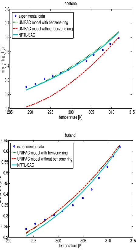
For the NRTL-SAC model prediction, we need to find the four segment numbers for the chemical compound, and then use the segment values to predict the solubility of the compound in other solvents. We selected 1-butanol and acetone for parameter estimation and optimized the values of segment numbers which are shown in Table 2-4.

Table 2-4. Optimized segment numbers for the model compounds using the NRTL-SAC method

Component X (Hydrophobic) Y- (Polar attractive) Y+ (Polar repulsive) Z (Hydrophilic)

3-pentadecylphenol 0.674 0.000 0.571 0.398

Lovastatin 1.175 0.000 0.548 0.882

Valsartan 0.000 0.946 0.000 0.539

20 30 40 50 60 70 80 90 100 110 120 -8 -6 -4 -2 0 2 4 temperature [oC] H e a t fl o w [ m w ], e n d o i s t o t h e t o p

5 10 15 20 25 30 35 40 0 2000 4000 6000 8000 10000 2 Theta in te n s it y

(56)

33

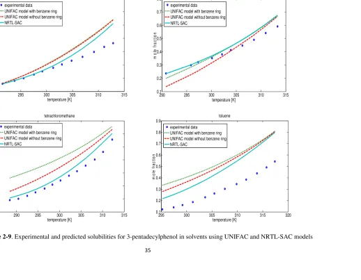
Using the obtained segment numbers for the compound, the NRTL-SAC model predicted solubility in other solvents (Figures 2-9 and 2-10). It can be seen from the results that except for toluene, the solubility in other three solvents were predicted satisfactorily. For all of the four solvents, the NRTL-SAC model resulted in better prediction compared to the UNIFAC. As it is evident from Table 2-5 the polar attractive segment is zero, which implies the molecule has a repulsive nature against polar solvent, due to the electron-rich part of benzene ring. As it was mentioned previously, about 84% of the total volume of the molecule is occupied by the alkyl group, and the remaining is the phenolic part. This makes the molecule to have a good interaction with other polar solvents. For non-polar solvents (such as toluene) the interaction is not the same. That is why the prediction for toluene has some deviation from the experimental results.

Table 2-5. Experimental solubility of 3-pentadecylphenol in pure IPA and its mixtures with water (the mean values with their standard deviation)

Temperature [oC]

15 20 25 30 35

Pure IPA 0.7072 ± 0.0631 0.9436 ± 0.0804 1.4109 ± 0.1233 2.2355 ± 0.1011 3.8502 ± 0.4150 80vol.% IPA 0.7635 ± 0.0659 0.9755 ± 0.1213 1.6026 ± 0.1519 2.3653 ± 0.2608 4.4036 ± 0.2307 50vol.% IPA 0.2302 ± 0.0286 0.3980 ± 0.0419 0.6704 ± 0.0681 1.2739 ± 0.1396 3.1857 ± 0.2867 20vol.% IPA 0.0152 ± 0.0040 0.0188 ± 0.0031 0.0235 ± 0.0045 0.0273 ± 0.0028 0.0329 ± 0.0037

(57)

34

Figure 2-8. Experimental points of the solubility of 3-pentadecylphenol in two solvents and their curve of estimation using NRTL-SAC model. The curves of UNFAC are also shown here for

comparison

285 290 295 300 305 310 315

0.1 0.2 0.3 0.4 0.5 0.6 0.7 0.8

temperature [K]

m

o

le

f

ra

c

ti

o

n

acetone

experimental data

UNIFAC model with benzene ring UNIFAC model without benzene ring NRTL-SAC

290 295 300 305 310 315

0.2 0.25 0.3 0.35 0.4 0.45 0.5 0.55 0.6 0.65

temperature [K]

m

o

le

f

ra

c

ti

o

n

butanol

experimental data

(58)

35

Figure 2-9. Experimental and predicted solubilities for 3-pentadecylphenol in solvents using UNIFAC and NRTL-SAC models

290 295 300 305 310 315

0.1 0.2 0.3 0.4 0.5 0.6 0.7 0.8 temperature [K] m o le f ra c ti o n ethanol experimental data

290 295 300 305 310 315

0.1 0.2 0.3 0.4 0.5 0.6 0.7 0.8 temperature [K] m o le f ra c ti o n ethyl acetate experimental data

2850 290 295 300 305 310 315

0.1 0.2 0.3 0.4 0.5 0.6 0.7 temperature [K] m o le f ra c ti o n tetrachloromethane experimental data

295 300 305 310 315 320

0.1 0.2 0.3 0.4 0.5 0.6 0.7 0.8 0.9 temperature [K] m o le f ra c ti o n toluene experimental data

Pharmaceutical Process Modeling, Optimization, and Control

Scholarship@Western

Scholarship@Western

Pharmaceutical Process Modeling, Optimization, and Control

Pharmaceutical Process Modeling, Optimization, and Control

Pharmaceutical Process Modeling, Optimization, and

Control

Ehsan Sheikholeslamzadeh

Abstract

Acknowledgments

Table of Contents

List of Tables

List of Figures

Chapter 1

Chapter 2

Solubility Measurement and Prediction of Pharmaceutical and

Chemical Compounds in Pure and Mixed Solvents