Numerical Simulation of an Open Channel Ultraviolet Waste-water Disinfection Reactor

(1)

Scholarship@Western

Electronic Thesis and Dissertation Repository

8-15-2013 12:00 AM

Numerical Simulation of an Open Channel Ultraviolet Waste-water

Disinfection Reactor

Rajib Kumar Saha

The University of Western Ontario

Supervisor Dr. Chao Zhang

The University of Western Ontario Joint Supervisor Dr. Madhumita Ray

The University of Western Ontario

Graduate Program in Mechanical and Materials Engineering

A thesis submitted in partial fulfillment of the requirements for the degree in Master of Engineering Science

Follow this and additional works at: https://ir.lib.uwo.ca/etd

Part of the Applied Mechanics Commons, and the Computer-Aided Engineering and Design Commons

Recommended Citation Recommended Citation

Saha, Rajib Kumar, "Numerical Simulation of an Open Channel Ultraviolet Waste-water Disinfection Reactor" (2013). Electronic Thesis and Dissertation Repository. 1450.

https://ir.lib.uwo.ca/etd/1450

This Dissertation/Thesis is brought to you for free and open access by Scholarship@Western. It has been accepted for inclusion in Electronic Thesis and Dissertation Repository by an authorized administrator of

(2)

(Thesis format: Monograph)

by

Rajib Kumar Saha

Graduate Program in Mechanical and Materials Engineering

A thesis submitted in partial fulfillment of the requirements for the degree of

Master of Engineering Science

The School of Graduate and Postdoctoral Studies The University of Western Ontario

London, Ontario, Canada

(3)

ii

Abstract

The disinfection characteristics of an open channel ultra-violet (UV) wastewater disinfection reactor are investigated using a computational fluid dynamics (CFD) model. The model is based on the volume of fluid method to capture the water-air interface, the Lagrangian particle tracking method to determine the microbial particle trajectory and the discrete ordinate model to calculate the UV intensity field. The numerical predictions are compared with the available experimental data to validate the CFD model. A parametric study is performed to understand the effects of different parameters on the disinfection performance of the reactor. The hydraulic behaviour and the additive nature of disinfection for an open channel reactor with two lamp banks placed in series using different geometric configurations between the two lamp banks are also investigated. A scaling down methodology for the open channel reactor is developed and implemented in the CFD model to understand its applicability.

Keywords

(4)

iii

Acknowledgments

I want to thank both of my supervisors for their continuous support and guidance. I would also like to thank Dr. Botao Peng from Trojan Technologies, Inc. London, ON, Canada for his help during the initial stage of this project. This research would have been impossible to finish without the computational resources provided by SHARCNET and the facilities at Western University. Support provided by the NSERC through the ENGAGE program is also acknowledged.

(5)

iv

List of Figures

Figure 1.1: (a) Closed channel UV reactor (b) Open channel UV reactor ... 3

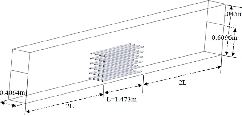
Figure 3.1: Schematic of the computational domain without lamp support system ... 22

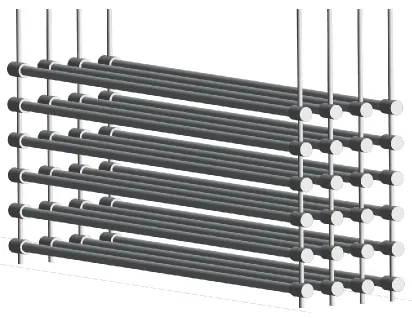
Figure 3.2 Simplified lamp support system ... 23

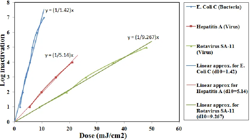
Figure 3.3: Dose-response relationship for some microbes and their approximation to linear kinetics. ... 32

Figure 3.4: Boundary conditions for the momentum and continuity equations ... 34

Figure 3.5: Element distribution at a lateral cut-plane for the geometry without the lamp support system ... 38

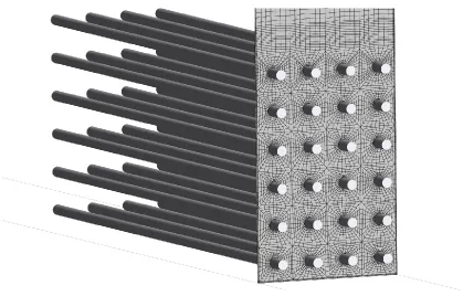
Figure 3.6 The surface mesh on the lamp support and the volume mesh at a lateral-cut-plane. ... 39

Figure 4.1 Free surface profile for the reactor without the lamp support ... 48

Figure 4.2 Free surface for the reactor with the lamp support ... 48

Figure 4.3 Comparison of the predicted normalized water level using different grid sizes for the reactor without the lamp support ... 49

Figure 4.4 Comparison of the predicted normalized water level using different grid sizes for the reactor with the lamp support... 50

Figure 4.5 Comparison of the predicted normalized free surface height with the experimental data. ... 51

Figure 4.6 Log removal of the microorganism for both of the reactor models with and

without the lamp support system ... 52

(9)

viii

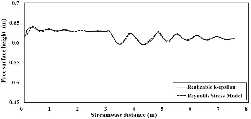
Figure 4.8 Free surface height predicted by and RSM turbulence model ... 54

Figure 4.9 Iso-lines of stream-wise velocity magnitude at 0.5 m upstream of the lamp bank 55

Figure 4.10 Wall shear stress at 0.5m upstream of lamp bank ... 56

Figure 4.11 Comparison of the absolute free surface heights at different flow rates. ... 58

Figure 4.12 Comparison of the pressure head losses within the reactor at different flow rates. ... 58

Figure 4.13 Log removal and the obtainable RED at different flow rates. ... 60

Figure 4.14 Probability density function of UV dose ... 60

Figure 4.15 Stream-wise velocity profile at the mid stream-wise cross section passing

through the lamp ... 61

Figure 4.16 Variation of achievable log-removal with water UVT ... 62

Figure 4.17 UV intensity distribution around the lamps along a horizontal line for different UVT values. ... 63

Figure 4.18 Low dosed particle trajectories colored by the dose value (ranging from 0 to 30 ... 64

Figure 4.19 Stream-wise velocity and turbulence intensity at mid-stream-wise plane ... 66

Figure 4.20 Free surface profile for the two-bank reactor having straight joint (colored with velocity magnitude m/s) ... 67

Figure 4.21 Free surface profile for the two-bank reactor having expanded joint (colored with velocity magnitude m/s) ... 67

(10)

ix

Figure 4.23 Comparison of the free surface heights for the two-bank reactors having different joints ... 69

Figure 4.24 Energy-depth curve ... 71

Figure 4.25 Reduction equivalent dose (RED) for the two-bank reactors compared with the one-bank reactor at 4320 gpm... 72

Figure 4.26 Comparison of free surface profile for the full size and scaled down systems ... 74

Figure 4.27 Probability density of particle residence time at full size and scaled down

models. ... 74

Figure 4.28 Comparison of the disinfection performance between the full size (4320 gpm) and scaled down models using only the Froude number and both Reynolds & Froude

numbers ... 76

(11)

x

List of Tables

(12)

xi

Nomenclature

Absorption coefficient of the

medium Length scale (m)

UV sensitivity of the microbes

Number of potent microbes after and before exposure to UV respectively

Model constants Pressure (Pa)

Drag force coefficient of the

particle Probability density of dose (-)

Diameter (m) Position vector

Dose _{Relative Reynolds number}

Required amount of dose for 1

log removal Direction vector for the RTE

Froude number The scattering direction vector

Body force on fluid element

(N)

Scattering coefficient of the medium

Gravitational acceleration

vector Scalar measure of the _{deformation tensor}

Production of turbulent kinetic energy due to the mean

velocity gradients

Time (s)

UV radiation intensity

Velocity vector (m/s)

Turbulent kinetic energy

(13)

xii

Greek letters

α Volume fraction , Turbulent Prandtl number for

and respectively Turbulent kinetic energy

dissipation rate Fluid stress tensor

Viscosity _{Reynolds stress tensor}

Density

Subscripts

m Molecular t Turbulent

p Particle w Water phase

r Ratio (model to prototype) x x coordinate direction component

s Scattering radiation component

Abbreviations:

CFD Computational Fluid Dynamics RNG Renormalized group theory

DO Discrete Ordinate RSM Reynolds stress model

DRW Discrete random walk RTE Radiative Transfer Equation

LDA Laser Doppler anemometry RED Reduction Equivalent Dose

LDV Laser Doppler velocimetry TKE Turbulent kinetic energy

LSI Line source integration UV Ultra-Violet

MPSS Multiple points source summation

UVT Ultraviolet Transmittance

MSSS Multiple segment source summation

UDF User Defined Functions

PDF Probability Density Function VOF Volume of Fluid

(14)

Chapter 1

1 Introduction

Ultraviolet (UV) light has been used extensively for disinfecting both drinking and waste-water containing microbial species. For waste-waste-water disinfection, UV light is used at the tertiary stage of disinfection. In the primary and secondary stages of treatment, heavy solids and suspended biological components are removed using mainly mechanical processes. Unlike chlorination and ozonation which are commonly used during the tertiary stage of waste-water treatment, ultraviolet light is a green technology as no hazardous oxidation by-products are produced (Oppenheimer et al., 1997). It is also an effective disinfectant for some pathogens like spore forming Cryptospordium and

Giardia lamblia, which are relatively resistant to chemical disinfection (Linden et al., 2002).

The UV light disinfects the microorganism such as bacteria, viruses and pathogens by destroying their nucleic acid (DNA and RNA). This photochemical inactivation process is called dimerization. The UV light promotes a bond formation between nucleotides (thymine-thymine, thymine-cytosine, uracil-uracil and cytosine-cytosine) of two adjacent DNA/RNA strands. This bonding (dimer) prevents the organism from replicating or reproducing. As a result, they cannot infect their host.

1.1 UV Light and UV Lamp Types

In the electromagnetic radiation spectrum UV falls between X-rays and visible light (100 to 400 nm). According to the wavelength it can be classified to following categories:

a) Vacuum UV (100 to 200 nm) b) UVC (200 to 280 nm)

c) UVB (280 to 315 nm) d) UVA (315 to 400 nm)

(15)

a small amount of mercury. The gas is excited with very high voltage difference between the tungsten electrodes. The mercury vapor at higher energy state caused by the arc comes to a low energy state and releases UV light. The wavelength of the emitted UV light depends on the gas pressure inside the lamp. The low pressure (0.93 Pa) lamp only emit light at certain wavelengths, usually 254 nm and 185 nm, (Wright and Cairns, 1998).

The UV absorption and consequently the microbial inactivation vary as a function of the wavelength of UV light. For most microorganisms, the UV absorption by the DNA is the maximum at or near 260 nm and drops to zero near 300 nm (USEPA, 2006). Since the 254 nm output of a low pressure lamp coincides well with this inactivation peak near 260 nm, the low pressure lamp is widely used in disinfections.

Medium pressure (13 kPa) lamps exhibit a continuous spectrum with several peaks. Mostly UVC and UVB are produced. Although in practical applications both the medium and low pressure lamps are used, the low pressure UV lamp is considered in this study.

1.2 UV Reactor Configurations

(16)

Figure 1.1: (a) Closed channel UV reactor (b) Open channel UV reactor

According to the arrangement of the UV lamps, open channel reactors are divided into two types: 1) horizontal configuration where the lamps are placed horizontally, parallel to the flow direction and 2) vertical configuration where the lamps are placed vertically, perpendicular to the flow. The lamp configuration in a reactor affects its disinfection performance. The horizontal configuration has a comparative advantage over the vertical one in terms of the distributed UV-radiation dose. Since the lamps are aligned with the stream-wise direction of the water flow, the exposure time of any microbial particle to the UV light is better in the reactor having horizontal arrangement of the lamps. In the vertical configuration, the lamps may be overheated at the top if the water surface falls below suddenly. This increases the risk of the lamp breakage due to the temperature variations. In addition, several studies were conducted on the open channel UV reactors with vertical configuration, whereas, no studies have been reported on the reactors with horizontal configuration. Therefore, the horizontal lamp configuration is considered in this study.

1.3 Reactor Performance Assessment and the Need for

CFD

Before the UV disinfection reactor can be put to operation its inactivation performance should be evaluated. Quantification of the inactivation credit of a reactor is also important to improve the dose distribution and eventually minimize the energy consumption of the reactor.

(17)

Theoretically the plug flow reactors would provide the best disinfection performance. However, in reality the reactor dose delivery is not uniform. The geometric configuration of the reactor and the exponential decay of the UV intensity field due to absorption in radiation are responsible for the non-uniformity of the dose distribution. In open channel reactors, the waviness at the water-air interface is also responsible for this deviation.

The steps involved in the standard procedure for disinfection performance assessment of a UV reactor are explained in details in USEPA (2006) guideline. The widely used technique is bio-dosimetry, where the inactivation of the challenge microorganism is directly calculated by passing it through the reactor and sampling the inactivation at the outlet. This achieved inactivation is matched with the microorganism's dose response curve. Dose response curve quantifies the inactivation with response to dosage and is found from collimated beam experiments. From this curve the overall dose delivered by the reactor can be calculated from the achieved inactivation. However, if the challenge microorganism's dose-response behavior is not the same as those target organisms, this method cannot predict accurate disinfection behavior. Moreover, bio-dosimetry does not provide any information regarding the local disinfection behavior within the reactor.

If the dose distribution of the reactor could be directly measured by some means, the inactivation from the reactor for a microorganism having any dose-response curve could be easily evaluated. To achieve that purpose, different experimental techniques such as biological dosimeter (Cabaj and Sommer, 2000), Lagrangian actinometry (Bohrerova et al., 2005; Blatchley et al., 2006) and optical diagnostic techniques (Elyasi and Taghipour, 2011; Gandhi et al., 2012) have been developed. However, these experimental techniques require full size reactor model, which may not be cost effective for investigating multiple designs. One alternative approach is the use of numerical techniques to resolve the hydraulics and optics occurring inside the reactor and to calculate the dose distribution from that.

(18)

modifications. Most of the computational studies performed to date on the UV disinfection reactors are restricted to closed channel configuration. However, the open channel configuration is widely used in wastewater treatment plants. Due to the complicated flow characteristics arising from the free surface in an open channel configuration, a comprehensive investigation is necessary. Literature provided a few instances of the simulation of the vertical type open channel reactors, whereas, none was found on the horizontal type. However, these works were based on different simplification, such as two-dimensional assumption and simplified turbulence models. These simplifications limited the applicability of these models to general reactor configurations. For example, the two-dimensional depth averaged model does not take into account of the free surface in an open channel reactor. Therefore, its effect on the hydraulics and disinfection process is not accounted for. The width averaged two-dimensional model would provide inaccurate results as it neglects effects coming from the side walls. As the disinfection characteristics of the reactor is dependent on turbulent mixing within the reactor, two-dimensional model neglects the three-dimensional effect of turbulence and any secondary flow features that are governed by turbulence. Moreover, in a two-dimensional approximation, the cylindrical shape of the lamp cannot be properly accounted for. For this reason the USEPA guideline also suggests that for investigating the reactor performance a three-dimensional model should be considered.

However, three-dimensional simulation is computationally expensive if all the geometrical details of the reactor are included in the simulation. A balance between the accuracy and the computational cost needs to be considered. For this reason the geometry of the reactor needs to be simplified, for example the cleaning system and the inlet and outlet reservoir can be removed to reduce the computational cost, and a simplified lamp support system or without the support can be used. Once validated, the simplified geometry would be used for analyzing different configurations of the lamp banks and other parametric studies.

1.4 Objectives of this Work

(19)

horizontally arranged UV lamps. Then, a parametric study of the UV reactor is performed using the proposed CFD model to understand the effects of operating parameters such as water flow rate and UV transmittance (UVT). The effect of UV sensitivity of the microbes to be treated on the disinfection performance of the reactor is also investigated.

In wastewater treatment plants, the lamp banks can be placed in series within the open channel to increase the inactivation. The geometric parameters, such as channel constriction/expansion between the lamp banks, can affect the additive nature of the dose delivered. The proposed CFD model is also used to investigate the effect of the geometric parameters on the hydrodynamic and disinfection behavior of the reactors with particular attention to the additive behavior of the delivered dose.

Due to the size of the open channel UV disinfection systems, evaluating their performance experimentally at the design stage is not economically feasible, especially for design optimizations. A small scale reactor which can predict the behavior of the large scale system, would be highly beneficial, to experimentally verify the proposed design. However, due to the interaction of hydraulics, optics and microbial inactivation kinetics, scaling down the UV reactor may be complicated. A scaling methodology for both hydraulics and the disinfection characteristics needs to be formulated. One way to verify the developed methodology is to implement that numerically through the developed CFD model. The disinfection characteristics of the full size and the scaled down reactors predicted by the CFD model can be compared to verify the validity of the developed scaling methodology. Therefore, another objective of this work is to investigate the scalability of the UV disinfection reactor through CFD simulations.

In summary the objectives of this work are:

1. To establish a three-dimensional CFD model that is capable of predicting the disinfection performance of the UV reactor.

2. To perform a parametric analysis to understand the effect of different operation parameters on the disinfection performance.

(20)

4. To investigate the possibility of having a small scale model to predict the performance of a full size system.

1.5 Outline of the Thesis

This thesis is organized in five chapters. A brief description of the topics discussed in the following chapters is provided below:

 Chapter 2-Literature Review

 This chapter provides a detail discussion of the previous research works relevant to the current study.

 Chapter 3-Description of the Numerical Model

 In this chapter, a comprehensive description is provided for the developed numerical model. The boundary conditions and the numerical solution techniques are discussed. The detail descriptions of the reactor geometry and grid generation are provided. At last the scaling down methodologies for both the hydraulics and the optics are explained in detail.

 Chapter 4-Results and Discussion

 The grid sensitivity analysis is performed first and then the model is validated against the available experimental data. Then, the validated model is used to investigate the hydraulic and disinfection behavior of the reactor under different flow conditions and geometric parameters. The effects of optical characteristics of the water and the UV sensitivity of different microbes on the disinfection performance are also discussed. At last the validity of the developed scaling down methodology is discussed by comparing the hydrodynamic and the disinfection behavior of the full size and 10 times scaled down reactor.

 Chapter 5-Conclusions

(21)

Chapter 2

2 Literature Review

In this chapter a comprehensive literature review is presented on the numerical simulation of UV disinfection reactors. A majority of the previous studies were performed on the closed channel UV reactors and a few were reported on the reactors having open channel configuration. To understand the effect of different aspects of the computational model, studies on both of these reactor types are discussed.

A gap in the literature is identified in terms of the free surface tracking schemes and the comparative advantages/disadvantages of different turbulence models in the open channel UV disinfection reactors. This gap has arisen because all the previous works in this field were based on two-dimensional depth averaged models and the effects of the free surface were neglected.

2.1 Application of Different Computational Models in UV

Reactor Simulations

(22)

investigated. In this section different studies are reported in a chronological order in an attempt to elucidate the advantages and shortcoming of these above mentioned aspects of the computational model.

One of the earliest attempts to simulate the UV disinfection reactor was accomplished by Downey et al. (1998). They used a computational fluid dynamics model composed of Reynolds averaged Navier-stokes equation and the standard turbulence model to simulate the liquid flow in a closed channel reactor. The microorganism particle trajectory was calculated in a Lagrangian frame of reference. The residence time of those particles in the reactor outlet was compared with that achieved from the salt tracer test experiment. They reported that at lower flow rates the predicted residence time distribution was within 95% confidence interval with reference to the experimental values. However at higher flow rates the predicted residence time was underestimated. The study was only limited to the calculation of the flow field inside the reactor. The model did not include the calculation of the UV intensity field and consequently the dosage delivered by the reactor was not calculated.

The first study reported in the literature on the simulation of an open channel UV reactor was the work by Lyn et al. (1999). They used a steady two-dimensional depth averaged model to predict the turbulent flow in a vertical type open channel UV reactor. Since the depth averaged two-dimensional model was used, the effect of the free surface was not accounted for. The flow model was based on Reynolds averaged Navier-Stokes equation and the turbulence model. The predicted velocity was compared with Laser Doppler anemometry (LDA) data. They reported good agreement in the velocity field at the upstream of the channel. However, at the wake region of the lamps, the predicted flow field showed some deviations compared to the experimental measurements. The UV intensity field was calculated using the point source summation (PSS) technique and the disinfection was modeled in an Eulerian framework. They reported that at higher flow rates the disinfection prediction was satisfactory, however, deteriorated at low flow rates.

(23)

found from a model that combined the velocity field obtained from experimental measurements using Laser Doppler velocimetry, the particle trajectory information from a Discrete Random Walk (DRW) model based on the measured velocity field and the UV intensity field from a PSS model. The exit dose for the microorganism particles was calculated by performing a time integration of the radiation intensity along their trajectories within the reactor. They found that tracking around 10,000 particles can provide an accurate representation of the dose distribution when using the DRW model. The exit dose distribution calculated from this model matched quite well with the experimental disinfection data from a pilot scale vertical type open channel UV reactor. They hypothesized that this disinfection tracking on a Lagrangian framework can accurately represent the physics of the overall disinfection process. However, the effort and time necessary to obtain the turbulent velocity field experimentally was a limitation to this approach. Therefore, they suggested the use of computational fluid dynamics to resolve the flow field variables.

In a continuation work, Chiu et al. (1999b) considered some design modifications to improve the disinfection performance of the vertical type open channel UV reactor. In the previous study, they noticed that there exist some critical paths for the microorganism particles, which leads to the poor performance of the disinfection process. These paths are from the regions away from the lamps where the UV intensity is low and the fluid velocity is high, therefore, dosage they received is low. To mitigate this problem, they modified the reactor geometry by placing waviness and baffles on the channel walls. The disinfection from these modified systems had improvements over the original one. Their developed model showed good agreement with the experimental data at the medium to high velocities. However, at a lower velocity, they noticed some deviation in the numerical predictions of the disinfection. They attributed this deviation to the inherent inaccuracy in the dose-response kinetic model used to represent the microorganism.

(24)

between the results obtained from these turbulence models. The Reynolds stress model predicted slightly different turbulent kinetic energy. However, this difference had little effect on the velocity and consequently disinfection prediction. They concluded that the use of standard model was sufficiently accurate for disinfection prediction.

(25)

Lyn (2004) used the standard turbulence model to simulate the open channel UV disinfection reactor having vertical arrangement of the lamps. They used a two-dimensional depth averaged computational model. This study was mainly focused on evaluating the effect of unsteadiness due to the vortex shedding from the vertical lamp array on the prediction of the dosage distribution in the reactor. They compared the time averaged unsteady solution with the solution found from a steady state analysis. They found that the difference in the prediction between the time-averaged and the steady state solution was higher in the entrance region of the vertical lamp array and lower in the downstream. They compared these results with the experimental data and found that the time-averaged unsteady model prediction was in better agreement. However, the turbulent kinetic energy was underpredicted in both of these models. Lyn and Blatchley (2005) used the same two-dimensional CFD model for an open-channel vertical type UV system and compared the Lagrangian approach to the Eulerian approach to track the disinfection in the reactor and found similar results in the inactivation of the microorganisms.

Ducoste et al. (2005) used the RNG model to simulate a closed channel UV reactor. They used both the modified LSI model and the MPSS model based commercial code UVcalc3D to calculate the UV intensity field. This study was also mainly focused on evaluating the Eulerian and Lagrangian methods for the disinfection tracking. In the Eulerian method, they calculated the fluence distribution using a flow-weighted and a mass-weighted fraction technique. They mentioned that the fluence distribution calculated by the Lagrangian technique was not sensitive to the size of the particles used to represent the microorganisms, the wall restitution coefficient for particle reflection or the time step resolution used to capture the particle trajectory. They found that the disinfection predicted by both the Eulerian and the Lagrangian methods provided very good match at the reactor outlet and showed reasonable agreement with the experimental bioassay tests. They concluded that both of these methods can be used alternatively for tracking the disinfection in an UV reactor.

(26)

of the inlet and outlet ports. This work was also focused on comparing different computational techniques (Lagrangian vs. Eulerian) for calculating the dosage distribution inside the reactor. They used the LSI and the MPSS model to capture the UV intensity field inside the reactor. Predicted dose distributions from both the Lagrangian and Eulerian model showed very good agreement with each other at higher flow rates, however, exhibited slight discrepancy at lower flow rates. The computed dose distribution showed very good agreement with the bio-dosimetry data obtained from an industrial prototype UV reactor.

Elyasi and Taghipour (2006) simulated a close channel annular UV reactor. They used the realizable model for resolving the turbulence. The disinfection was tracked in an Eulerian framework. Based on the model that they validated, they suggested that the Eulerian approach of disinfection tracking has some advantages over the Lagrangian approach. As an example, they showed that the local volumetric rate of inactivation can be better captured by the Eulerian approach, thus providing insight for better reactor design.

Pan and Orava (2007) evaluated disinfection performance of a closed channel UV reactor for different geometric and flow configurations. They used the standard turbulence model at the core flow region and an algebraic model at the boundary layer region. They used the MPSS model to resolve the UV intensity and an Eulerian approach to calculate the disinfection performance.

They mentioned that the accurate prediction of the UV intensity is dependent on the efficiency of the lamp, quartz transmittance and the extent of reflection at the walls. However, the uncertainties associated with these variables have less influence on the accurate calculation of the disinfection efficiency of the reactor. They concluded that the reactor's disinfection performance/accuracy is mainly dictated by the flow conditions and the orientation of the lamps inside the reactor, which can produce wide differences in the disinfection performance.

(27)

two-fluid model (TFM) to resolve the flow field in a closed conduit UV reactor. They validated the predicted velocity values and the turbulent kinetic energy with experimental data obtained using the digital particle image velocimetry (DPIV). They found that both the standard and RNG models exhibited fairly good match with the experiments in predicting the velocity field at different locations inside the reactor. The RSTM exhibited better match in the velocity field. In predicting the turbulent kinetic energy, the model showed greater deviation from the experimental measurements. They pointed out that the discrepancies between the predicted velocity and turbulence field were mainly in the wake region of the lamps. They used the MSSS model to calculate the UV intensity field and a Lagrangian particle tracking approach to calculate the dosage on the microorganism particles. Their results showed that the dosage distribution and consequently the inactivation rate were sensitive to the turbulence model selected. For example, turbulence models which predicted larger wake region behind the UV lamps exhibited a broader dosage distribution. The sensitivity of the microorganism was also a contributing factor to these deviations. The microorganisms having a higher UV sensitivity showed greater sensitivity to the turbulence model selection.

Munoz et al. (2007) used a three-dimensional CFD model to predict the performance of a full-scale closed channel UV reactor for disinfection of drinking water. They used both

the model and the RSM to resolve the turbulence field. The predicted velocity and

turbulence variables from these two models were almost the same. The difference between the predicted reduction equivalent doses among these models was less than 4%, thereby suggesting that the effect of turbulence model was not prominent in calculating the disinfection. They used the Lagrangian particle tracking with the Discrete Random Walk (DRW) model to resolve the microorganism trajectory. To resolve the UV intensity field, the commercial code UVCalc3D, which is based on MSSS, was used. They developed an approach to investigate the sensitivity of number of Lagrangian particles used in DRW model for calculating the dose distribution. They found that around 30,000 particles can provide insensitive results. The Lagrangian time constant of 0.15 for the

model and 0.3 for the RSM provide reasonably accurate result when DRW is used.

(28)

unstructured hexahedral mesh with same level of resolution. Based on that, it was suggested that the unstructured tetrahedral mesh should be used in caution. The effect of unsteadiness in the flow field on the calculated disinfection was also evaluated. They found that the computed inactivation and the reduction equivalent dose in the unsteady model varied less than 2% compared to the steady model. Based on this finding, they suggested that the steady state model is adequate for the disinfection prediction.

Wols et al. (2010) simulated a UV bench-scale reactor using a CFD model and validated with experimental techniques. They used salt particles to measure the residence time distribution, dye injection to visualize the mixing patterns and LDA measurement to calculate the local velocity profile. The CFD model comprised of the standard turbulence model, MPSS for fluence field calculation and Lagrangian particle tracking for disinfection calculation. They found that the velocity field has good comparison with the experimental data, however, failed to capture the recirculation region, especially at the wake of the lamps. They also reported that the CFD model predicted higher mixing rate compared to experimental measurements resulting in a narrower residence time distribution.

(29)

2.2 Application of Free Surface Tracking Schemes and

Turbulence Models in Open Channel Flow Simulation

It is evident from the above section that all the simulations on the open channel reactors performed so far adopted the depth averaged two-dimensional representation of the reactor. Therefore, the water-air interface tracking technique has remained un-discussed. Since a three-dimensional model is used in this study to incorporate the effect of the free surface, the vast area of the open channel flow simulation is briefly discussed in this section to find out the available and mostly used models to track the water-air interface.

Tracking a free surface in a numerical simulation includes an extra difficulty to the computational model. Usually there are two approaches to tackle this problem, the first one tracks the interface in a Lagrangian fashion and the second one uses a fixed Eulerian mesh and solves a transport equation for the volumes of the individual fluids forming the interface.

The first method (i.e. Lagrangian interface tracking) can accurately capture the deformable interface by moving the mesh nodes at those points at a velocity equal to the normal local fluid velocity. However, cases which include large movement of the interface, the mesh deteriorates seriously at those points. To prevent that, the Arbitrary Lagrangian Eulerian (ALE) method was introduced. Literatures provided few instances of using this method in the application of open channel flow (Srinivas, 1992; Ming-Hsi et al., 2001). This approach was not adopted in open channel flow simulations, mainly because of the associated higher computational cost. However, this method has reserved its applications for the fluid-structure interaction problems.

(30)

Abbaspour et al. (2009) used the VOF method to study the hydraulic jump (increase in free surface height) after a sluice gate. They used a two-dimensional approximation with the standard and RNG turbulence models. They have shown that the VOF method can accurately capture the rise in water-air interface and the predicted free surface values were within a range of 1-8.6% of experimental measurements.

Patil et al. (2009) simulated the open channel flow over bridge decks on different flooding conditions. They used the transient implementation of the VOF to capture the free surface and the RNG for the turbulence. They have mentioned that the transient VOF is sensitive to the computational input parameters and showed slight deviation from the limited experimental data.

Akoz et al. (2009) compared the experimental values of velocity and free surface profiles along a sluice gate with the computational ones. They showed that both the free surface and the velocity profile were accurately predicted by the computational model, which used the VOF method for interface tracking and the model for turbulence.

Cassan and Belaud (2012) studied the flow characteristics in the upstream and downstream of a sluice gate. The two-dimensional computational model was composed of VOF method for free surface tracking, RNG model and RSM for turbulence. They found very good agreement in the predicted velocity profile and head loss in the sluice gate, when compared to the experimental values.

Considering these successful applications of the VOF model in open channel flow simulations and the associated low computational cost, this approach is adopted in this study to capture the water-air interface in the open channel UV reactor.

(31)

Within the Reynolds averaged Navier-Stokes approaches, the two equation turbulence model and its different variations have been applied extensively for open channel flow simulations (Sinha et al., 1998; Wu et al., 2000; Smolentsev et al., 2002; Ma et al., 2002; Rameshwaran and Naden, 2003; Nezu and Sanjou, 2006; Jha and Bombardelli, 2009; Patil et al., 2009) These two equation models assume the isotropy in turbulence through the Boussinesq approximation. However, this approximation is not always valid in open channel flows. For example, in straight open channels having rectangular cross section, there might exist a secondary flow feature, which is produced only due to the anisotropy in turbulence (Nezu et al., 1993). Since the turbulence model assumes isotropic turbulence, it cannot capture these behaviours. To account for the anisotropy in the turbulence field, some researchers have used the algebraic stress model (ASM), which is economical in terms of the computational cost (Demuren and Rodi, 1984; Sugiyama et al., 2006; Cea et al., 2007). However, since the ASM does not solve the exact equations for Reynolds stresses, rather uses empirical relationships, the accuracy of the model prediction is highly problem dependent. To overcome this issue, the Reynolds stress turbulence model has been successfully used by different researchers (Kang and Choi, 2006; Jing et al., 2009).

2.3 Conclusion

After investigating the aforementioned studies on both UV reactors and general open channel flow simulations, both and the RSM turbulence models are adopted in this study to capture the detail turbulent flow characteristics inside the reactor.

The unsteadiness due to the vortex shedding from the lamps, as pointed out by Younis and Yang (2011), was for a reactor having vertical arrangement of the lamps. In this study the lamps are placed parallel to the stream-wise direction. Thus, this effect can be ignored. Based on the findings of Munoz et al. (2007), the steady state approximation led to very similar results in comparison to the time averaged unsteady simulation. Therefore, a steady state approximation is adopted in this study to reduce the computational effort.

(32)

intensity near the lamps. They suggested that this discrepancy is due to the negligence of the refraction effect at the lamp quartz sleeve. Bolton (2000) found that for water samples with higher UVT (equal or more that 70%) significant error (up to 25%) arises in the calculated UV intensity field if the effect of refraction is neglected. Since Liu et al. used water samples with ultraviolet transmittance (UVTs) values of 77 and 88 [%/cm], their finding goes well with Bolton's finding. Bolton also suggested that in most wastewater applications where the UV disinfection is used, the UV transmittance values are usually much less than 70%. Thus, discarding the refraction causes only a minor error. Since the UVT of the wastewater in the current study is below 70%, the effect of refraction can be neglected.

Another important point is that the MPSS and MSSS with refraction, reflection and absorption are computationally expensive and could be difficult to deal with while solving for a reactor having multiples lamps. Bolton (2000) showed that the number of point sources should be greater than 1,000 to produce an accurate representation of the UV intensity around the lamp. Therefore, from the computational cost point of view, the DO model is suitable for this study.

All of comparative studies on the Eulerian and Lagrangian approach for the disinfection tracking suggested that both of these approaches produce the results with similar levels of accuracy. Therefore, the Lagrangian approach is chosen as it is more intuitively promising and enables the visualization of the low/high dosed particle trajectory inside the reactor, thus providing insight of the whole disinfection process at a glance.

The VOF model is adopted for this study based on the successful implementation of this model to capture the water-air interface for general open channel flow simulations and considering the associated low computational cost.

(33)

(34)

Chapter 3

3 Description of the Numerical Model

In this chapter, the geometric configuration of the reactor will be presented first. Then, a detailed description will be provided for the numerical model proposed in this study. The boundary conditions and the numerical solution techniques will be discussed. A brief description of the grid generation procedure will be provided along with the snapshot of the grids used in this study. At last the scaling down methodology for both the hydraulics and the optics will be explained in detail.

3.1 The Reactor Geometry

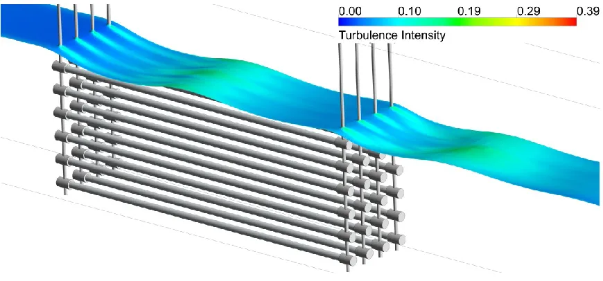
The reactor used in this study is an open channel reactor with one bank of lamps placed inside the reactor horizontally, which is parallel to the main flow. The bank is composed of 24 lamps, 4 in the lateral direction and 6 in the vertical direction. The vertical assembly of 6 lamps are called modules. The lamps are low pressure UV lamps with 92W power rating, which emit nearly monochromatic light at 253.7 nm wavelength. This wavelength is close to the germicidal inactivation peak for E. coli and Cryptosporidum

(Linden et al., 2001). The electrical efficiency of the lamps is assumed to be 100%. It is also assumed that the full lamp power is used for the light emission in the narrow wavelength range of 253 to 255 nm. The effect of fouling on the lamp sleeve surface is ignored.

(35)

surface is controlled using a weir placed at the downstream of the reactor. In this study, the free surface at the outlet is kept at a height of 0.6096 m.

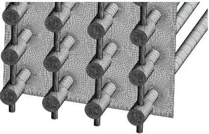
Another geometry used in the simulation includes a simplified lamp support system to investigate the effect of the lamp support system on the numerical results. The close up of the simplified lamp support system is shown in Figure3.2.

(36)

Figure 3.2 Simplified lamp support system

3.2 Computational Model

The computational model is divided into four parts. The first part deals with resolving the flow characteristics in a typical turbulent open channel flow with water-air interface tracking. The second part deals with resolving the trajectories of the microbial particles flowing with the water. The third part is the calculation of the UV intensity field within the reactor. And the final part implements the inactivation kinetics on each microbial particle to calculate the overall log inactivation achievable in the reactor and the reduction equivalent dose (RED) value.

3.2.1 Turbulent Open Channel Flow with Water-air Interface

(37)

turbulent, the Reynolds averaged Navier-Stokes equation is used. The continuity and the momentum equations are given below.

(3.1)

(3.2)

where and are the fluid stress tensor and the Reynolds stress tensor. The physical properties in Eqs. (3.1) and (3.2) are obtained from individual fluid properties based on the mixture rule. For example, the density of the mixture is calculated as following:

(3.3)

where and are the volume fraction and the density of water, respectively. and are the density of the mixture and the air, respectively.

The interface is tracked by solving a transport equation for the volume fraction of the heavier fluid, the water in this case. This is basically a continuity equation for the water phase. The heavier fluid is usually chosen, because satisfying its mass conservation is more important than the lighter fluid. The transport equation is expressed as:

(3.4)

Eq. (3.4) is solved with the constraint that the summation of the volume fraction of water and air should be unity. The air volume fraction is calculated accordingly.

The Reynolds stress tensor in Eq. (3.2) needs to be modeled to close the governing equations. For this purpose the eddy-viscosity concept or the Boussinesq approximation is used. In Boussinesq approximation, the Reynolds stress is expressed in terms of the mean velocity gradients and two new quantities namely, turbulent viscosity and

turbulent kinetic energy . The expression for the Reynolds stress in indicial

(38)

(3.5)

where represent the fluctuating component of the velocity and represents the mean velocity. Subscripts and represent the coordinate directions. The turbulent kinetic energy is the energy per unit mass of the fluid associated with the turbulent fluctuating motion and is defined as:

_(3.6)

To solve for and two additional transport equations are necessary. In this work, the realizable turbulence model is adopted. In this model, the transport equations are solved for the turbulent kinetic energy and its dissipation rate . The equations are as follows:

(3.7)

(3.8)

where is the production of turbulent kinetic energy due to the mean velocity gradients and is a function of , and mean strain rate. is a model constant and is the scalar measure of the deformation tensor. and are the turbulent Prandtl number for and

and assigned constant values, respectively.

The realizable model differs from the standard model in terms of the expression for turbulent viscosity. In the standard model, is calculated using the following formula:

(39)

where is a constant. However, in the realizable model, includes the effect of

mean rotation on the turbulent viscosity and therefore is a function of mean strain and rotation rates, the angular velocity of the system rotation and the turbulence field and (ANSYS FLUENT Theory Guide, 2010).

Turbulence is highly affected by the presence of the walls. Near the walls, the viscous damping reduces the tangential fluctuation and the kinematic blocking reduces the normal fluctuation of the velocity. Due to the sharp velocity gradient in the boundary layer near the wall, turbulence is rapidly generated. Therefore, wall functions, which are semi-empirical correlations, are used to bridge the gap between the viscosity dominated sublayer and the core turbulent region. The main benefit of using a wall function is that a relatively coarse mesh can be used as long as the first cell falls in the logarithmic region of the turbulent boundary layer, i.e. the non-dimensional distance from the wall for the first cell is above 30. The upper limit usually varies according to application (Reynolds number), but in general the value of 200 is considered to provide reasonably accurate result. However, this approach gives erroneous result when the first cell falls in the buffer layer, thus it restricts the grid refinement which is necessary to resolve the whole boundary layer with sufficient number of grid points. Moreover, the near wall effect of turbulence is not well accounted for.

Another approach to resolve the turbulence near the wall is enhanced wall treatment. This approach does not have any stringent requirement for the non-dimensional for the first cell. The blending of the law of the wall for laminar region to the log law region is used in this approach and the turbulent viscosity within the viscous sublayer to the full turbulent region is calculated using a blending function (ANSYS FLUENT Theory Guide, 2010).

(40)

three-dimensional simulations, this model requires 7 additional transport equations to be solved. The transport equations are not listed here and can be found in the ANSYS FLUENT Theory Guide (2010).

3.2.2 Microbial Particle Trajectory

The microbes are modeled as spherical particles having an average of 1 micron diameter. Ducoste et al. (2005) showed that the disinfection predicted by the Lagrangian tracking is not sensitive to the diameter of the particles used. The density of the particles is taken to be same as the density of water, which is based on the fact that most of the microbes have almost or more water content in them. The trajectories of the microbial particles are calculated by integrating the force balance on the particles in a Lagrangian frame of reference. The force balance in the -direction can be expressed as:

(3.10)

where is the particle diameter and is the relative Reynolds number based on

particle diameter and the relative velocity of water and particles. is the drag force coefficient for spherical particles and is expressed as:

(3.11)

where and are constants given by Morsi and Alexander (1972). The Brownian motion of the particles are neglected since the velocity magnitude of the microorganism dictated by the carrying water is significantly high as the flow is turbulent. The force on the particles resulting from the pressure gradient in the flow field is also neglected as it is only important when the fluid density is higher than the particle density.

(41)

the time spent in turbulent motion along a particle path is calculated from the turbulent kinetic energy and its dissipation at every point.

(3.12)

In the DRW model the interaction of a particle with successive fluid phase eddies are included. Each eddy is characterizing by a eddy life time and a Gaussian distribution of the fluctuating velocity.

(3.13)

here, is a normally distributed random number. The characteristic life time of the eddies are calculated from the following

(3.14)

here, is a uniform random number between 0 to 1. The particle is assumed to interact with the fluid phase over the smaller of the eddy lifetime and the eddy crossing time. When this time is reached a new value of the instantaneous velocity is obtained by applying a new value of . By computing the trajectory for a sufficient number of representative particles, the random effects of turbulence on the particle dispersion can be accounted for.

3.2.3 UV Intensity Field

The UV light while propagating from the lamp surface interacts with the medium by four different ways: absorption, reflection, refraction, and scattering. Brief descriptions of these phenomena are given below:

1) Absorption refers to the change in the intensity due to the conversion of the light energy to other forms, while it passes through a medium.

(42)

3) Reflection refers to the change in the direction of the light after hitting a surface, specular/diffuse.

4) Scattering refers to the change in the direction of the light propagation after hitting a suspended particle in the medium.

The effect of absorption and scattering depends on the optical qualities of the water being treated. The UV absorption coefficient and the UV transmittance (UVT) are widely used to characterize them.

The UV Transmittance (UVT) is the percentage of light passing through the medium over a specified distance. The UVT is expressed as following:

(3.15)

where is the UV transmittance _, _{is the Intensity of light transmitted} through the sample _and _{is the Intensity of light incident on the sample}

_. _{is the reduction in intensity over 1 cm.}

The absorption coefficient can be related to the UV transmittance (UVT) by the use of Beer-Lambert's law, which states that the UV intensity decreases exponentially due to the effect of absorption in a homogeneous medium, with zero turbidity (suspended solid particles).

(3.16)

Usually the value of absorption coefficient of water changes over the wavelength spectrum of the UV radiation. However, since a monochromatic UV at 254nm is considered in this study, the value of at this wavelength is considered. The turbidity of the medium is assumed to be zero, since the concentration of solid particles is low in pre-treated effluent prior to UV disinfection.

(43)

_(3.17)

Therefore, if the distance , _{and the absorption} coefficient can be calculated from the UVT as following:

(3.18)

It can be noticed that the absorption coefficient is the slope of the straight line of UV intensity vs. path length plot in a logarithmic scale and the absorption coefficient is in _{, 100 is used to convert} _to _{and the UVT is in the fractional form.}

In this study, the UV intensity field is resolved using the discrete ordinate (DO) model, where the radiative transfer equation (RTE) is solved at every control volume for a finite number of direction vectors (solid angles). The number of RTEs increases with the number of discrete solid angles used. The radiation intensity depends on the spatial coordinates, direction vectors and radiation frequency. However, in this work, the frequency dependence is ignored as the low pressure UV lamps are fairly monochromatic. The RTE for a non-gray radiation is expressed as:

(3.19)

(44)

3.2.4 Inactivation Kinetics

The dose-response relationship of the microbial species is considered to be of the first order, which can be expressed mathematically as:

(3.20)

where is the number of potent microbes at any instant, is the radiation intensity, is the time of exposure and is the sensitivity of the microbes to UV, which is considered to be constant over the entire inactivation. The solution of Eq. (3.20) is:

(3.21)

where, is the number of potent microbes at time zero. The integration of the radiation intensity over time is termed as Dose . In Eq. (3.21), the natural logarithm is changed to 10 based logarithm by correcting the UV sensitivity with a multiplication factor. The following equation is obtained:

(3.22)

It should be noted here that is usually defined as the log removal or log inactivation. In Eq. (3.22), the quantity represents the UV sensitivity of the microbial species, which represents the required amount of dose for 1 log removal. The significance of d10 values is that greater inactivation occurs at lower d10 values for the same applied dosage value on the microbe. This dose-response relationship can be expressed as either the proportion of microorganisms inactivated or the proportion of microorganisms remaining as a function of UV dose applied. Microbial inactivation has a dose-response curve with a positive slope, while microbial survival has a dose-response curve with a negative slope.

(45)

different virus and a bacteria) are shown in Figure 3.3 which follow a linear dose-response relationship based on the data obtained from Chevrefils et al. (2006). The slope of the straight line corresponds to the 1/d10 value mentioned in Eq. (3.22). For the microbes plotted in this figure, the d10 values are ranging from 1 to 10 . However, a wide range of d10 values (1 to 25 ) are considered in this study to cover more microbes, including spore forming bacteria, which are usually difficult to inactivate.

Figure 3.3: Dose-response relationship for some microbes and their approximation to linear kinetics.

In the numerical model, the dose is calculated by the time integral of the radiation intensity over the trajectory of each particle (Chiu et al., 1999a). A custom user defined function (UDF) is developed in the ANSYS FLUENT to obtain the UV dose that a microbial particle is exposed to during its residence time within the reactor. The UDF can be found in Appendix A.

(46)

inactivation rates for different microbial particles. However, an average dose delivered by the reactor needs to be established to quantify its inactivation performance. Therefore, either the survival or inactivation fraction for the microbes has to be averaged over the entire dose range. Based on the average survival/inactivation fraction, the corresponding dose value is calculated from the dose-response relationship of the microbe. This dose value is named as the RED of the reactor. Considering the first order dose-response relationship, the expression for the RED can be mathematically expressed as (Liu, 2004):

(3.23)

where is a weighting function, which accounts for the probability of a microbe getting a dose value of . In the numerical model considered in this study, this represents the number of microbial particles getting dose in a distinct dose interval. The

above integral is evaluated by numerically averaging the survival fractions for all the particles and then calculating the log inactivation from that. It should be noted that the probability of occurrence is taken into account while taking the arithmetic average of survival fractions of all the tracked particles. The higher probability region of dose histogram typically would have more number of tracked particles, thus, the survival fraction or inactivation value in that region gets more weight during summation. To calculate the RED, the corresponding dose value for the average log inactivation is found from the dose-response curve.

(47)

3.3 Boundary Conditions and Numerical Solution

Techniques

In this section, the boundary conditions used for the computational domain shown in Figure 3.1 are summarized. A brief description is also provided on the numerical techniques required to get solutions from the governing equations.

The boundary conditions necessary for the fluid flow equations are summarized in Figure 3.4. To represent the inlet sluice gate, the upper half of the inlet section is specified a no-slip boundary condition and the lower half section is set as a velocity inlet boundary condition corresponding to the mass flow rate of water in the reactor. For turbulence models the wall normal gradient of turbulent kinetic energy is set to zero at walls. The height of the lower half is taken to be the same as the expected free surface height in the reactor, which is 0.6096 m. A uniform velocity profile is assigned since the actual velocity profile at this section is not known. A pressure outlet boundary condition is implemented at the outlet of the reactor. A hydrostatic pressure profile is applied based on the free surface location. The front, back and bottom boundaries are assigned no-slip condition. The top boundary is also considered to be pressure outlet with atmospheric pressure specified there.

(48)

The convergence behaviour of the solution using the multiphase VOF model is sensitive to the initial values used. The volume fraction of water is initialized in the water domain. A hydrostatic pressure based on the depth from the expected free surface height is also initialized.

The discretized form of the transport equation for water volume fraction requires the calculation of the volume fraction flux at a cell face by interpolation from the cell centre values. It was found that the upwind schemes (both second and first order) are highly diffusive, i.e. it results in a diffusive or wider water-air interface. The QUICK scheme was also tried and it provides similar diffusiveness. Therefore, a modified version of high resolution interface tracking scheme (HRIC) is used to solve the transport equation for the volume fraction. The second order upwind discretization is used for all other equations. The least squares cell-based scheme is used to calculate the gradient of the variables.

For the realizable model, the turbulent intensity at the reactor inlet and the hydraulic diameter are specified. Since this is an internal flow, the importance of the value for the turbulent intensity at the inlet is not critical as most of the turbulence is generated internally within the domain due to the shear in the mean velocity field. Considering the Reynolds number based on the hydraulic diameter of the reactor inlet is in the order of , the turbulence intensity at the inlet is specified to be

_{. This expression is based on the turbulence intensity for the fully}

developed pipe flow.

(49)

In the Lagrangian particle tracking model, according to Munoz et al. (2007) the number of particles tracked will affect the accuracy of the calculated dose distribution. The multiplication of the number of particles injected and the number of tries are the actual number of particles tracked. To maintain statistical significance of the particle trajectories and the dose values on those particles, around 75,000 particles are tracked at each simulation (25000 particles with 3 tries).

For the particles, a reflect boundary condition is used at the walls with very low normal reflection coefficient to make sure that the particles do not go far away after hitting a wall boundary. Since the free surface position is not known a priori, applying a boundary condition there for the particles is not possible. However, these particles should stay in the water domain. Although neutrally buoyant particles are used, their velocities are governed by the mixture velocity. Therefore, some particles might go to air region following the mixture velocity field. To enforce the particles to stay in the water, a UDF is used which deletes a particle when it reaches a cell with very low water volume fraction.

For the DO model, it is assumed that all the incident radiations at the reactor walls are absorbed and none is reflected. The emissivity of the wall is set to 1 to implement that. At the lamp surface the radiation intensity is applied such that the light is diffusely radiated from that surface and, the electrical lamp power value is divided by the lamp sleeve surface area. The efficiency of the lamp in converting electrical energy to light energy is assumed to be 100%.

Numerical Simulation of an Open Channel Ultraviolet Waste-water Disinfection Reactor

Scholarship@Western

Scholarship@Western

Numerical Simulation of an Open Channel Ultraviolet Waste-water

Numerical Simulation of an Open Channel Ultraviolet Waste-water

Disinfection Reactor

Disinfection Reactor

Abstract

Acknowledgments

Table of Contents

List of Figures

List of Tables

Nomenclature

Chapter 1

1

Introduction

1.1

UV Light and UV Lamp Types

1.2

UV Reactor Configurations

1.3

Reactor Performance Assessment and the Need for

CFD

1.4

Objectives of this Work

1.5

Outline of the Thesis

Chapter 2

2

Literature Review

2.1

Application of Different Computational Models in UV

Reactor Simulations

2.2

Application of Free Surface Tracking Schemes and

Turbulence Models in Open Channel Flow Simulation

2.3

Conclusion

Chapter 3

3

Description of the Numerical Model

3.1

The Reactor Geometry

3.2

Computational Model

3.2.1

Turbulent Open Channel Flow with Water-air Interface

3.2.2

Microbial Particle Trajectory

3.2.3

UV Intensity Field

3.2.4

Inactivation Kinetics

3.3

Boundary Conditions and Numerical Solution

Techniques