A Comparison With Five Java Sorting Algorithms for Ubuntu and Seven 32 Bits Operating Systems

Volume 3, No. 2, March-April 2012

International Journal of Advanced Research in Computer Science

REVIEW ARTICLE

Available Online at www.ijarcs.info

ISSN No. 0976-5697

A Comparison With Five Java Sorting Algorithms for Ubuntu and Seven 32 Bits

Operating Systems

Gualter, Ana*

Saint Joseph University

Rua de Londres 16, NAPE - Macau, China [email protected]

Negreiros, João

Saint Joseph University

Rua de Londres 16, NAPE - Macau, China [email protected]

Abstract: The aim of an algorithm is to resolve a specific problem based on a predefined set of individuals steps. In this article, we intend to use five sorting algorithms (Merge, Insertion, Bubble, Quick and Heap) as a tool for performance comparison between two 32 bits operating systems (Ubuntu® Linux and Windows® 7 Ultimate) and, implicitly, their Java compilers (BlueJ® environment). Analogous, we introduce the state-of-the-art on logarithmic complexity, present Java sort algorithms for both operating systems (OS) and display our results experiments.

Keywords: Linux Ubuntu®, Windows® 7, Benchmark, Java Sorting Algorithms.

I. ALGORITHMICCOMPLEXITY: INTRODUCTION

Algorithms are part of our daily life and reflected, for instance, in management operations research, Web access or optimization problems. Generally, an algorithm is viewed as a sequence of executable actions to obtain a solution for a given problem. In measuring the performance of an algorithm, it is common to define a cost function of complexity, f(t,s,n), where t and s represent the time and RAM memory space required to perform a sequence of steps for solving a problem of dimension n (the number of input values). Thus, it is necessary to distinguish three scenarios to measure performance [2]: (A) Best case – It corresponds to the shorter execution time over all possible size input of n; (B) Worst case – It corresponds to the longer execution time run; (C) Mean case – It is the time average of all inputs of size n. Of course, the algorithm response time can be quite diverse and, therefore, the analysis of the probability distribution behavior over the whole input becomes difficult to estimate [4].

For a small value of n, any algorithm presents a small cost to run, even for inefficient ones. Yet, the algorithm choice is crucial for a large data input, the O(n) asymptotic analysis. Regardless of the paradigm closely associated with algorithms (induction, recursion, trial and error, divide and conquer, balancing, dynamic programming, greedy algorithms and approximate), the O(n) complexity function can be classified in distinctive classes according to its complexity [3]:

a. Constant f(n)=O(1): The time resolution of the algorithm is independent of the input amount.

b. Logarithmic f(n)=O(log(n)): The algorithm execution time varies relatively small with a significant increase of the records number entry.

c. Linear f(n)=O(n): The response time depends directly on the amount of data.

d. Linear logarithmic f(n)=O(n×log(n)): The problem solution is linearly complex but more sharply as the input grows on.

e. Quadratic f(n)=O(n2): Whenever data input duplicates, the time factor quadruples.

f. Cubic f(n)=O(n3): Whenever the amount of input doubles, the total running time is multiplied by 8.

g. Exponential f(n)=O(2n): When the input doubles, the overall running time is squared.

h. Factorial f(n)=O(n!): The worst of the problems to solve because it requires a virtually infinite time to obtain the optimal solution.

Imagine such a problem with an input of n=50. The response time would be 3.0414E64 time units in a factorial context. [1] presents the following table showing the growth rate of complexity functions for different sizes of input.

Table I. The running time varies between milliseconds and hundreds of centuries.

Cost function of input size n

10 30

n 0.00001s 0.00003s

n2 _{0.0001s 0.0009s}

n3 0.64s 0.008s

n5 _{0.1s 24.3s}

2n 1s 17.9 min

Another interesting appraisal hosted by [4] is the effect caused by an increased speed capacity of computers on the resolution of algorithms. For an increased complexity of 1000 times, for instance, the speed of computing should be increased by 10 times faster in the presence of an algorithm of complexity O(2n).

Table II. Influence of increased computing time speed to solve problems belonging to different three classes.

Function of Time Cost

Actual Time 100 Times Fast Computer

N t1 t1/100

n2 t2 t2/10

n3 t3 t3/4.6

Function of Time Cost

Actual Time 100 Times Fast Computer

Quite often, users inquire the classic “which sort algorithm is best?” question. As the results will show, it is not a straightforward answer. The speed of sorting depends heavily on the Windows operating system (OS) is used, computer language, the types of data are sorted and the distribution of them. Under this writing, Windows 7 and Ubuntu (both 32 bits OSs), Java code and integer values presented in a descending way (according to several vectors size) were the chosen environment, respectively. Sorting linked lists or string data accessed from the hard disk will display different results, for instance. In spite of this present narrow scope of conditions, the authors believe that it is possible to find trends and testify/refute other studies originated by the same question. This key issue happens because all flights, banks accounts or shopping huge databases, for instance, need to address this algorithm approach in order to get faster answers from the system, particular on a Web context.

Besides the present introduction, this paper addresses the basic theory and Java code of five sorting algorithms in section two whilst section three focus on the analysis comparison among them. As expected, the last section draws the main conclusion.

II. SORTINGALGORITHMS

Theoretically, the sorting methods are classified into two groups: (A) Internal (if the file structure to be sorted resides in RAM); (B) External (if the file is stored on disk, DVD or magnetic tape). The algorithms considered here focus on the first group, only. Meanwhile, the next five sub-sections summarize the five sorting methods and its Java code to serve as a testing tool.

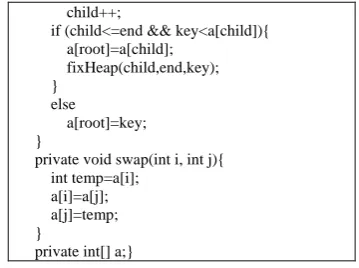
A. Heap:

This algorithm works with a complete binary tree (each node has only two children) and coping with the following three specific order properties: (A) All descendant nodes of a given node N are less or equal than the content of N; (B) All ancestors of N are greater or equal than the contents of N; (C) Consequently, all nodes are smaller than the root of the binary tree. An appealing feature of this methodology relies in its vector representation: the children of node i are located in position (2i) and (2i+1) whilst the father of the same node i is at position ((int) i/2).

Table III. Main Java code of Heap sort by Mohr (www.augustana.ab.ca/~jmohr/courses /2004.winter/csc310/source/HeapSort.java.htm).

public class HeapSort{

public HeapSort(int[] anArray){ a=anArray;}

public void sort(){ sort(a.length-1);} public void sort(int end){ for (int i=end/2;i>=0;i--) fixHeap(i,end,a[i]); for (int i=end;i>0;i-- ){ swap(0,i);

fixHeap(0,i-1,a[0]);} }

private void fixHeap(int root,int end, int key){ int child=2root;

if (child<end && a[child]<a[child+1])

child++;

if (child<=end && key<a[child]){ a[root]=a[child];

fixHeap(child,end,key); }

else

a[root]=key; }

private void swap(int i, int j){ int temp=a[i];

a[i]=a[j]; a[j]=temp; }

private int[] a;}

B. Insertion:

This methodology involves a sequential vector element-by-element scanning, moving it and placing it in any position whenever need it. Every insertion removes an element from the input data, inserting it into the correct position in the already sorted list, until no input elements remain. As expected, the choice of which element to remove from the input is arbitrary.

Table IV. Main Java code of Insertion sort (faculty.kfupm.edu.sa/ics/lahouari/Teaching/Sorting-1.ppt)

public class InsertionSort {

public InsertionSort(int[] anArray){ a=anArray;}

public void sort(){

for (int i=1;i<a.length;i++){ int next=a[i];

int j=i;

while (j>0 && a[j-1]>next){ a[j]=a[j-1];

j--; } a[j] = next;

for (int i=1;i<a.length;i++){ int j;

int next=a[i];

for (j=i-1; (j>=0) && (a[j]<next);j--){ a[j+1]=a[j];}

a[j+1]=next;} }

private int[] a;}

C. Bubble:

Also known as the sinking sort, it is a plain algorithm that works by repeatedly stepping through the list to be sorted, comparing each pair of adjacent items and swapping them if they are in the wrong order. This heavy overstep through the whole list is repeated until no swaps are needed, which suggests that the list is already sorted.

Table V. Main Java code of Bubble sort (mathbits.com/mathbits/Java/arrays/Bubble.htm).

public class BubbleSort{

public BubbleSort(int[] anArray){ a=anArray; }

public void sort() { int i,j,t=0;

for(i=0;i<a.length;i++){ for(j=1;<(a.length-i); j++){ if(a[j-1]>a[j]){ t=a[j-1]; a[j-1]=a[j]; a[j]=t;} }

t=a[j]; a[j]=a[j+1]; a[j+1]=t;} }

} }

private int[] a; }

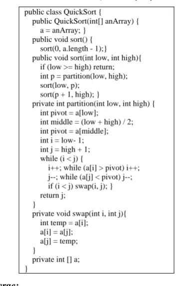
D. Quick:

Given a vector of elements, T[n], this algorithm choose arbitrarily a pivot x such that all elements smaller than x are on the left side of the vector while the remaining ones are on the right side. Typically, this pivot is usually the median or the average number of elements in order to achieve a balanced performance.In computer terms, this process goes through the following operations: (A) Walking the vector T from the left until T[i]>=x; (B) Walking the vector from the right until T[j]<=x; (C) Replace T[i] with T[j]; (D) Continue this process until i and j indices intersect.

Once again, the vector T[Left…Right] is divided such that: (A) The values T[Left], T[Left+1],...,T[j] are less than or equal x; (B) The values T[i], T[i+1],...,T[Right] is greater than or equal to x (with i=j+1). By using the divide and conquer strategy, the available vector, T[n]=T[Left…Right], will be split in two ones such that T[n]=T[Left...Right]=T[Left…j] +T[i…Right].When the cardinality of the domain [Left...j] is zero or one, then the first condition is accomplished.Similarly, when T[i...Right] becomes zero or one, the second condition is verified, meaning that this branch of the vector has been sorted.

Table VI. Main Java code of Quick sort by Cay Horstmann.

public class QuickSort {

public QuickSort(int[] anArray) { a = anArray; }

public void sort() { sort(0, a.length - 1);}

public void sort(int low, int high){ if (low >= high) return; int p = partition(low, high); sort(low, p);

sort(p + 1, high); }

private int partition(int low, int high) { int pivot = a[low];

int middle = (low + high) / 2; int pivot = a[middle]; int i = low- 1; int j = high + 1; while (i < j) {

i++; while (a[i] > pivot) i++; j--; while (a[j] < pivot) j--; if (i < j) swap(i, j); } return j;

}

private void swap(int i, int j){ int temp = a[i];

a[i] = a[j]; a[j] = temp; }

private int [] a; }

E. Merge:

Conceptually, the merge sort works as follows: If the present list is of length 0 or 1, then it is already sorted. Otherwise, divide the unsorted list into two sub-lists of about half of its size and sort each sub-list recursively by re-applying

the merge sort. At last, merge the two sub-lists back into one sorted vector.

Table VII. Main Java code of Merge sort (faculty.kfupm.edu.sa/ics/lahouari/Teaching/Sorting-2.ppt).

public class MergeSort {

public MergeSort(int[] anArray) { a= anArray;}

public void sort() { if (a.length<=1) return; int[] first=new int[a.length / 2];

int[] second=new int[a.length-first.length]; System.arraycopy(a, 0, first, 0, first.length); System.arraycopy(a, first.length, second, 0, second.length);

MergeSort firstSorter = new MergeSort(first); MergeSort secondSorter = new MergeSort(second); firstSorter.sort();

secondSorter.sort(); merge(first, second); }

private void merge(int[] first, int[] second){ int iFirst=0;

int iSecond=0; int j=0;

while (iFirst<first.length && iSecond <second.length) { if (first[iFirst]>second[iSecond]){

a[j]=first[iFirst]; iFirst++;} else {

a[j]=second[iSecond]; iSecond++;} j++;}

System.arraycopy(first, iFirst, a, j, first.length- iFirst);

System.arraycopy(second, iSecond, a, j, second.length - iSecond);} private int[] a;

}

III. COMPARATIVEANALYSIS

The present procedure will consider the response time of the sort methodology in question as the critical factor. As the records number to sort within the vector plays a major component in this benchmark, theoretically, the relevant complexity measured by the different schemes are the number of comparisons between keys, C(n), and the number of movements of items within the vector, M(n). Clearly, the economic use of RAM memory is also a primary requirement regarding internal ordering.

Table VIII. Elapsed consuming time of each sort method per OS and array size in a tabular context.

Windows 7 Linux Ubuntu

Merge Sort

Array Size(n) Elapsed Time (milliseconds)

Elapsed Time (milliseconds)

10000 0 63

100000 46 115

1000000 390 370

10000000 3806 3492

20000000 ₄₉₆₈₇ 6779

Insertion Sort

Array Size(n) Elapsed Time (milliseconds)

Elapsed Time (milliseconds)

10000 125 77

100000 14133 7047

1000000 1970165 1220783

10000000 213086732 181750608

20000000 - -

Bubble Sort

Array Size(n) Elapsed Time (milliseconds)

Elapsed Time (milliseconds)

10000 281 219

100000 33977 24143

1000000 3682330 2705360

10000000 357617355 276336651

20000000 - -

Quick Sort

Array Size(n) Elapsed Time (milliseconds)

Elapsed Time (milliseconds)

10000 0 35

100000 15 46

1000000 93 170

10000000 874 876

20000000 1809 1748

Heap Sort

Array Size(n) Elapsed Time (milliseconds)

Elapsed Time (milliseconds)

10000 0 36

100000 31 59

1000000 281 347

10000000 3369 3765

20000000 7036 7870

Some comments can be drawn by table eight and nine: a. The time sorting resolution is lower for the Ubuntu®

environment when Insertion and Bubble is applied (the speed ratio between Windows® and Linux® varies between 0.5 and 0.8). However, Windows® 7 performs best with

Merge, Quick (the speed ratio decreases from 1.9 to 1.1) and Heap, particularly with low vector sizes.

b. With Insertion and Bubble methods, the response time difference between Ubuntu® and Seven® increases directly with the amount of input considered. With Merge and Heap, this pattern can also be found for Seven®.

c. Inexplicably, Quick reveals a strange behavior, that is, until ten million records, Windows® presents lower sorting times but when the number of records doubles to twenty million, Linux® beats Windows® clearly, (the speed ratio decreases from 3 to 0.96). This outlier situation can also be verified with Merge sort (the same speed ratio decreases from 2.5 to 0.13).

d. By exploring the next ten images of table nine, there is a general drift for a positive linear response time for all algorithms. Yet, this response time grows exponentially when the input size vector increases from 10 million to 20 million.

e. Whether the OS considered, Quick and Bubble are the fastest and slowest sort algorithm, respectively.

Table IX. Elapsed consuming time of each sort method per OS and the lowest array size (in order to highlight the differences due to the global scale

is quite wide) in a graphical context.

Merge Sort

Insertion Sort

Bubble Sort

Quick Sort

IV. CONCLUSION

With this practical assessment on the performance of sorting algorithms but closely dependent on the OS and its Java compiler, this article does not aim to address which OS performs best. Although they are direct competitors, both OS have their own history and context. This evaluation is just

another benchmark analysis to be added to other tests already performed by other companies and individuals. Whatever it is the case, the present authors guarantee the impartiality and the honesty factors of the present outcomes. Fundamentally, this research clearly suggests that the same Java code becomes faster both on Linux and on Windows with different sort methods. Concerning the reason of this dual behavior is a question that remains open to experts from other subjects such as compilers or operating systems. Collaterally, with the array size of 20 million cells, Bubble and Insertion did not achieve the initial ascending sort goal in a reasonable response time.

V. ACKNOWLEDGMENT

The present authors would like to offer our sincerest gratitude to FDCT (The Science and Technology Development Fund) of Macao, China, for supporting this research through the project number 060/2010/A.

VI. REFERENCES

[1] Garey, M, Johnson, D (1979). Computers and Intractability A Guide to the Theory of NP-Completeness. Freeman Press. [2] Ling, L (2006). Data complexity in machine learning and novel

classification algorithms. PhD Thesis, California Institute of Technology. CaltechETD etd-04122006-114210.

[3] Mohan, C (2008). Design and Analysis of Algorithms. ISBN 978-81-203-3517-2, Prentice Hall.