3473
Quantitative Analysis of Prewitt Edge Detector for
Brain Tissue Segmentation in Single-Channel MR
Image
Ghanshyam D. Parmar
1, Heena B. Sorathiya
2,
Department of Biomedical Engineering1,2,GEC GAndhinagar1,2Abstract-Segmentation of brain tissues is one important process prior to many analysis and visualization tasks for Magnetic Resonance (MR) images. Edge is one of the important characteristic features used in many image segmentation techniques for brain tissue segmentation in MR image. Prewitt approximation is technique used for detection of edges in any image. Unfortunately, MR images always contain significant amount of noise caused by operator performance, equipment and the environment. This noise can lead to major inaccuracies in edge detection process and hence in segmentation result. We conduct the research in measuring the performance of Prewitt approximation for edge detection in different noise level for single-channel MR image. To validate the accuracy and robustness of Prewitt approximation we carried out experiments on simulated MR brain scans. The performance of edge detector is analyzed by different quantitative measures. These quantitative measures include the mathematical measures like mean square error, signal to noise ratio and peak signal to noise ratio as well the statistical measures like accuracy, sensitivity, specificity and F measure
Index Terms-Brain tissue classification, Edge detection, F measure Magnetic Resonance, MR Images, Prewitt approximation, Segmentation, Sensitivity, Specificity
1. THE MAIN TEXT
Magnetic resonance imaging (MRI) or nuclear magnetic resonance imaging (NMRI) [1], [2] is primarily medical imaging technique used in radiology to visualize internal structure of the body. MRI provides much greater contrast among different soft tissues of body. This ability makes it useful for neurological, musculoskeletal, cardiovascular and oncological imaging [3]. Brain matter could be generally categorized as White Matter (WM), Gray Matter (GM) and Cerebrospinal Fluid (CSF) [4], [5]. Most of brain structures are anatomically defined by the boundaries of these tissue classes [4]–[6]. So, we need a method of segmenting tissues in classes. It is an important step for quantitative analysis of the brain and its anatomical structures. Brain tissue classification is also an important step for detection of various pathological conditions affecting brains parenchyma [7]–[9]. It is also used for surgical planning and simulation [10] and three-dimensional visualization for diagnosis and detection of abnormalities [11]–[13]. It is also useful in the study of brain development [13]–[15] and human aging [15], [16].
In MR imaging, images are produced based on intensities achieved by three tissue characteristics namely: T1 relaxation time, T2 relaxation time and proton density (PD). The images obtained by these properties are known as T1- weighted MR images, T2-weighted MR images and proton density MR images respectively. The effect of these parameters image can be varied based on the adjusting the parameters like
time to echo (TE) and time to repeat of the pulse sequence [17]. By using different parameters or number of echoes in the pulse sequence, a multitude of nearly registered images with different characteristics of same object can be achieved. If only a single MR image of the object is available such an image is referred to as single-channel (single-echo) image, and in case when number of MR images of the same object at same section are obtained, they are referred as multi-channel (multispectral or multi-echo) images [18]. For a given scanning time, the voxel sizes achieved in multi-spectral images are larger than those achieved with single-channel images. This ability of finer voxel sizes makes single-channel image more suitable for precise and accurate quantitative measurements of anatomical structures and tissues. Nevertheless, multichannel image provides more information at given voxel size than single-channel image[17], [18]. Most of segmentation techniques have relied on multi-spectral characteristics of MR images while a few studies have reported segmentation form single-channel MR images [19]. Here we explore the segmentation using single-channel MR images.
3474 surface and texture also result in the edge. The
non-geometrical events like shadows, secularities and internal reflection also result in edge in the image. The separation of different tissues and regions results as
edges in brain MR image result. Also, the abnormality within same tissue in brain MR image result in edge. Edge detection aim in identification of edges in the image by using different mathematical and statistical operations. This is achieved by detection of sharp discontinuity in the image intensity levels. The set of points at which this sharp discontinuity is observed results in curved or line segments known as edges. Edge detection is fundamental tool in different image processing, machine vision, image analysis, feature detection and feature extraction.
In section II, we present the Sobel–Feldman edge detector used for detection of edges in single-channel MR image used in this work. In section III, we present the result of the Prewitt edge detection approximation of single-channel MR image for different noise levels. Here we also present the quantitative analysis of the edge detection approximation with different statistical and mathematical measures. These quantitative measures include the mathematical measures like mean square error, signal to noise ratio and peak signal to noise ratio as well the statistical measures like accuracy, sensitivity, specificity and F measure. In section IV, the discussion of the results and the different quantitative measure is presented. Finally, the research work is concluded in section V.
2. PREWITT EDGE DETECTOR
Prewitt edge detector approximation was proposed by J.M.S.Prewitt presented the idea of an 3x3 Image Gradient Operator in 1970. It is a discrete two-dimensional differential operator used to emphasize and detect the gradient of the intensity function of image. The result of this operator corresponds either to the intensity gradient or the norm of the intensity gradient in the image. This is based on convolution of the image with two separable and integer valued horizontal and vertical operators, frequently known as masks. Given the input image I(x,y) of size m by n, where x=1,2…,n and y=1,2,…,n are horizontal and vertical indices of the image [20]–[24].
[
] and [
]
Where PFx and PFy are derivative approximation in
horizontal and vertical direction respectively. They are separable and integer valued small filters in horizontal and vertical directions. By convolving the I(x,y) with
Noise
Original MR
Image
Prewitt Edge
Approximation
0
1
3
5
7
[image:2.595.70.292.99.694.2]9
Table 1 Original MR Image, Prewitt Edge
approximation with respective Noise Level in
3475 Gx and Gy we obtain two different images with
horizontal and vertical edge approximation
( ) ( )
Where * is the convolution operator and Gx and Gy are
the horizontal and vertical edge approximations respectively. The final edge image is obtained by computing the gradient approximation with equation:
( ) √
The resulting image E(x,y) is known as Prewitt Edge approximation of original image I(x,y). Due to the separable, integer valued and small size nature of this edge detection approximation, it is relatively inexpensive in computations. Also it produces significant behavior in the high frequency and sharp discontinuity intensity variation in the image. Although the formulation of Prewitt edge detector approximation generally used form two dimensional images, this edge detector approximation can be further extended to other higher dimensions in case we have the higher dimensional image for the purpose of multi-dimensional edge detection [12], [20], [29], [21]–[28].
3. RESULTS
As the interest in computer-aided, quantitative analysis of medical image data is growing, the need for validation of such techniques is also increased. For the solution of validation problem, Simulated Brain Database (SDB) is available [30]. The Simulated Brain Database contains a set of realistic MRI data volumes [31] produced by a MRI simulator [32]. This data set is used in our work to evaluate the performance of the tissue classification algorithms in a setting where the truth is known [33]. The detail about the noise used in our work for analysis is described in [30]–[33]. Table 1 represents the Original MR Image, Prewitt Edge approximation with respective Noise Level in Percentage. Here, first column represents different noise levels in the percentage, the second column represents the single-channel MR image with the respective noise level from column 1. The third column represents the Prewitt Edge approximation for the MR image in the second column.
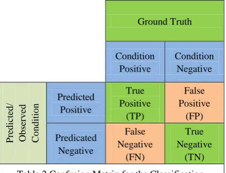
After obtaining the confusion matrix for any classification experiment result we have the True Positive (TP), True Negative (TN), False Positive (FP) and False Negative (FN), which are the number of counts in respective class. The confusion matrix for the classification Problem is shown in Table 2.
Ground Truth Condition Positive Condition Negative Pre d icted / Ob ser v ed C o n d itio
n Predicted Positive
[image:3.595.304.534.203.379.2]True Positive (TP) False Positive (FP) Predicated Negative False Negative (FN) True Negative (TN) Table 2 Confusion Matrix for the Classification
The Accuracy is defined as
The F Measure is defined as
The Mean Square Error (MSE) is defined as
‖ ‖
The Signal to Noise Ratio (SNR) is defined as
(
)
The Peak Signal to Noise Ratio (SNR) is defined as
(
√
)
The L2 Norm Ratio is defined as
‖ ‖
3476 Above mentioned measures are computed for the
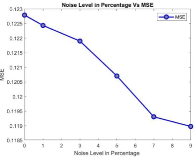
[image:4.595.311.509.102.262.2]single-channel MR images and respective Prewitt edge detector approximations in Table 1. The noise Vs measures are potted in the following figures.
[image:4.595.74.276.191.353.2]Figure 1 Noise Level in Percentage Vs Accuracy for the Prewitt Edge approximation
[image:4.595.315.509.313.473.2]Figure 2 Noise Level in Percentage Vs Specificity for the Prewitt Edge approximation
Figure 3 Noise Level in Percentage Vs Sensitivity for the Prewitt Edge approximation
Figure 4 Noise Level in Percentage Vs F measure for the Prewitt Edge approximation
[image:4.595.76.276.397.560.2] [image:4.595.310.509.522.683.2]3477
[image:5.595.80.276.286.449.2]Figure 6 Noise Level in Percentage Vs SNR for the Prewitt Edge approximation
Figure 7 Noise Level in Percentage Vs PSNR for the Prewitt Edge approximation
Figure 8 Noise Level in Percentage Vs L2 Norm Ratio for the Prewitt Edge approximation
Figure 1 represents the noise level in percentage vs accuracy for the Prewitt edge approximation. Figure 2 represents the noise level in percentage vs specificity for the Prewitt edge approximation. Figure 3
represents the noise level in percentage vs sensitivity for the Prewitt edge approximation. Figure 4 represents the noise level in percentage vs F measure for the Prewitt edge approximation. Figure 5 represents the noise level in percentage vs MSE for the Prewitt edge approximation. Figure 6 represents noise level in percentage vs SNR for the Prewitt edge approximation. Figure 7 represents the noise level in percentage vs PSNR for the Prewitt edge approximation. Figure 8 represents the noise level in percentage vs L2 norm ratio for the Prewitt edge approximation. The exploration of these results is discussed in the section IV.
4. DISCUSSION
The Sibel-Feldman edge detection approximation detects the edges in single-channel MR image in different noise levels. As the noise level increases the detected edges are not continuous line segments instead they are isolated small pixel group appearing as small edge like structures. These small structures are appearing high number as the noise level increases. This small edge like structures causes most of quantitative measures mislead toward results. Due to these, the accuracy of the Prewitt approximation increases as the noise level in the single-channel MR image increases. The specificity of the Prewitt approximation decreases as the noise level in the single-channel MR image increases. The sensitivity of the Prewitt approximation increases as the noise level in the single-channel MR image increases. The F measure value of the Prewitt approximation increases as the noise level in the single-channel MR image increases. The MSE of the Prewitt approximation decreases as the noise level in the single-channel MR image increases. The SNR of the Prewitt approximation increases as the noise level in the single-channel MR image increases. The PSNR value of the Prewitt approximation increases as the noise level in the single-channel MR image increases. The L2 Norm Ratio of the Prewitt approximation decreases as the noise level in the single-channel MR image
increases
□
5. CONCLUSION
[image:5.595.85.275.495.658.2]3478 include the mathematical measures like mean square
error, signal to noise ratio and peak signal to noise ratio as well the statistical measures like accuracy, sensitivity, specificity and F measure. The proper selection of measure can give comparative results for detection of edge approximation in single-channel MR image for tissue segmentation.
REFERENCES
[1] P. C. Lauterbur, “Image Formation by Induced Local Interactions: Examples Employing Nuclear Magnetic Resonance,” Nature, vol. 242, no. 5394, pp. 190–191, Mar. 1973. [2] P. C. Lauterbur, “Magnetic resonance
zeugmatography,” Pure Appl. Chem., vol. 40, no. 1–2, pp. 149–157, 1974.
[3] L. F. Squire, Fundamentals of radiology, 4th ed. Harvard University Press, 1988.
[4] H. Damasio, Human brain anatomy in computerized images, 2nd ed. Oxford University Press US, 2005.
[5] P. B. Henri M. Duvernoy, The human brain: surface, three-dimensional sectional anatomy with MRI, and blood supply, 2nd ed. Springer, 1999.
[6] J. Nolte, The human brain: an introduction to its functional anatomy. Mosby, 1981.
[7] C.R.Jack, “Brain and cerebrospinal fluid volume: Measurement with MR imaging,”
Radiol., vol. 178), pp. 22–24, 1991.
[8] T. E. Schlaepfer, G. J. Harris, A. Y. Tien, L. W. Peng, S. Lee, E. B. Federman, G. A. Chase, P. E. Barta, and G. D. Pearlson, “Decreased regional cortical gray matter volume in schizophrenia,” Am. J. Psychiatry, vol. 151, no. 6, pp. 842–848, 1994.
[9] O. W.L., L. F.M., D. M. Mills, and D. Norman, “White matter disease in Aids: Finding at MR imaging,” Neuroradiol, vol. 169, pp. 445–448, 1988.
[10] K. Fitzgerald, “Medical electronics,” IEEE Spectr., vol. 28, no. 1, pp. 76–78, 1991. [11] R. R.A, Three-Dimensional Biomedical
Imaging. New York: VCH, 1995.
[12] M. E. Brummer, M. R.M., R. L. Eisner, and R. R. J. Lewine, “Automatic detection of brain contours in MRI data sets,” IEEE Trans. Med. Imag., vol. 12, no. 2, pp. 153–166, 1993. [13] A. K. H. Miller, R. L. Alston, and J. A. N.
Corsellis, “Variation with age in the volumes of gray and white matter in the cerebral hemispheres of man: Measurement with an image analyzer,” Neuropathol., Appl. Neurobiol., vol. 6, pp. 119–132, 1980.
[14] A. T., R. R., S. L. Vanhanen, M. Kallio, and Santavuori, “MRI of normal brain from early childhood to middle age,” Neuroradiol, vol. 36, pp. 644–648, 1994.
[15] D. G. M. Murphy, C. DeCarli, M. B. Schapiro, S. I. Rapoport, and B. Horwitz, “Age-related differences in volumes of subcortical nuclei, brain matter, and cerebrospinal fluid in healthy men as measured with magnetic resonance imaging,” Arch. Neurol., vol. 49, pp. 839–845, 1992.
[16] K. O. Lim, R. B. Zipursky, M. C. Watts, and A. Pfefferbaum, “Decreased gray matter in normal aging: An in vivo magnetic resonance study,” J. Gerontol. Biol. Sci., vol. 47, no. 1, pp. B26-30, 1992.
[17] R. H. Hashemi, W. G. Bradley, and C. J. Lisanti, MRI: the basics, 2nd ed. Lippincott Williams & Wilkins, 2004.
[18] D. W. McRobbie, E. A. Moore, and M. J. Graves, MRI from picture to proton. Cambridge University Press, 2003.
[19] J. C. Rajapakse, J. N. Giedd, and J. L. Rapoport, “Statistical approach to segmentation of single-channel cerebral MR images,” IEEE Trans. Med. Imaging, vol. 16, no. 2, pp. 176–186, 1997.
[20] J. M. Prewitt, “Object ENhancement and Extraction,” Picture Processing and Psychopictorics,Academic Press. New York, 1970.
[21] J. Kittler, “On the accuracy of the Sobel edge detector,” Image Vis. Comput., vol. 1, no. 1, pp. 37–42, 1983.
[22] A. K. Jain, Fundamentals of digital image processing. Englewood Cliffs, NJ: Prentice Hall, 1989.
[23] W. K. Pratt, Digital image processing: PIKS Scientific inside, vol. 4. Wiley-interscience Hoboken, New Jersey, 2007.
[24] I. Pitas and A. N. Venetsanopoulos, “Order statistics in digital image processing,” Proc. IEEE, vol. 80, no. 12, pp. 1893–1921, 1992. [25] Z. Jin-Yu, C. Yan, and H. Xian-Xiang, “Edge
detection of images based on improved Sobel operator and genetic algorithms,” in Image Analysis and Signal Processing, 2009. IASP 2009. International Conference on, 2009, pp. 31–35.
[26] H. Tang, E. X. Wu, Q. Y. Ma, D. Gallagher, G. M. Perera, and T. Zhuang, “MRI brain image segmentation by multi-resolution edge detection and region selection,” Comput. Med. Imaging Graph., vol. 24, no. 6, pp. 349–357, 2000.
[27] M. S. Atkins and B. T. Mackiewich, “Fully automatic segmentation of the brain in MRI,”
IEEE Trans. Med. Imaging, vol. 17, no. 1, pp. 98–107, 1998.
3479
Image Anal., vol. 1, no. 2, pp. 109–127, 1996. [29] I. Pitas, Digital image processing algorithms
and applications. John Wiley & Sons, 2000. [30] C. A. Cocosco, V. Kollokian, R. K.-S. Kwan,
G. B. Pike, and A. C. Evans, “BrainWeb: Online Interface to a 3D MRI Simulated Brain Database,” Neuroimage, vol. 5, p. 425, 1997. [31] R. K. Kwan, A. C. Evans, and G. B. Pike,
“MRI simulation-based evaluation of image-processing and classification methods.,” IEEE Trans Med Imaging, vol. 18, no. 11, pp. 1085– 1097, Nov. 1999.
[32] R. Kwan, A. C. Evans, and G. B. Pike, “An Extensible MRI Simulator for Post-Processing Evaluation,” in Springer-Verlag, 1996, pp. 135–140.