Division V
SDOF Response to Pump Start Loading
Matthew Cepkauskas1
, Juyoung Kim2
1 Senior Engineer, GE Oil & Gas, Jacksonville, FL 32221, USA 2. Engineer, GE Oil & Gas, Jacksonville, FL 32221, USA
Abstract
The present paper investigates the response of a simple Single Degree of Freedom (SDOF) spring mass model subjected to a force caused by an acoustic pressure wave during pump start. This simple model provides the mathematical preliminaries to solve the more complex problem of the coupled acoustic/structure interaction with acoustic amplification that will be performed in a subsequent paper. This exercise is intended to help resolve the question; how fast does a pump need to go through a structural resonance and not have significant response? The solution is obtained using Duhamel integral with a pump having an output amplitude and a driving frequency that is a function of time. The resulting closed form solutions for three cases are provided and investigated numerically. The result is compared with existing literature.
INTRODUCTION
The subject of vibrations starts with the simple single degree of freedom spring mass model (SDOF). This simple model can be used to understand many real physical vibration systems. It is also the underlying time dependency of beam, plate, shell and finite element models along with the bases for many other engineering and physics theory.
) (t f kx x c x
m (1)
where,
m = mass associated with the structural system
x= acceleration of the system (second derivative of displacement with respect to time)
c = damping of the structural system
x = velocity of the system (first derivative of displacement with respect to time)
k = stiffness of the structural system x = displacement of the system f(t) = Generic applied force
An examination of a simple acoustic/structural model can be found in Cepkauskas & Stevens (1981)
where the pump operated at steady state conditions with a pump exit pressure
P
0cos
pt
, where P0 isthe amplitude of the pressure wave with harmonic pump frequency ωp. The problem of interest in this
paper is for start-up conditions where it is expected that the pressure wave is generated by a source of the
form,
at
sin(
bt
2
.
0t
)
with the amplitude aP0psi at the time the pump reaches its steady statecondition (i.e. time for the pump to come to full speed,); .0
is an initial steady state frequency.
Thevalue of the constant
p
b is found when the rotational speed reaches steady state conditions. See
MATHEMATICAL FORMULATION
Three cases will be considered:
1. Constant amplitude but changing driving frequency asin(bt2.0t)
2. Case 1 with damping
3. Case 1 with changing amplitude and driving frequency
The response for all three cases is determined using the Duhamel Equation used in Cepkauskas & Stevens, but for simplicity applies the load directly to the SDOF. Later the more complex fluid structure interaction will be examined where these same integrals are required.
Case 1 can be re-written as:
) ( )
( )
( 2 P t
M A t x t
x (2)
with 2
is used to represent the structural natural frequency with M being the structural mass and A is
area of the structure upon which the pressure acts.
The solution to this differential equation can be obtained by the well-known Duhamel integral:
P t d
M A t
x() 0t ( )sin ( ) (3)
The integration is a formidable task for a forcing function of ( ) sin( 2 0 )
t bt a t
P . This forcing function
is constant in amplitude and the time dependent rotational speed is changing with time. where 0is added
to simulate a variable speed pump operating at a particular rpm and then is ramped to a higher or lower
rpm. This makes the integral more manageable. Substitution of () sin( 20)
b a
P into equation 3
and expanding both sin terms in terms of their complex exponential identity results in:
)*sin[ ( )]
sin( 2 0
t
b
4 4
4 4
0 2 0
2 0
2 0
2 ( ) ( ) ( )
)
(t i bi i t i bi i t i bi i t i bi i
e e e
e e e
e e e
e e
e
Consider, for example the first term, it can be re-written as:
4 ) (2 0
i t ei b
e . The goal is to make the second exponential a perfect square. This is accomplished
by multiplying by ei4be i4b
2 2
, which is equivalent to multiplying by one. Thus, the equation can be written as:
4 4
) ( 4
) 4 (
4
2 2
2
0 2
2
Z i t i b i b b
i t i b
i e
e e e
e
e
where
b b Z
2
2 0
Division V t T T FS T T FC T T FC T T FS b M A a t x 0 )} 4 sin( * ) 2 ( ) 4 cos( * ) 2 ( ) 3 cos( * ) 1 ( ) 3 sin( * ) 1 ( { 4 2 ) (
(4)
Only the upper integration limit, that is the particular solution, is of interest, where FS and FC are Fresnel sin and Fresnel cos integrals and the arguments are:
b bt T 2 ) 2 (
1 0 (5-a)
b bt T 2 ) 2 (
2 0 (5-b)
b t T 4 ) ( 3 2 0
(5-c)
b t T 4 ) ( 4 2 0
(5-d)
A solution to this problem for a=A=M==1.0 is given by Park, Do & Lopez (2011). The solutions are
identical when equations 4 and 5 are reduced with this condition.
Case 2 DAMPED CASE:
When damping, , is added to the Duhamel integral is given by:
P e t d
M A t
x t n
d ) ( sin ) ( )
( 0
, similar results is obtained
t A A A A A t x 0 5 4 3 2
1{ }
) (
Re (6)
with the natural frequency replaced by the damped natural frequency, 2
2
2 1
d , again the upper limit containing the particular solution is of interest and the required
terms modified to include damping as follows:
4 4 ) 2 4 2 4 ( 1 1 8 2 0 2 0 0 2 2 b M e A A d b i i i t ib b
i n n n n d d d d
(7-a) ] 2 ) ) 2 ( ( 1 [ 0 4 2 2 2 2 b i bt i erf e
A b d
i n
(7-b)
] 2 ) ) 2 ( ( 1 [ 0 4 2 ) 2 4 ( 3 2 0 2 0 b i bt i i erf ie
A b d
t b
i d d d
(7-c) ] 2 ) ) 2 ( ( 1 [ 0 4 2 2 4 2 4 0 2 2 b i bt i erf e
A b d
i ib
i n d n d d
(7-d) ] 2 ) ) 2 ( ( 1 [ 0 4 2 2 5 2 0 2 b i bt i i erf ie
A b d
i i d d n
(7-e)
Case 3 Changing amplitude and driving frequency
t
B B B b
b M
A a t x
0 3 2 1 2 5
2 3 2
5 4 }
2 { 2 )
(
(8)
] )
( sin[ ] )
(
sin[ 2 0
0 2
1 bx x t bx x t
B n n n n
(9-a)
)] 2 ( ) 4 cos( ) 2 ( ) 4 )[sin(
( 0
2 T S T T C T
B n
(9-b)
)] 1 ( ) 3 cos( ) 1 ( ) 3 )[(sin(
( 0
3 T S T T C T
B n
(9-c)
NUMERICAL RESULTS
Note the plots that follow use the particular solution designations of xp(t) for case 1, xnew_p(t) for
case 2 and xxp(t) for case 3.
Figure 1 shows a change in both pump amplitude and frequency. Note that this is made up of
both case 1 and case 3 forcing function to meet the interface conditions at t=1.0 & t=2.0 s, that is
the interface equation is
( ) ( )sin( 2 0 )t bt Bt A t
P
, with
A(2P0P1)and
B(P1P0), where
P0 and P1 are the steady state pressure amplitude from t=0 to t=1 second and t=2 seconds to t=3
seconds, respectively, with corresponding 20 HZ and 30 HZ pump speed.
0 1 2 3
2
1
0 1 2
FIGURE 1 PUMP PRESSURE CHANGE FROM 20 HZ with AMP 0.5 psi TO 30 HZ & 2.0 psi
P t( ) psi
t
Park (2011) identifies a unique jump phenomenon for case 1 where resonance occurs prior to the expected resonance at the spring mass natural frequency. This is shown in Figure 2 with parameters a=1.0 psi, A=100inch^2 and M=1E6 lb where the jump frequency is (3 Hz-0 Hz)/2 = 1.5 Hz where a response increase exists at 1.5 Hz for a ramp rate of 1E-2 rad/sec^2.
1 2 3 4 5
0.01
5
103 0 5 10 3
0.01
Figure 2: CASE 1 - w0=0, wn=3, b=1x10^-2
Displacement
xp t()
Division V
Figure 3 shows the comparison of case 1 with case two with a very small damping value of 1E-10. Similar results are obtained.
A
0 1 2 3 4
4
103 2
103 0 2 10 3
4 10 3
Figure 3: Case 1 compared to Case 2 with zeta=1x10⁻¹⁰ Rex new_p ( )t
x p t( )
b t0
A more realistic value of damping of 1E-03 is shown in Figure 4.
0 1 2 3 4
4
103
2
103
0 2 10 3
4 10 3
Figure 4: Case 1 compared to Case 2 with zeta=1x10⁻³
Re xnew_p t ( ) xp t( )
b t0
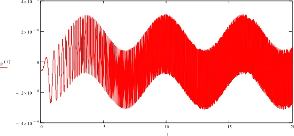
For case 3, different parameters are used to identify a more interesting case where a local and global oscillation occur with a frequency 1/12.5 sec = 0.8 Hz which is the jump frequency = (1.0 Hz-0.6 Hz)/2. This case needs added scrutiny along with a damped solution in the future.
0 5 10 15 20
4
106 2
106 0 2 10 6
4 10 6
Figure 5: Case 3 with w0=0.6 and wn=1.0
xx p t( )
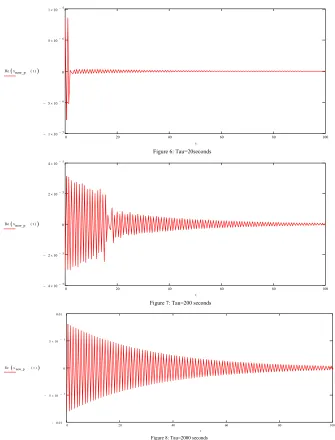
The next three figures examine the magnitude and number of oscillations for a more realistic case of a pump speed, that starts at zero Hz and climbs to 20 Hz over various times that the pump reaches its full speed with a natural frequency of 5 Hz. Figure 6 is for a very quick pump start of 20 seconds with a ramp rate of b=9.4 rad/sec^2, figure 7 with a pump start time of 200 seconds and ramp rate of 0.94 rad/sec^2 and figure 8 with a very long pump start of 2,000 seconds and a ramp rate of 0.094 rad/sec^2. The amplitude increases with smaller ramp rates and the number of oscillations increase.
0 20 40 60 80 100
1
105
5
106 0 5 10 6
1 10 5
Figure 6: Tau=20seconds
Re x new_p ( )t
t
0 20 40 60 80 100
4
105 2
105 0 2 10 5
4 10 5
Figure 7: Tau=200 seconds
Re x new_p ( )t
t
0 20 40 60 80 100
0.01
5
103 0 5103 0.01
Figure 8: Tau=2000 seconds
Rex new_p ( )t
Division V
CONCLUSIONS
Three cases of transient pump start have been considered. Numerical results show that the amplitude and number of cycles increases as the ramp rate slows down. This agrees with Park (2011) that identifies the jump phenomenon based on numerical integration. Additional information can be found in the Park paper by replacing the ramp rate based on a natural frequency of 1 Hz, with the present ramp rate in the form of
2 1
d
b
. Further investigation of case 3 with damping needs to be considered. The Integrals
presented in this paper could now be used to solve the more complex problem of
acoustic/structure interaction found in Cepkauskas (1983).
REFERENCES
Cepkauskas, M.M. & Stevens, J.A., “Fluid-Structure Interaction Via the Boundary Operator Method”, Journal of Sound and Vibrations, 1983, 90(2), pp. 229-236.